跳到论文正文
W Papers独立论文阅读器 arXiv:2304.13322 论文正文 计算阅读时间 · 0%
引用这篇论文根据当前论文元数据生成,正式投稿前建议核对。


License: CC BY 4.0
arXiv:2304.13322v1 [eess.SY] 26 Apr 2023

Event-triggered Boundary Control of a Class of Reaction-Diffusion PDEs with Time-dependent Reactivity

Bhathiya Rathnayake Affiliation: B. Rathnayake is with the Department of Electrical and Computer Engineering, University of California San Diego, La Jolla, CA 92093 brm222@ucsd.edu    Mamadou Diagne Affiliation: M. Diagne is with the Department of Mechanical and Aerospace Engineering, University of California San Diego, La Jolla, CA 92093 mdiagne@eng.ucsd.edu
Abstract

This paper presents an event-triggered boundary control strategy for a class of reaction-diffusion PDEs with time-varying reactivity under Robin actuation. The control approach consists of a backstepping full-state feedback boundary controller and a dynamic event-triggering condition, which determines the time instants when the control input needs to be updated. It is proved that under the proposed event-triggered boundary control approach, there is a uniform minimal dwell-time between two event times. Furthermore, the well-posedness and the global exponential convergence of the closed-loop system to zero in L2L^{2}-sense are established. A simulation is conducted to validate the theoretical developments.

I Introduction

Event-triggered control is a control technique which updates the control input only at events dictated by a suitable event generator [1] that utilizes current system states. This is in contrast to conventional sampled-data control [2, 3, 4] where the control input is updated at certain fixed times periodically or aperiodically irrespective of the system states. Thus, event-triggered control can be viewed as a sampled-data control approach that introduces feedback into communication and control update tasks. In event-triggered control, by exploiting the power of feedback, the control input is updated aperiodically only when needed, which significantly reduces the number of communications and control updates while maintaining a satisfactory closed-loop performance [5].

Typically, event-triggered control comprises two main components: a feedback control law that achieves the desired closed-loop performance and an event-triggered mechanism, which determines when to update the control input. A key requirement in event-triggered control is to rule out the so-called Zeno behavior, which is the occurrence of infinite number of control updates in a finite time interval. This is typically achieved via careful design of an event triggering mechanism for which there exists a guaranteed lower bound for the time between two successive events, known as the minimal dwell-time.

During the past years, various interesting results related to event-triggered control have been reported on systems described by both linear and nonlinear ordinary differential equations (ODEs) (see [1],[6]). This has kindled a vigorous interest in developing event-triggered control strategies for systems governed by partial differential equations (PDEs) [7, 8, 9, 10, 11, 12, 13, 14, 15, 16, 17]. In [7], an output feedback event-triggered boundary controller for 1-D linear hyperbolic systems of conservation laws is proposed using Lyapunov techniques. The authors of [8] design an observer-based event-triggered backstepping boundary controller for a coupled 2×22\times 2 hyperbolic system utilizing a dynamic triggering condition. Using ISS properties and small-gain arguments, the authors of [9] propose a full-state feedback event-triggered boundary control approach for constant parameter reaction-diffusion PDEs. In [12] and [13], event-triggered boundary control approaches for a class of constant parameter reaction-diffusion PDEs under anti-collocated and collocated boundary sensing and actuation are proposed using dynamic event-triggers. Recently, event-triggered boundary control strategies for the one-phase moving boundary Stefan problem have been proposed under both static [16] and dynamic [17] triggering conditions.

There are several recent works devoted to the study of boundary control of linear parabolic PDEs with nonconstant parameters [18, 19, 20, 21]. In [18], the authors propose backstepping boundary controllers for linear parabolic PDEs with space-dependent diffusivity or time-dependent reactivity. An exponentially stabilizing tracking controller based on backstepping and differential flatness methods is proposed in [19] for a linear parabolic PDE with spatially and temporally varying coefficients and nonlinear boundary input. The authors of [20] develop backstepping boundary controllers for coupled linear parabolic PDEs with space- and time-dependent coefficients. Deviating from [18, 19, 20], where one has to solve time varying gain kernel PDEs which capture space- and time-dependent coefficients, the authors of [21] propose to use a simpler kernel capturing only the spatial variation of the reaction coefficient. This is achieved by sampling the reaction term in time and regarding it constant between two successive sampling times which lead to a time-independent gain kernel PDE. In order to determine these sampling instants, the authors develop static and dynamic event-triggering mechanisms which ensure the global exponential stability of the closed-loop system under continuous-time backstepping boundary control. Despite the reaction term is sampled in time when obtaining the control gain, the control input still has to be continuously computed and applied to the plant. To the best of our knowledge, there are no prior works which address the event-triggered boundary control of infinite-dimensional systems with time-varying parameters.

In this paper, for the first time, we present an event-triggered boundary control of a class of reaction-diffusion PDEs with time-dependent reactivity under Robin actuation using infinite-dimensional backstepping approach. First we obtain a continuous-time boundary controller which we apply in a zero-order hold fashion between two sampling instants to obtain the event-triggered control input. We develop a dynamic event-triggering mechanism to determine the sampling instants when the control input needs to be computed and updated. Under the proposed event-triggering mechanism, we prove that the closed-loop system is Zeno-free. Furthermore, we establish the closed-loop system’s well-posedness and the global exponential convergence to zero in L2L^{2}-sense.

This paper is organized as follows. Section II introduces the class of linear reaction-diffusion system and the continuous-time event-triggered boundary control. Section III presents the event-triggered boundary control. A numerical exampled is provided in Section IV to illustrate the results, and the conclusion is provided in Section V.

Notation: ℝ+\mathbb{R}_{+} is the nonnegative real line whereas ℕ\mathbb{N} is the set of natural numbers including zero. By C0​(A,Ω)C^{0}(A;\Omega), the class of continuous functions on A⊆ℝnA\subseteq\mathbb{R}^{n} is denoted, which takes values in Ω⊆ℝ\Omega\subseteq\mathbb{R}. By Ck​(A,Ω)C^{k}(A;\Omega), where k≥1k\geq 1, the class of continuous functions on AA, which takes values in Ω\Omega and has continuous derivatives of order kk, is denoted. L2​(0,1)L^{2}(0,1) stands for the equivalence class of Lebesgue measurable functions f:[0,1]→ℝf:[0,1]\rightarrow\mathbb{R} such that ‖f‖=(∫01|f⁡(x)|2)1/2<∞\|f\|=\big(\int_{0}^{1}|f(x)|^{2}\big)^{1/2}<\infty. Let u:[0,1]×ℝ+→ℝu:[0,1]\times\mathbb{R}_{+}\rightarrow\mathbb{R} be given. u⁡[t]u[t] represents the profile of uu at certain t≥0t\geq 0, i.e., (u​[t])​(x)=u​(x,t),\big(u[t]\big)(x)=u(x,t), for all x∈[0,1]x\in[0,1]. For an interval J⊆ℝ+,J\subseteq\mathbb{R}_{+}, the space C0​(J,L2​(0,1))C^{0}\big(J;L^{2}(0,1)\big) is the space of continuous mappings J∋t→u⁡[t]∈L2​(0,1)J\ni t\rightarrow u[t]\in L^{2}(0,1).

II Continuous-time Backstepping Boundary Control

Let us consider the following scalar reaction-diffusion system:

ut​(x,t)\displaystyle u_{t}(x,t) =ε​ux​x​(x,t)+λ⁡(t)​u​(x,t),\displaystyle=\varepsilon u_{xx}(x,t)+\lambda(t)u(x,t), (1a)
ux​(0,t)\displaystyle u_{x}(0,t) =0,\displaystyle=0, (1b)
ux​(1,t)+q​u​(1,t)\displaystyle u_{x}(1,t)+qu(1,t) =U⁡(t),\displaystyle=U(t), (1c)

and the initial condition u⁡[0]∈L2​(0,1),u[0]\in L^{2}(0,1), where ε>0\varepsilon>0 is a constant, u:[0,1]×[0,∞)→ℝu:[0,1]\times[0,\infty)\rightarrow\mathbb{R} is the system state and U⁡(t)U(t) is the control input. The time-dependent reaction coefficient λ⁡(t)\lambda(t) satisfies the following assumption:

Assumption 1:

The reaction coefficient λ⁡(t)\lambda(t) satisfies

supt≥0|λ(n)​(t)|≤Dn+1​n!,\sup_{t\geq 0}|\lambda^{(n)}(t)|\leq D^{n+1}n!, (2)

for all t≥0,t\geq 0, where D>0D>0 is a constant.

Assumption 2:

The plant’s parameters qq and ε\varepsilon satisfy the following inequality

q>D+ε2​ε.q>\frac{D+\varepsilon}{2\varepsilon}. (3)
Remark 1:

Assumption 1 assumes λ⁡(t)\lambda(t) belongs to Gevrey class GM,R,α​(ℝ+)G_{M,R,\alpha}(\mathbb{R}_{+}) of order α=1\alpha=1 in ℝ+\mathbb{R}_{+} with M=DM=D and R=1/DR=1/D [19]. This makes λ⁡(t)\lambda(t) an analytic function of tt. Further, Assumption 1 is required to ensure the boundedness of the solution of the time-varying gain kernel and its certain spatial and time derivatives, which emanate from the backsteping (inverse) transform. Assumption 2 is required to avoid a trace term for which it is impossible to obtain a useful bound on its rate of change. In order to overcome this, it is required that q−D/2​εq-D/2\varepsilon is sufficiently large.

Proposition 1:

The invertible backstepping transformation

w⁡(x,t)=u⁡(x,t)−∫0xK⁡(x,y,t)​u​(y,t)​𝑑y,w(x,t)=u(x,t)-\int_{0}^{x}K(x,y,t)u(y,t)dy, (4)

where K⁡(x,y,t)K(x,y,t) satisfies

Kt​(x,y,t)=ε​Kx​x​(x,y,t)−ε​Ky​y​(x,y,t)−λ⁡(t)​K​(x,y,t),\displaystyle\begin{split}K_{t}(x,y,t)&=\varepsilon K_{xx}(x,y,t)-\varepsilon K_{yy}(x,y,t)\\ &\quad-\lambda(t)K(x,y,t),\end{split} (5a)
Ky​(x,0,t)\displaystyle K_{y}(x,0,t) =0,\displaystyle=0, (5b)
K⁡(x,x,t)\displaystyle K(x,x,t) =−λ⁡(t)2​ε​x,\displaystyle=-\frac{\lambda(t)}{2\varepsilon}x, (5c)

for 0≤y≤x≤1, and ​t≥0,0\leq y\leq x\leq 1,\text{ and }t\geq 0, and a control law U⁡(t)U(t) chosen as

U⁡(t)=∫01(r⁡(t)​K​(1,y,t)+Kx​(1,y,t))​u​(y,t)​𝑑y,U(t)=\int_{0}^{1}\Big(r(t)K(1,y,t)+K_{x}(1,y,t)\Big)u(y,t)dy, (6)

map the system (1) into the following target system:

wt​(x,t)\displaystyle w_{t}(x,t) =ε​wx​x​(x,t),\displaystyle=\varepsilon w_{xx}(x,t), (7a)
wx​(0,t)\displaystyle w_{x}(0,t) =0,\displaystyle=0, (7b)
wx​(1,t)\displaystyle w_{x}(1,t) =−r⁡(t)​w​(1,t),\displaystyle=-r(t)w(1,t), (7c)

where

r⁡(t)=q−λ⁡(t)2​ε.r(t)=q-\frac{\lambda(t)}{2\varepsilon}. (8)

The inverse transformation of (4) is given by

u⁡(x,t)=w⁡(x,t)+∫0xL⁡(x,y,t)​w​(y,t)​𝑑y,u(x,t)=w(x,t)+\int_{0}^{x}L(x,y,t)w(y,t)dy, (9)

where L⁡(x,y,t)L(x,y,t) satisfies

Lt​(x,y,t)=ε​Lx​x​(x,y,t)−ε​Ly​y​(x,y,t)+λ⁡(t)​L​(x,y,t),\displaystyle\begin{split}L_{t}(x,y,t)&=\varepsilon L_{xx}(x,y,t)-\varepsilon L_{yy}(x,y,t)\\ &\quad+\lambda(t)L(x,y,t),\end{split} (10a)
Ly​(x,0,t)\displaystyle L_{y}(x,0,t) =0,\displaystyle=0, (10b)
L⁡(x,x,t)\displaystyle L(x,x,t) =−λ⁡(t)2​ε​x,\displaystyle=-\frac{\lambda(t)}{2\varepsilon}x, (10c)

for 0≤y≤x≤1, and ​t≥00\leq y\leq x\leq 1,\text{ and }t\geq 0.

Remark 2:

The explicit solution to the gain kernels (5) and (10) are respectively given by

K⁡(x,y,t)=−x2e−∫0tλ(ξ)dξ×∑n=0∞1n!​(n+1)!​(x2−y24​ε)n​F(n)​(t),\begin{split}K(x,y,t)=&-\frac{x}{2}e^{-\int_{0}^{t}\lambda(\xi)d\xi}\\ &\times\sum_{n=0}^{\infty}\frac{1}{n!(n+1)!}\Big(\frac{x^{2}-y^{2}}{4\varepsilon}\Big)^{n}F^{(n)}(t),\end{split} (11)

where

F⁡(t)=λ⁡(t)ε​e∫0tλ⁡(ξ)​𝑑ξ,F(t)=\frac{\lambda(t)}{\varepsilon}e^{\int_{0}^{t}\lambda(\xi)d\xi}, (12)

and

L⁡(x,y,t)=x2​e∫0tλ⁡(ξ)​𝑑ξ×∑n=0∞1n!​(n+1)!​(x2−y24​ε)n​G(n)​(t),\begin{split}L(x,y,t)=&\frac{x}{2}e^{\int_{0}^{t}\lambda(\xi)d\xi}\\ &\times\sum_{n=0}^{\infty}\frac{1}{n!(n+1)!}\Big(\frac{x^{2}-y^{2}}{4\varepsilon}\Big)^{n}G^{(n)}(t),\end{split} (13)

where

G(t)=−λ⁡(t)εe−∫0tλ(ξ)dξ.G(t)=-\frac{\lambda(t)}{\varepsilon}e^{-\int_{0}^{t}\lambda(\xi)d\xi}. (14)

In Appendix A, we provide their derivations. The solutions (11) and (13) are rather explicit. Since x2−y2≤1x^{2}-y^{2}\leq 1, one can obtain very accurate approximations to K⁡(x,y,t)K(x,y,t) and L⁡(x,y,t)L(x,y,t) by using just several terms of the sums in (11) and (13), respectively.

II-A Emulation of the backstepping boundary control law

We aspire to stabilize the system (1) while sampling the continuous-time controller U⁡(t)U(t) given by (6) at a certain sequence of time instants (tj)j∈ℕ(t_{j})_{j\in\mathbb{N}}. These time instants will be precisely characterized later on based on a dynamic event trigger. The control input is held constant between two successive time instants and is updated when a certain condition is met. Therefore, we define the control input for t∈[tj,tj+1),j∈ℕt\in[t_{j},t_{j+1}),j\in\mathbb{N} as

Uj:=U⁡(tj)=∫01k⁡(y,tj)​u​(y,tj)​𝑑y,U_{j}:=U(t_{j})=\int_{0}^{1}k(y,t_{j})u(y,t_{j})dy, (15)

where

k⁡(y,t)=r⁡(t)​K​(1,y,t)+Kx​(1,y,t).k(y,t)=r(t)K(1,y,t)+K_{x}(1,y,t). (16)

Accordingly, the boundary condition (1c) is modified as follows:

ux​(1,t)+q​u​(1,t)=Uj.u_{x}(1,t)+qu(1,t)=U_{j}. (17)

The deviation between the continuous-time control law and its sampled counterpart, referred to as the input holding error, is defined as follows:

d⁡(t):=Uj−U⁡(t)=∫01(k⁡(y,tj)​u​(y,tj)−k⁡(y,t)​u​(y,t))​𝑑y,d(t):=U_{j}-U(t)=\int_{0}^{1}\big(k(y,t_{j})u(y,t_{j})-k(y,t)u(y,t)\big)dy, (18)

for t∈[tj,tj+1)t\in[t_{j},t_{j+1}). It can be shown that the backstepping transformation (4),(5) and the sampled-data control input (15) applied on the system (1a),(1b),(17) between tjt_{j} and tj+1t_{j+1}, yield the following target system, valid for t∈[tj,tj+1),j∈ℕt\in[t_{j},t_{j+1}),j\in\mathbb{N}

wt​(x,t)\displaystyle w_{t}(x,t) =ε​wx​x​(x,t),\displaystyle=\varepsilon w_{xx}(x,t), (19a)
wx​(0,t)\displaystyle w_{x}(0,t) =0,\displaystyle=0, (19b)
wx​(1,t)\displaystyle w_{x}(1,t) =−r⁡(t)​w​(1,t)+d⁡(t),\displaystyle=-r(t)w(1,t)+d(t), (19c)

where r⁡(t)r(t) is given by (8).

II-B Well-posedness issues

Theorem 1:

Under Assumption 1, for every u⁡[tj]∈L2​(0,1)u[t_{j}]\in L^{2}(0,1) and constant Uj∈ℝU_{j}\in\mathbb{R}, there exists a unique solution u:[tj,tj+1]×[0,1]→ℝu:[t_{j},t_{j+1}]\times[0,1]\rightarrow\mathbb{R} between two time instants tjt_{j} and tj+1t_{j+1} such that u∈C0​([tj,tj+1],L2​(0,1))∩C1​((tj,tj+1)×[0,1])u\in C^{0}\big([t_{j},t_{j+1}];L^{2}(0,1)\big)\cap C^{1}\big((t_{j},t_{j+1})\times[0,1]\big) with u⁡[t]∈C2​([0,1])u[t]\in C^{2}([0,1]) which satisfy (1b),(17) for t∈(tj,tj+1]t\in(t_{j},t_{j+1}] and (1a) for t∈(tj,tj+1],x∈(0,1)t\in(t_{j},t_{j+1}],x\in(0,1).

Proof: Due to Assumption 1, we have that

|λ⁡(t)|≤D,|\lambda(t)|\leq D, (20)

and

|λ˙​(t)|≤D2,|\dot{\lambda}(t)|\leq D^{2}, (21)

for all t≥0t\geq 0. Since the first derivative is bounded, the following Lipschitz condition holds

|λ⁡(t)−λ⁡(s)|≤D2​|t−s|,|\lambda(t)-\lambda(s)|\leq D^{2}|t-s|, (22)

for all t≥0t\geq 0. Further, let

v⁡(x,t):=u⁡(x,t)−Ujq.v(x,t):=u(x,t)-\frac{U_{j}}{q}. (23)

Then, we have that

vt​(x,t)\displaystyle v_{t}(x,t) =ε​vx​x​(x,t)+λ⁡(t)​(v⁡(x,t)+Ujq),\displaystyle=\varepsilon v_{xx}(x,t)+\lambda(t)\Big(v(x,t)+\frac{U_{j}}{q}\Big), (24)
vx​(0,t)\displaystyle v_{x}(0,t) =0,\displaystyle=0, (25)
vx​(1,t)+q​v​(1,t)\displaystyle v_{x}(1,t)+qv(1,t) =0.\displaystyle=0. (26)

As u⁡[tj]∈L2​(0,1)u[t_{j}]\in L^{2}(0,1), we can verify from (23) that v⁡[tj]∈L2​(0,1)v[t_{j}]\in L^{2}(0,1). Thus, from straightforward application of Theorem 2.2 in [21], we can obtain that there exists a unique solution v:[tj,tj+1]×[0,1]→ℝv:[t_{j},t_{j+1}]\times[0,1]\rightarrow\mathbb{R} between two time instants tjt_{j} and tj+1t_{j+1} such that v∈C0​([tj,tj+1],L2​(0,1))∩C1​((tj,tj+1)×[0,1])v\in C^{0}\big([t_{j},t_{j+1}];L^{2}(0,1)\big)\cap C^{1}\big((t_{j},t_{j+1})\times[0,1]\big) with v⁡[t]∈C2​([0,1])v[t]\in C^{2}([0,1]) which satisfy (25),(26) for t∈(tj,tj+1]t\in(t_{j},t_{j+1}] and (24) for t∈(tj,tj+1],x∈(0,1)t\in(t_{j},t_{j+1}],x\in(0,1). Therefore, considering (23), we can conclude that the system (1a),(1b),(17) has a unique solution between two time instants tjt_{j} and tj+1t_{j+1} in the sense of Theorem 1.

III Event-triggered Boundary Control
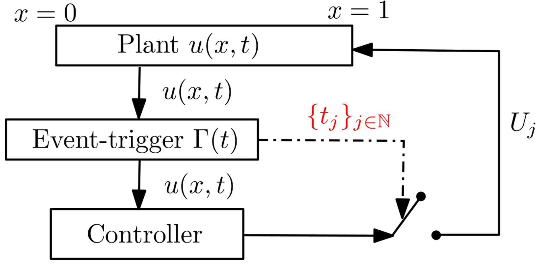
Refer to caption
Fig. 1: Event-triggered closed-loop system.

Let us now present the event-triggered boundary control approach considered in this work. It consists of two components: 1) a dynamic event-triggering mechanism which decides the time instants at which the control value needs to be sampled/updated and 2) the infinite-dimensional backstepping boundary control applied in a Zero-order hold fashion. The structure of the closed-loop system consisting of the plant, controller, and the event trigger is illustrated in Fig. 1.

Definition 1:

Let η,γ,ρ,β1,β2>0\eta,\gamma,\rho,\beta_{1},\beta_{2}>0. The event-triggered boundary control strategy consists of two components.

  1. 1.

    (The control action) The event-triggered boundary control input

    Uj=∫01k⁡(y,tj)​u​(y,tj)​𝑑y,U_{j}=\int_{0}^{1}k(y,t_{j})u(y,t_{j})dy, (27)

    for all t∈[tj,tj+1),j∈ℕt\in[t_{j},t_{j+1}),j\in\mathbb{N} where k⁡(y,t)k(y,t) is given by (16).

  2. 2.

    (The event-trigger) The set of event times I={t0,t1,t2,…}I=\{t_{0},t_{1},t_{2},\ldots\} with t0=0t_{0}=0 forms an increasing sequence via the following rule:

    tj+1=inf{t∈ℝ+|t>tj,d2(t)>γm(t)}t_{j+1}=\inf\{t\in\mathbb{R}_{+}|t>t_{j},d^{2}(t)>\gamma m(t)\} (28)

    and m⁡(t)m(t) satisfies the ODE

    m˙​(t)=−η​m​(t)−ρ​d2​(t)+β1​‖u⁡[t]‖2+β2​|u⁡(1,t)|2,\begin{split}\dot{m}(t)=&-\eta m(t)-\rho d^{2}(t)+\beta_{1}\|u[t]\|^{2}+\beta_{2}|u(1,t)|^{2},\end{split} (29)

    for all t∈(tj,tj+1)t\in(t_{j},t_{j+1}) with m⁡(t0)=m⁡(0)>0m(t_{0})=m(0)>0 and m⁡(tj−)=m⁡(tj)=m⁡(tj+)m(t_{j}^{-})=m(t_{j})=m(t_{j}^{+}).

Lemma 1:

Under the definition of the event-trigger (28)-(29), it holds that d2​(t)≤γ​m​(t)d^{2}(t)\leq\gamma m(t) and m⁡(t)>0m(t)>0, for all t∈[0,sup(I))t\in[0,\sup(I)).

Proof: The proof is very similar to that of Lemma 1 in [12], and hence omitted. ■\hfill\blacksquare

Lemma 2:

For F⁡(t)F(t) given by (12), it holds that

F(n)​(t)=λ(n)​(t)ε​e∫0tλ⁡(ξ)​𝑑ξ+∑m=1nn!(n−m)!​m!λ(n−m)(t)F(m−1)(t),\begin{split}F^{(n)}(t)=&\frac{\lambda^{(n)}(t)}{\varepsilon}e^{\int_{0}^{t}\lambda(\xi)d\xi}\\ &+\sum_{m=1}^{n}\frac{n!}{(n-m)!m!}\lambda^{(n-m)}(t)F^{(m-1)}(t),\end{split} (30)

for any n∈ℕ​\​{0}n\in\mathbb{N}\text{\textbackslash}\{0\}. Further, let λ⁡(t)\lambda(t) satisfy Assumption 1. Then, it holds that

|F(n)​(t)|≤(n+1)!​Dn+1ε​e∫0tλ⁡(ξ)​𝑑ξ,|F^{(n)}(t)|\leq\frac{(n+1)!D^{n+1}}{\varepsilon}e^{\int_{0}^{t}\lambda(\xi)d\xi}, (31)

for any n∈ℕn\in\mathbb{N}.

Proof: From mathematical induction, we can easily show that (30) holds for all n=1,2,…n=1,2,\ldots. For n=0n=0, due to Assumption 1, we have that

|F(0)​(t)|=|F⁡(t)|≤Dε​e∫0tλ⁡(ξ)​𝑑ξ,|F^{(0)}(t)|=|F(t)|\leq\frac{D}{\varepsilon}e^{\int_{0}^{t}\lambda(\xi)d\xi}, (32)

and thus, relation (31) holds for n=0n=0. For any n∈ℕ​\​{0}n\in\mathbb{N}\text{\textbackslash}\{0\}, we can write from (30) that

|F(n)​(t)|≤|λ(n)​(t)|ε​e∫0tλ⁡(ξ)​𝑑ξ+∑m=1nn!(n−m)!​m!|λ(n−m)(t)|⋅|F(m−1)(t)|.\begin{split}|F^{(n)}(t)|\leq&\frac{|\lambda^{(n)}(t)|}{\varepsilon}e^{\int_{0}^{t}\lambda(\xi)d\xi}\\ &+\sum_{m=1}^{n}\frac{n!}{(n-m)!m!}|\lambda^{(n-m)}(t)|\cdot|F^{(m-1)}(t)|.\end{split} (33)

Let us assume that the relation (31) holds for all n=1,…,n−1n=1,\ldots,n-1. Then, using Assumption 1, we can obtain from (33) that

|Fn​(t)|≤Dn+1​n!ε​e∫0tλ⁡(ξ)​𝑑ξ+Dn+1ε​e∫0tλ⁡(ξ)​𝑑ξ​∑m=1nn!≤Dn+1​n!ε​e∫0tλ⁡(ξ)​𝑑ξ+n​Dn+1​n!ε​e∫0tλ⁡(ξ)​𝑑ξ≤(n+1)!​Dn+1ε​e∫0tλ⁡(ξ)​𝑑ξ,\begin{split}|F^{n}(t)|\leq&\frac{D^{n+1}n!}{\varepsilon}e^{\int_{0}^{t}\lambda(\xi)d\xi}+\frac{D^{n+1}}{\varepsilon}e^{\int_{0}^{t}\lambda(\xi)d\xi}\sum_{m=1}^{n}n!\\ \leq&\frac{D^{n+1}n!}{\varepsilon}e^{\int_{0}^{t}\lambda(\xi)d\xi}+n\frac{D^{n+1}n!}{\varepsilon}e^{\int_{0}^{t}\lambda(\xi)d\xi}\\ \leq&\frac{(n+1)!D^{n+1}}{\varepsilon}e^{\int_{0}^{t}\lambda(\xi)d\xi},\end{split} (34)

which completes the proof. ■\hfill\blacksquare

Lemma 3:

Let the solution to the gain kernel equations (5a)-(5c) be given by (11). Then, subject to Assumption 1, the following bounds can be obtained for all 0≤y≤x≤10\leq y\leq x\leq 1 and t≥0t\geq 0.:

|K⁡(x,y,t)|\displaystyle|K(x,y,t)| ≤D2​ε​eD4​ε,\displaystyle\leq\frac{D}{2\varepsilon}e^{\frac{D}{4\varepsilon}}, (35)
|Kt​(x,y,t)|\displaystyle|K_{t}(x,y,t)| ≤D22​ε​(3+D4​ε)​eD4​ε,\displaystyle\leq\frac{D^{2}}{2\varepsilon}\Big(3+\frac{D}{4\varepsilon}\Big)e^{\frac{D}{4\varepsilon}}, (36)
|Kx​(x,y,t)|\displaystyle|K_{x}(x,y,t)| ≤D2​ε​(1+D2​ε)​eD4​ε,\displaystyle\leq\frac{D}{2\varepsilon}\Big(1+\frac{D}{2\varepsilon}\Big)e^{\frac{D}{4\varepsilon}}, (37)
|Kx​t​(x,y,t)|\displaystyle|K_{xt}(x,y,t)| ≤D2ε​(32+9​D8​ε+D216​ε2)​eD4​ε,\displaystyle\leq\frac{D^{2}}{\varepsilon}\Big(\frac{3}{2}+\frac{9D}{8\varepsilon}+\frac{D^{2}}{16\varepsilon^{2}}\Big)e^{\frac{D}{4\varepsilon}}, (38)
|Kx​y​(x,y,t)|\displaystyle|K_{xy}(x,y,t)| ≤D24​ε2​(1+D2​ε)​eD4​ε,\displaystyle\leq\frac{D^{2}}{4\varepsilon^{2}}\Big(1+\frac{D}{2\varepsilon}\Big)e^{\frac{D}{4\varepsilon}}, (39)
|Ky​(x,y,t)|\displaystyle|K_{y}(x,y,t)| ≤D24​ε2​eD4​ε,\displaystyle\leq\frac{D^{2}}{4\varepsilon^{2}}e^{\frac{D}{4\varepsilon}}, (40)
|Ky​y​(x,y,t)|\displaystyle|K_{yy}(x,y,t)| ≤D24​ε2​(1+D2​ε)​eD4​ε,\displaystyle\leq\frac{D^{2}}{4\varepsilon^{2}}\Big(1+\frac{D}{2\varepsilon}\Big)e^{\frac{D}{4\varepsilon}}, (41)
|Kx​y​y​(x,y,t)|\displaystyle|K_{xyy}(x,y,t)| ≤D24​ε2​(1+D2​ε+D24​ε2)​eD4​ε,\displaystyle\leq\frac{D^{2}}{4\varepsilon^{2}}\Big(1+\frac{D}{2\varepsilon}+\frac{D^{2}}{4\varepsilon^{2}}\Big)e^{\frac{D}{4\varepsilon}}, (42)

Proof: Due to page limitations, we will only provide the derivations of the relations (35)-(37). The rest of the results can be obtained by following the same arguments used to derive (35)-(37).

Using (11), relation (31) in Lemma 2, and the fact that 0≤y≤x≤10\leq y\leq x\leq 1, we can obtain that

|K⁡(x,y,t)|≤D2​ε​∑n=0∞1n!​((x2−y2)​D4​ε)n≤D2​ε​e(x2−y2)​D4​ε≤D2​ε​eD4​ε.\begin{split}|K(x,y,t)|&\leq\frac{D}{2\varepsilon}\sum_{n=0}^{\infty}\frac{1}{n!}\Big(\frac{(x^{2}-y^{2})D}{4\varepsilon}\Big)^{n}\\ &\leq\frac{D}{2\varepsilon}e^{\frac{(x^{2}-y^{2})D}{4\varepsilon}}\leq\frac{D}{2\varepsilon}e^{\frac{D}{4\varepsilon}}.\end{split} (43)

Differentiating (11) with respect to tt, we can obtain that

Kt​(x,y,t)=x2λ(t)e−∫0tλ(ξ)dξ∑n=0∞1n!​(n+1)!(x2−y24​ε)nF(n)(t)−x2e−∫0tλ(ξ)dξ∑n=0∞1n!​(n+1)!(x2−y24​ε)nF(n+1)(t).\begin{split}&K_{t}(x,y,t)\\ &=\frac{x}{2}\lambda(t)e^{-\int_{0}^{t}\lambda(\xi)d\xi}\sum_{n=0}^{\infty}\frac{1}{n!(n+1)!}\Big(\frac{x^{2}-y^{2}}{4\varepsilon}\Big)^{n}F^{(n)}(t)\\ &-\frac{x}{2}e^{-\int_{0}^{t}\lambda(\xi)d\xi}\sum_{n=0}^{\infty}\frac{1}{n!(n+1)!}\Big(\frac{x^{2}-y^{2}}{4\varepsilon}\Big)^{n}F^{(n+1)}(t).\end{split} (44)

Using Assumption 1, relation (31) in Lemma 2, and the fact that 0≤y≤x≤10\leq y\leq x\leq 1, we can obtain that

|Kt​(x,y,t)|≤D22​ε​∑n=0∞1n!​((x2−y2)​D4​ε)n+D22​ε∑n=0∞n+2n!((x2−y2)​D4​ε)n≤3​D22​ε​∑n=0∞1n!​((x2−y2)​D4​ε)n+D22​ε(x2−y2)​D4​ε∑n=1∞1(n−1)!((x2−y2)​D4​ε)n−1≤3​D22​ε​e(x2−y2)​D4​ε+D3​(x2−y2)8​ε2​e(x2−y2)​D4​ε≤D22​ε​(3+D4​ε)​eD4​ε.\begin{split}&|K_{t}(x,y,t)|\leq\frac{D^{2}}{2\varepsilon}\sum_{n=0}^{\infty}\frac{1}{n!}\Big(\frac{(x^{2}-y^{2})D}{4\varepsilon}\Big)^{n}\\ &\quad+\frac{D^{2}}{2\varepsilon}\sum_{n=0}^{\infty}\frac{n+2}{n!}\Big(\frac{(x^{2}-y^{2})D}{4\varepsilon}\Big)^{n}\\ &\leq\frac{3D^{2}}{2\varepsilon}\sum_{n=0}^{\infty}\frac{1}{n!}\Big(\frac{(x^{2}-y^{2})D}{4\varepsilon}\Big)^{n}\\ &\quad+\frac{D^{2}}{2\varepsilon}\frac{(x^{2}-y^{2})D}{4\varepsilon}\sum_{n=1}^{\infty}\frac{1}{(n-1)!}\Big(\frac{(x^{2}-y^{2})D}{4\varepsilon}\Big)^{n-1}\\ &\leq\frac{3D^{2}}{2\varepsilon}e^{\frac{(x^{2}-y^{2})D}{4\varepsilon}}+\frac{D^{3}(x^{2}-y^{2})}{8\varepsilon^{2}}e^{\frac{(x^{2}-y^{2})D}{4\varepsilon}}\\ &\leq\frac{D^{2}}{2\varepsilon}\Big(3+\frac{D}{4\varepsilon}\Big)e^{\frac{D}{4\varepsilon}}.\end{split} (45)

Differentiating (11) with respect to xx, we can obtain that

Kx​(x,y,t)=−12e−∫0tλ(ξ)dξ∑n=0∞1n!​(n+1)!(x2−y24​ε)nF(n)(t)−x24​εe−∫0tλ(ξ)dξ∑n=1∞1(n−1)!​(n+1)!(x2−y24​ε)n−1×F(n)​(t).\begin{split}&K_{x}(x,y,t)\\ &=-\frac{1}{2}e^{-\int_{0}^{t}\lambda(\xi)d\xi}\sum_{n=0}^{\infty}\frac{1}{n!(n+1)!}\Big(\frac{x^{2}-y^{2}}{4\varepsilon}\Big)^{n}F^{(n)}(t)\\ &-\frac{x^{2}}{4\varepsilon}e^{-\int_{0}^{t}\lambda(\xi)d\xi}\sum_{n=1}^{\infty}\frac{1}{(n-1)!(n+1)!}\Big(\frac{x^{2}-y^{2}}{4\varepsilon}\Big)^{n-1}\\ &\qquad\qquad\qquad\qquad\quad\times F^{(n)}(t).\end{split} (46)

Using Assumption 1, relation (31) in Lemma 2, and the fact that 0≤y≤x≤10\leq y\leq x\leq 1, we can obtain that

|Kx​(x,y,t)|≤D2​ε​∑n=0∞1n!​((x2−y2)​D4​ε)n+D24​ε2∑n=1∞1(n−1)!((x2−y2)​D4​ε)n−1≤D2​ε​e(x2−y2)​D4​ε+D24​ε2​e(x2−y2)​D4​ε≤D2​ε​(1+D2​ε)​eD4​ε.\begin{split}|K_{x}(x,y,t)|\leq&\frac{D}{2\varepsilon}\sum_{n=0}^{\infty}\frac{1}{n!}\Big(\frac{(x^{2}-y^{2})D}{4\varepsilon}\Big)^{n}\\ &+\frac{D^{2}}{4\varepsilon^{2}}\sum_{n=1}^{\infty}\frac{1}{(n-1)!}\Big(\frac{(x^{2}-y^{2})D}{4\varepsilon}\Big)^{n-1}\\ \leq&\frac{D}{2\varepsilon}e^{\frac{(x^{2}-y^{2})D}{4\varepsilon}}+\frac{D^{2}}{4\varepsilon^{2}}e^{\frac{(x^{2}-y^{2})D}{4\varepsilon}}\\ \leq&\frac{D}{2\varepsilon}\Big(1+\frac{D}{2\varepsilon}\Big)e^{\frac{D}{4\varepsilon}}.\end{split} (47)

■\hfill\blacksquare

Remark 3:

For the solution to the gain kernel equations (10a)-(10c) given by (13), we can obtain bounds similar to (35)-(42). However, we only require to know the bound for |L⁡(x,y,t)||L(x,y,t)| for 0≤y≤x≤10\leq y\leq x\leq 1 and t≥0t\geq 0. Similar to (35), we can show that L⁡(x,y,t)L(x,y,t) satisfies

|L⁡(x,y,t)|≤D2​ε​eD4​ε,|L(x,y,t)|\leq\frac{D}{2\varepsilon}e^{\frac{D}{4\varepsilon}}, (48)

for all 0≤y≤x≤10\leq y\leq x\leq 1 and t≥0t\geq 0.

Lemma 4:

For d⁡(t)d(t) given by (18), it holds that

d˙2(t)≤ρ1d2(t)+α1∥u[t]∥2+α2u(1,t)|2,\dot{d}^{2}(t)\leq\rho_{1}d^{2}(t)+\alpha_{1}\|u[t]\|^{2}+\alpha_{2}u(1,t)|^{2}, (49)

for some ρ1,α1,α2>0,\rho_{1},\alpha_{1},\alpha_{2}>0, for all t∈(tj,tj+1),j∈ℕ.t\in(t_{j},t_{j+1}),j\in\mathbb{N}.

Proof: Taking the time derivative of (18) between t∈(tj,tj+1),j∈ℕt\in(t_{j},t_{j+1}),j\in\mathbb{N} along the solution of (1a),(1b),(17),(27) and using integration by parts twice, we can obtain that

d˙(t)=−∫01kt(y,t)u(y,t)dy−∫01k(y,t)ut(y,t)dy=−∫01kt(y,t)u(y,t)dy−λ(t)∫01k(y,t)u(y,t)dy−ε​k​(1,t)​ux​(1,t)+ε​k​(0,t)​ux​(0,t)+ε​ky​(1,t)​u​(1,t)−ε​ky​(0,t)​u​(0,t)−ε​∫01ky​y​(y,t)​u​(y,t)​dy.\begin{split}&\dot{d}(t)=-\int_{0}^{1}k_{t}(y,t)u(y,t)dy-\int_{0}^{1}k(y,t)u_{t}(y,t)dy\\ &=-\int_{0}^{1}k_{t}(y,t)u(y,t)dy-\lambda(t)\int_{0}^{1}k(y,t)u(y,t)dy\\ &\quad-\varepsilon k(1,t)u_{x}(1,t)+\varepsilon k(0,t)u_{x}(0,t)+\varepsilon k_{y}(1,t)u(1,t)\\ &\quad-\varepsilon k_{y}(0,t)u(0,t)-\varepsilon\int_{0}^{1}k_{yy}(y,t)u(y,t)dy.\end{split} (50)

Note that we can show from (11) and (16) that ky​(0,t)=0k_{y}(0,t)=0. Further note that ux​(0,t)=0u_{x}(0,t)=0 and

ux​(1,t)=−q​u​(1,t)+Uj=−q​u​(1,t)+d⁡(t)+∫01k⁡(y,t)​u​(y,t)​𝑑y\begin{split}u_{x}(1,t)&=-qu(1,t)+U_{j}\\ &=-qu(1,t)+d(t)+\int_{0}^{1}k(y,t)u(y,t)dy\end{split} (51)

from (17) and (27). Thus, we can rewrite (50) as

d˙​(t)=−ε​k​(1,t)​d​(t)+ε⁡(q​k​(1,t)+ky​(1,t))​u​(1,t)−∫01(kt(y,t)+λ(t)k(y,t)+εk(1,t)k(y,t)OPENOPEN+ε​ky​y​(y,t)))​u​(y,t)​d​y,\begin{split}&\dot{d}(t)=-\varepsilon k(1,t)d(t)+\varepsilon\big(qk(1,t)+k_{y}(1,t)\big)u(1,t)\\ &-\int_{0}^{1}\Big(k_{t}(y,t)+\lambda(t)k(y,t)+\varepsilon k(1,t)k(y,t)\\ &\qquad\qquad\qquad\qquad\qquad+\varepsilon k_{yy}(y,t)\big)\Big)u(y,t)dy,\end{split} (52)

from which we can obtain using Assumption 1 and Cauchy-Schwarz inequality that

|d˙​(t)|≤ε​maxt≥0⁡(|k⁡(1,t)|)|d⁡(t)|+ε⁡(q​maxt≥0​|k⁡(1,t)|CLOSEOPEN+maxt≥0⁡|ky​(1,t)|)​|u⁡(1,t)|+(maxt≥0,y∈[0,1]⁡|kt​(y,t)|+D​maxt≥0,y∈[0,1]​|k⁡(y,t)|CLOSE+ε​maxt≥0​|k⁡(1,t)|​maxt≥0,y∈[0,1]​|k⁡(y,t)|OPEN+ε​maxt≥0,y∈[0,1]​|ky​y​(y,t)|)​‖u⁡[t]‖.\begin{split}&|\dot{d}(t)|\\ &\leq\varepsilon\max_{t\geq 0}\big(|k(1,t)|\big)|d(t)|+\varepsilon\Big(q\max_{t\geq 0}|k(1,t)|\\ &\qquad\qquad+\max_{t\geq 0}|k_{y}(1,t)|\Big)|u(1,t)|\\ &+\Big(\max_{t\geq 0,y\in[0,1]}|k_{t}(y,t)|+D\max_{t\geq 0,y\in[0,1]}|k(y,t)|\\ &\qquad+\varepsilon\max_{t\geq 0}|k(1,t)|\max_{t\geq 0,y\in[0,1]}|k(y,t)|\\ &\qquad+\varepsilon\max_{t\geq 0,y\in[0,1]}|k_{yy}(y,t)|\Big)\|u[t]\|.\end{split} (53)

As r⁡(t)=q−λ⁡(t)2​εr(t)=q-\frac{\lambda(t)}{2\varepsilon}, using Assumption 1, we can show that

|r⁡(t)|≤q+D2​ε,|r(t)|\leq q+\frac{D}{2\varepsilon}, (54)

and

|r˙​(t)|≤D22​ε.|\dot{r}(t)|\leq\frac{D^{2}}{2\varepsilon}. (55)

Considering (16),(35)-(42),(54),(55), we can obtain the following relations:

|kt​(y,t)|≤|Kx​t​(1,y,t)|+|r˙​(t)|⋅|K⁡(1,y,t)|+|r(t)|⋅|Kt(1,y,t)|≤|Kx​t​(1,y,t)|+D22​ε​|K⁡(1,y,t)|+(q+D2​ε)​|Kt​(1,y,t)|≤max0≤y≤x≤1⁡(|Kx​t​(x,y,t)|+D22​ε​|K⁡(x,y,t)|CLOSEOPEN+(q+D2​ε)​|Kt​(x,y,t)|)≤D2ε​(32+3​q2+q​D8​ε+17​D8​ε+D28​ε2)​eD4​ε,\begin{split}&|k_{t}(y,t)|\leq|K_{xt}(1,y,t)|+|\dot{r}(t)|\cdot|K(1,y,t)|\\ &\qquad\qquad\qquad\qquad\qquad\qquad+|r(t)|\cdot|K_{t}(1,y,t)|\\ &\leq|K_{xt}(1,y,t)|+\frac{D^{2}}{2\varepsilon}|K(1,y,t)|+\Big(q+\frac{D}{2\varepsilon}\Big)|K_{t}(1,y,t)|\\ &\leq\max_{0\leq y\leq x\leq 1}\Big(|K_{xt}(x,y,t)|+\frac{D^{2}}{2\varepsilon}|K(x,y,t)|\\ &\qquad\qquad\qquad\qquad\qquad\qquad+\Big(q+\frac{D}{2\varepsilon}\Big)|K_{t}(x,y,t)|\Big)\\ &\leq\frac{D^{2}}{\varepsilon}\Big(\frac{3}{2}+\frac{3q}{2}+\frac{qD}{8\varepsilon}+\frac{17D}{8\varepsilon}+\frac{D^{2}}{8\varepsilon^{2}}\Big)e^{\frac{D}{4\varepsilon}},\end{split} (56)
|k⁡(y,t)|≤|Kx​(1,y,t)|+|r⁡(t)|⋅|K⁡(1,y,t)|≤max0≤y≤x≤1⁡(|Kx​(x,y,t)|+(q+D2​ε)​|K⁡(x,y,t)|)≤D2​ε​(1+q+Dε)​eD4​ε,\begin{split}&|k(y,t)|\leq|K_{x}(1,y,t)|+|r(t)|\cdot|K(1,y,t)|\\ &\leq\max_{0\leq y\leq x\leq 1}\Big(|K_{x}(x,y,t)|+\Big(q+\frac{D}{2\varepsilon}\Big)|K(x,y,t)|\Big)\\ &\leq\frac{D}{2\varepsilon}\Big(1+q+\frac{D}{\varepsilon}\Big)e^{\frac{D}{4\varepsilon}},\end{split} (57)
|ky​(y,t)|≤|Kx​y​(1,y,t)|+|r⁡(t)|⋅|Ky​(1,y,t)|≤max0≤y≤x≤1⁡(|Kx​y​(x,y,t)|+(q+D2​ε)​|Ky​(x,y,t)|)≤D24​ε2​(1+q+Dε)​eD4​ε,\begin{split}&|k_{y}(y,t)|\leq|K_{xy}(1,y,t)|+|r(t)|\cdot|K_{y}(1,y,t)|\\ &\leq\max_{0\leq y\leq x\leq 1}\Big(|K_{xy}(x,y,t)|+\Big(q+\frac{D}{2\varepsilon}\Big)|K_{y}(x,y,t)|\Big)\\ &\leq\frac{D^{2}}{4\varepsilon^{2}}\Big(1+q+\frac{D}{\varepsilon}\Big)e^{\frac{D}{4\varepsilon}},\end{split} (58)

and

|ky​y​(y,t)|≤|Kx​y​y​(1,y,t)|+|r⁡(t)|⋅|Ky​y​(1,y,t)|≤max0≤y≤x≤1⁡(|Kx​y​y​(x,y,t)|+(q+D2​ε)​|Ky​y​(x,y,t)|)≤D24​ε2​(1+q+q​D2​ε+Dε+D22​ε2)​eD4​ε.\begin{split}&|k_{yy}(y,t)|\leq|K_{xyy}(1,y,t)|+|r(t)|\cdot|K_{yy}(1,y,t)|\\ &\leq\max_{0\leq y\leq x\leq 1}\Big(|K_{xyy}(x,y,t)|+\Big(q+\frac{D}{2\varepsilon}\Big)|K_{yy}(x,y,t)|\Big)\\ &\leq\frac{D^{2}}{4\varepsilon^{2}}\Big(1+q+\frac{qD}{2\varepsilon}+\frac{D}{\varepsilon}+\frac{D^{2}}{2\varepsilon^{2}}\Big)e^{\frac{D}{4\varepsilon}}.\end{split} (59)

Using Young’s inequality and (56)-(59), we can obtain from (53) that

d˙2​(t)≤ρ1​d2​(t)+α1​‖u⁡[t]‖2+α2​u2​(1,t)\dot{d}^{2}(t)\leq\rho_{1}d^{2}(t)+\alpha_{1}\|u[t]\|^{2}+\alpha_{2}u^{2}(1,t) (60)

where

ρ1=3​D24​(1+q+Dε)2​eD2​ε,\rho_{1}=\frac{3D^{2}}{4}\Big(1+q+\frac{D}{\varepsilon}\Big)^{2}e^{\frac{D}{2\varepsilon}}, (61)
α1=3​D4ε2​(94+9​q4+4​Dε+9​D8​ε+D24​ε2CLOSEOPEN+14​(1+q+Dε)2​eD4​ε)2​eD2​ε,\begin{split}&\alpha_{1}=\frac{3D^{4}}{\varepsilon^{2}}\bigg(\frac{9}{4}+\frac{9q}{4}+\frac{4D}{\varepsilon}+\frac{9D}{8\varepsilon}+\frac{D^{2}}{4\varepsilon^{2}}\\ &\qquad\qquad\qquad\qquad+\frac{1}{4}\Big(1+q+\frac{D}{\varepsilon}\Big)^{2}e^{\frac{D}{4\varepsilon}}\bigg)^{2}\ e^{\frac{D}{2\varepsilon}},\end{split} (62)
α2=3​D24​(q+D2​ε)2​(1+q+Dε)2​eD2​ε.\alpha_{2}=\frac{3D^{2}}{4}\Big(q+\frac{D}{2\varepsilon}\Big)^{2}\Big(1+q+\frac{D}{\varepsilon}\Big)^{2}e^{\frac{D}{2\varepsilon}}. (63)

This completes the proof. ■\hfill\blacksquare

Theorem 2:

Under the event-triggered boundary control in Definition 1, with β1,β2\beta_{1},\beta_{2} chosen as

β1=α1γ⁡(1−σ),β2=α2γ⁡(1−σ),\beta_{1}=\frac{\alpha_{1}}{\gamma(1-\sigma)},\hskip 5.0pt\beta_{2}=\frac{\alpha_{2}}{\gamma(1-\sigma)}, (64)

where α1,α2\alpha_{1},\alpha_{2} given by (62),(63) and σ∈(0,1)\sigma\in(0,1), there exists a minimal dwell-time τ>0\tau>0 between two triggering times, i.e., there exists a constant τ>0\tau>0 such that tj+1−tj≥τ,t_{j+1}-t_{j}\geq\tau, for all j∈ℕj\in\mathbb{N}, which is independent of the initial conditions and only depends on the system and control parameters.

Proof: The proof is very similar to that of Theorem 1 in [12], and hence omitted.

Corollary 1:

Under Assumption 1, for every u⁡[0]∈L2​(0,1)u[0]\in L^{2}(0,1), there exist unique solution u:ℝ+×[0,1]→ℝu:\mathbb{R}_{+}\times[0,1]\rightarrow\mathbb{R} such that u∈C0​(ℝ+;L2​(0,1)∩C1​(J×[0,1])CLOSEu\in C^{0}(\mathbb{R}_{+};L^{2}(0,1)\cap C^{1}(J\times[0,1]) with u⁡[t]∈C2​([0,1])u[t]\in C^{2}([0,1]) which satisfy (1b),(17) all t>0t>0 and (1a) for all t>0,x∈(0,1),t>0,x\in(0,1), where J=ℝ+​\​{tj≥0,j∈ℕ}J=\mathbb{R_{+}}\text{\textbackslash}\{t_{j}\geq 0,j\in\mathbb{N}\}. The increasing sequence {tj≥0,j∈ℕ}\{t_{j}\geq 0,j\in\mathbb{N}\} is determined by the set of rules given in Definition 1.

Proof: This is a straightforward consequence of Theorem 1 and 2. The solutions are constructed iteratively between successive triggering times. ■\hfill\blacksquare

Theorem 3:

Let γ,η>0\gamma,\eta>0 be design parameters, and β1,β2\beta_{1},\beta_{2} are chosen according to (64). Subject to Assumption 2, the parameter ρ>0\rho>0 is set as

ρ=ε​κ​B2,\rho=\frac{\varepsilon\kappa B}{2}, (65)

for B,κ>0B,\kappa>0 are chosen such that

B⁡(ε​min⁡{q−D2​ε−12,12}CLOSEOPEN−ε2​κ)−2​β1​(1+D2​ε​eD4​ε)2−2​β2−β2​D2ε2​eD2​ε>0.\begin{split}B\bigg(\varepsilon\min\Big\{q-\frac{D}{2\varepsilon}-\frac{1}{2},\frac{1}{2}\Big\}&-\frac{\varepsilon}{2\kappa}\bigg)-2\beta_{1}\Big(1+\frac{D}{2\varepsilon}e^{\frac{D}{4\varepsilon}}\Big)^{2}\\ &-2\beta_{2}-\frac{\beta_{2}D^{2}}{\varepsilon^{2}}e^{\frac{D}{2\varepsilon}}>0.\end{split} (66)

Note from Assumption 2 that q−D/2​ε>1/2q-D/2\varepsilon>1/2. Then, under Assumption 1 and 2, the closed-loop system which consists of the plant and the event-triggered boundary controller (28)-(27) has a unique solution and globally exponentially converges to zero, i.e., ‖u⁡[t]‖→0\|u[t]\|\rightarrow 0 as t→∞.t\rightarrow\infty.

Proof: From Corollary 1, the existence and the uniqueness of solutions to the system (1a),(1b),(17) under the event-triggered boundary control in Definition 1 is guaranteed. Now let us show that the closed- loop system is globally L2L^{2}-exponentially convergent to zero.

Let us choose the following candidate Lyapunov function noting that m⁡(t)>0m(t)>0 for all t≥0t\geq 0:

V=B2​∫01w2​(x,t)​𝑑x+m⁡(t),V=\frac{B}{2}\int_{0}^{1}w^{2}(x,t)dx+m(t), (67)

where B>0B>0 is chosen to satisfy (66). Differentiating (67) along the solution of (19a)-(19c) and (29), and using integration by parts twice, we can obtain that

V˙​(t)=−ε​B​r​(t)​w2​(1,t)+ε​B​d​(t)​w​(1,t)−ε​B​‖wx​[t]‖2−η​m​(t)−ρ​d2​(t)+β1​‖u⁡[t]‖2+β2​u2​(1,t).\begin{split}&\dot{V}(t)=-\varepsilon Br(t)w^{2}(1,t)+\varepsilon Bd(t)w(1,t)\\ &-\varepsilon B\|w_{x}[t]\|^{2}-\eta m(t)-\rho d^{2}(t)+\beta_{1}\|u[t]\|^{2}+\beta_{2}u^{2}(1,t).\end{split} (68)

From Young’s inequality, we can write that

ε​B​d​(t)​w​(1,t)=ε​B2​κ​w2​(1,t)+ε​κ​B2​d2​(t),\varepsilon Bd(t)w(1,t)=\frac{\varepsilon B}{2\kappa}w^{2}(1,t)+\frac{\varepsilon\kappa B}{2}d^{2}(t), (69)

for κ>0\kappa>0 chosen to satisfy (66). Furthermore, from Poincare’s inequality, we have that

‖w⁡[t]‖2≤2​w2​(1,t)+4​‖wx​[t]‖2.\|w[t]\|^{2}\leq 2w^{2}(1,t)+4\|w_{x}[t]\|^{2}. (70)

Thus, using (69),(70), we can obtain from (68) that

V˙≤−ε​B​r​(t)​w2​(1,t)+ε​B2​κ​w2​(1,t)+ε​B​κ2​d2​(t)+ε​B​(12​w2​(1,t)−14​‖w⁡[t]‖2)−η​m​(t)−ρ​d2​(t)+β1​‖u⁡[t]‖2+β2​u2​(1,t).\begin{split}&\dot{V}\leq-\varepsilon Br(t)w^{2}(1,t)+\frac{\varepsilon B}{2\kappa}w^{2}(1,t)+\frac{\varepsilon B\kappa}{2}d^{2}(t)\\ &+\varepsilon B\Big(\frac{1}{2}w^{2}(1,t)-\frac{1}{4}\|w[t]\|^{2}\Big)-\eta m(t)-\rho d^{2}(t)\\ &+\beta_{1}\|u[t]\|^{2}+\beta_{2}u^{2}(1,t).\end{split} (71)

Recalling (65), we can rewrite (71) as

V˙≤−ε​B​((r⁡(t)−12)−12​κ)​w2​(1,t)−ε​B4​‖w⁡[t]‖2−η​m​(t)+β1​‖u⁡[t]‖2+β2​u2​(1,t).\begin{split}&\dot{V}\leq-\varepsilon B\Big(\big(r(t)-\frac{1}{2}\big)-\frac{1}{2\kappa}\Big)w^{2}(1,t)-\frac{\varepsilon B}{4}\|w[t]\|^{2}\\ &-\eta m(t)+\beta_{1}\|u[t]\|^{2}+\beta_{2}u^{2}(1,t).\end{split} (72)

Using Young’s inequality and Cauchy-Schwarz inequality, we can obtain from (9) that

u2​(1,t)≤2​w2​(1,t)+2​∫01L2​(1,y,t)​dy​‖w⁡[t]‖2,\begin{split}u^{2}(1,t)&\leq 2w^{2}(1,t)+2\int_{0}^{1}L^{2}(1,y,t)dy\|w[t]\|^{2},\end{split} (73)

and

‖u⁡[t]‖2≤(1+(∫01∫0xL2​(x,y)​𝑑y​𝑑x)1/2)2​‖w⁡[t]‖2.\|u[t]\|^{2}\leq\bigg(1+\Big(\int_{0}^{1}\int_{0}^{x}L^{2}(x,y)dydx\Big)^{1/2}\bigg)^{2}\|w[t]\|^{2}. (74)

Thus, recalling Remark 3, we can show that

u2​(1,t)=2​w2​(1,t)+D22​ε2​eD2​ε​‖w⁡[t]‖2,u^{2}(1,t)=2w^{2}(1,t)+\frac{D^{2}}{2\varepsilon^{2}}e^{\frac{D}{2\varepsilon}}\|w[t]\|^{2}, (75)

and

‖u⁡[t]‖2≤(1+D2​ε​eD4​ε)2​‖w⁡[t]‖2.\begin{split}\|u[t]\|^{2}\leq\bigg(1+\frac{D}{2\varepsilon}e^{\frac{D}{4\varepsilon}}\bigg)^{2}\|w[t]\|^{2}.\end{split} (76)

Therefore, we can obtain from (72) as

V˙≤−(ε​B​((r⁡(t)−12)−12​κ)−2​β2)​w2​(1,t)−(ε​B4−β1​(1+D2​ε​eD4​ε)−β2​D22​ε2​eD2​ε)​‖w⁡[t]‖2−η​m​(t).\begin{split}&\dot{V}\leq-\bigg(\varepsilon B\Big(\big(r(t)-\frac{1}{2}\big)-\frac{1}{2\kappa}\Big)-2\beta_{2}\bigg)w^{2}(1,t)\\ &-\bigg(\frac{\varepsilon B}{4}-\beta_{1}\Big(1+\frac{D}{2\varepsilon}e^{\frac{D}{4\varepsilon}}\Big)-\frac{\beta_{2}D^{2}}{2\varepsilon^{2}}e^{\frac{D}{2\varepsilon}}\bigg)\|w[t]\|^{2}-\eta m(t).\end{split} (77)

Considering Assumption 1 and 2, and equation (8), we can write that

r⁡(t)≥q−D2​ε>12.r(t)\geq q-\frac{D}{2\varepsilon}>\frac{1}{2}. (78)

Thus, we can rewrite (77) as

V˙≤−(ε​B​((q−D2​ε−12)−12​κ)−2​β2)​w2​(1,t)−(ε​B4−β1​(1+D2​ε​eD4​ε)−β2​D22​ε2​eD2​ε)2​‖w⁡[t]‖2−η​m​(t).\begin{split}&\dot{V}\leq-\bigg(\varepsilon B\Big(\big(q-\frac{D}{2\varepsilon}-\frac{1}{2}\big)-\frac{1}{2\kappa}\Big)-2\beta_{2}\bigg)w^{2}(1,t)\\ &-\bigg(\frac{\varepsilon B}{4}-\beta_{1}\Big(1+\frac{D}{2\varepsilon}e^{\frac{D}{4\varepsilon}}\Big)-\frac{\beta_{2}D^{2}}{2\varepsilon^{2}}e^{\frac{D}{2\varepsilon}}\bigg)^{2}\|w[t]\|^{2}-\eta m(t).\end{split} (79)

Let

b1:=ε​B​((q−D2​ε−12)−12​κ)−2​β2,b_{1}:=\varepsilon B\Big(\big(q-\frac{D}{2\varepsilon}-\frac{1}{2}\big)-\frac{1}{2\kappa}\Big)-2\beta_{2}, (80)

and

b2:=ε​B4−β1​(1+D2​ε​eD4​ε)2−β2​D22​ε2​eD2​ε.b_{2}:=\frac{\varepsilon B}{4}-\beta_{1}\Big(1+\frac{D}{2\varepsilon}e^{\frac{D}{4\varepsilon}}\Big)^{2}-\frac{\beta_{2}D^{2}}{2\varepsilon^{2}}e^{\frac{D}{2\varepsilon}}. (81)

As B>0B>0 and κ>0\kappa>0 have been selected to satisfy (66), we can observe that b1,b2>0b_{1},b_{2}>0. Thus, considering (67), we can obtain from (79) that

V˙≤−2​ϱ​V,\dot{V}\leq-2\varrho V, (82)

where

ϱ=min⁡{b2B,η2},\varrho=\min\Big\{\frac{b_{2}}{B},\frac{\eta}{2}\Big\}, (83)

from which we can obtain using standard arguments that

V⁡(t)≤e−2​ϱ​t​V​(0).V(t)\leq e^{-2\varrho t}V(0). (84)

This implies due to (67) that ‖w⁡[t]‖→0\|w[t]\|\rightarrow 0 as t→∞t\rightarrow\infty. Therefore, considering (76), we can conclude that ‖u⁡[t]‖→0\|u[t]\|\rightarrow 0 as t→∞t\rightarrow\infty. This completes the proof. ■\hfill\blacksquare

IV Numerical Simulations

We consider a reaction-diffusion system with ε=1,λ⁡(t)=3/(1+t),t≥0,q=3,\varepsilon=1,\lambda(t)=3/(1+t),t\geq 0,q=3, and the initial conditions u⁡[0]=10​x2​(x−1)2u[0]=10x^{2}(x-1)^{2}. It is easy to show that λ⁡(t)\lambda(t) satisfies Assumption 1 with D=3D=3. The parameters for the event-trigger in Definition 1 are chosen as follows: m⁡(0)=10−4,γ=1,η=1,m(0)=10^{-4},\gamma=1,\eta=1, and σ=0.5\sigma=0.5. It can be shown using (62),(63) that α1=3.0084×10⁶,α2=3.9624×10³\alpha_{1}=3.0084\times 10^{6},\alpha_{2}=3.9624\times 10^{3}. Therefore, from (64), we can obtain β1=6.0167×10⁶;β2=7.9248×10³\beta_{1}=6.0167\times 10^{6};\beta_{2}=7.9248\times 10^{3}. Let us choose BB and κ\kappa as B=8.4054×10⁸B=8.4054\times 10^{8} and κ=2\kappa=2 so that (66) is satisfied. Then, from (65), we can obtain ρ=8.4054×10⁸\rho=8.4054\times 10^{8}.

Fig. 2 illustrates the evolution of event-triggered control (ETC) and continuous-time control (CTC) inputs. We can clearly observe that ETC significantly reduces the number of control updates compared to CTC. Fig. 3 shows the evolution of ‖u⁡[t]‖\|u[t]\|, and we can observe that the convergence under ETC is the fastest.

Refer to caption
Fig. 2: Event-triggered control (ETC) and continuous-time control (CTC) inputs.
Refer to caption
Fig. 3: Evolution of ‖u⁡[t]‖\|u[t]\|.

V Conclusion

This paper has proposed an event-triggered full-state feedback boundary control strategy for a class of reaction-diffusion systems with time-dependent reactivity under Robin boundary actuation. We have used a dynamic event triggering condition to determine when the control value needs to be updated. Under the proposed strategy, we have proved the existence of a uniform minimal-dwell time between two updates, which excludes Zeno behavior. Further, we have shown the well-posedness of the closed-loop system and its global L2L^{2}-exponential convergence to zero.

Appendix A
Solution to (5) and (10)

Let us make the following change of variables

K(x,y,t)=−x2e−∫0tλ(ξ)dξf(z,t), z=x2−y2,K(x,y,t)=-\frac{x}{2}e^{-\int_{0}^{t}\lambda(\xi)d\xi}f(z,t),\text{ }z=\sqrt{x^{2}-y^{2}}, (85)

from which we get the following PDE in one spatial variable for the function f⁡(z,t)f(z,t)

ft​(x,t)=ε​fz​z​(z,t)+3​εz​fz​(z,t),f_{t}(x,t)=\varepsilon f_{zz}(z,t)+\frac{3\varepsilon}{z}f_{z}(z,t), (86)

with the boundary conditions

fz​(0,t)\displaystyle f_{z}(0,t) =0,\displaystyle=0, (87)
f⁡(0,t)\displaystyle f(0,t) =λ⁡(t)ε​e∫0tλ⁡(ξ)​𝑑ξ.\displaystyle=\frac{\lambda(t)}{\varepsilon}e^{\int_{0}^{t}\lambda(\xi)d\xi}. (88)

We further make the following change of coordinates and variables

t¯=ε​t,\bar{t}=\varepsilon t, (89)

and

f¯​(z,t¯)=f​(z,t)\bar{f}(z,\bar{t})=f(z,t) (90)

from which we obtain the following PDE

f¯t¯​(z,t¯)\displaystyle\bar{f}_{\bar{t}}(z,\bar{t}) =f¯z​z​(z,t¯)+3z​f¯z​(z,t¯)\displaystyle=\bar{f}_{zz}(z,\bar{t})+\frac{3}{z}\bar{f}_{z}(z,\bar{t}) (91)
f¯z​(0,t¯)\displaystyle\bar{f}_{z}(0,\bar{t}) =0\displaystyle=0 (92)
f¯​(0,t¯)\displaystyle\bar{f}(0,\bar{t}) =λ⁡(t¯/ε)ε​e∫0t¯/ελ⁡(ξ)​𝑑ξ:=F⁡(t¯/ε)=F⁡(t).\displaystyle=\frac{\lambda(\bar{t}/\varepsilon)}{\varepsilon}e^{\int_{0}^{\bar{t}/\varepsilon}\lambda(\xi)d\xi}:=F(\bar{t}/\varepsilon)=F(t). (93)

The unique solution to (91)-(93) is given by [22]

f¯​(z,t¯)=f​(z,t)=∑n=0∞1n!​(n+1)!​(z24)n​dn​F​(t)d​t¯n=∑n=0∞1n!​(n+1)!​(z24​ε)n​F(n)​(t).\begin{split}\bar{f}(z,\bar{t})=f(z,t)=&\sum_{n=0}^{\infty}\frac{1}{n!(n+1)!}\Big(\frac{z^{2}}{4}\Big)^{n}\frac{d^{n}F(t)}{d\bar{t}^{n}}\\ =&\sum_{n=0}^{\infty}\frac{1}{n!(n+1)!}\Big(\frac{z^{2}}{4\varepsilon}\Big)^{n}F^{(n)}(t).\end{split} (94)

Thus, considering (85) and (94), we can obtain the closed-form solution (11) for all 0≤y≤x≤10\leq y\leq x\leq 1 and t≥0t\geq 0.

By comparing the PDEs (5a)-(5c) and (10a)-(10c), we can observe that

L⁡(x,y,t,λ⁡(t))=−K⁡(x,y,t,−λ⁡(t)),L\big(x,y,t;\lambda(t)\big)=-K\big(x,y,t;-\lambda(t)\big), (95)

from which we can show that the solution for L⁡(x,y,t)L(x,y,t) for all 0≤y≤x≤10\leq y\leq x\leq 1 and t≥0t\geq 0 is given by (13).

References

  • [1] W. Heemels, K. H. Johansson, and P. Tabuada, “An introduction to event-triggered and self-triggered control,” in 2012 51st IEEE Conference on Decision and Control (CDC). IEEE, 2012, pp. 3270–3285.
  • [2] L. Hetel, C. Fiter, H. Omran, A. Seuret, E. Fridman, J.-P. Richard, and S. I. Niculescu, “Recent developments on the stability of systems with aperiodic sampling: An overview,” Automatica, vol. 76, pp. 309–335, 2017.
  • [3] I. Karafyllis and M. Krstic, “Sampled-data boundary feedback control of 1-D linear transport PDEs with non-local terms,” Systems & Control Letters, vol. 107, pp. 68–75, 2017.
  • [4] ——, “Sampled-data boundary feedback control of 1-D parabolic PDEs,” Automatica, vol. 87, pp. 226–237, 2018.
  • [5] M. Lemmon, “Event-triggered feedback in control, estimation, and optimization,” Networked control systems, pp. 293–358, 2010.
  • [6] T. Liu and Z.-P. Jiang, “A small-gain approach to robust event-triggered control of nonlinear systems,” IEEE Transactions on Automatic Control, vol. 60, no. 8, pp. 2072–2085, 2015.
  • [7] N. Espitia, A. Girard, N. Marchand, and C. Prieur, “Event-based control of linear hyperbolic systems of conservation laws,” Automatica, vol. 70, pp. 275–287, 2016.
  • [8] N. Espitia, “Observer-based event-triggered boundary control of a linear 2×\times 2 hyperbolic systems,” Systems & Control Letters, vol. 138, p. 104668, 2020.
  • [9] N. Espitia, I. Karafyllis, and M. Krstic, “Event-triggered boundary control of constant-parameter reaction–diffusion PDEs: a small-gain approach,” Automatica, vol. 128, p. 109562, 2021.
  • [10] R. Katz, E. Fridman, and A. Selivanov, “Boundary delayed observer-controller design for reaction-diffusion systems,” IEEE Transactions on Automatic Control, 2020.
  • [11] M. Diagne and I. Karafyllis, “Event-triggered boundary control of a continuum model of highly re-entrant manufacturing systems,” Automatica, vol. 134, p. 109902, 2021.
  • [12] B. Rathnayake, M. Diagne, N. Espitia, and I. Karafyllis, “Observer-based event-triggered boundary control of a class of reaction-diffusion PDEs,” IEEE Transactions on Automatic Control, 2021.
  • [13] B. Rathnayake, M. Diagne, and I. Karafyllis, “Sampled-data and event-triggered boundary control of a class of reaction–diffusion PDEs with collocated sensing and actuation,” Automatica, vol. 137, p. 110026, 2022.
  • [14] J. Wang and M. Krstic, “Event-triggered adaptive control of a parabolic PDE-ODE cascade with piecewise-constant inputs and identification,” arXiv preprint arXiv:2110.05680, 2021.
  • [15] ——, “Event-triggered adaptive control of coupled hyperbolic PDEs with piecewise-constant inputs and identification,” IEEE Transactions on Automatic Control, 2022.
  • [16] B. Rathnayake and M. Diagne, “Event-based boundary control of one-phase Stefan problem: A static triggering approach,” in 2022 American Control Conference (ACC). IEEE, 2022, pp. 2403–2408.
  • [17] ——, “Observer-based event-triggered boundary control of the one-phase Stefan problem,” arXiv preprint arXiv:2210.00412, 2022.
  • [18] A. Smyshlyaev and M. Krstic, “On control design for PDEs with space-dependent diffusivity or time-dependent reactivity,” Automatica, vol. 41, no. 9, pp. 1601–1608, 2005.
  • [19] T. Meurer and A. Kugi, “Tracking control for boundary controlled parabolic PDEs with varying parameters: Combining backstepping and differential flatness,” Automatica, vol. 45, no. 5, pp. 1182–1194, 2009.
  • [20] S. Kerschbaum and J. Deutscher, “Backstepping control of coupled linear parabolic PDEs with space and time dependent coefficients,” IEEE Transactions on Automatic Control, vol. 65, no. 7, pp. 3060–3067, 2019.
  • [21] I. Karafyllis, N. Espitia, and M. Krstic, “Event-triggered gain scheduling of reaction-diffusion PDEs,” SIAM Journal on Control and Optimization, vol. 59, no. 3, pp. 2047–2067, 2021.
  • [22] A. D. Polyanin, Handbook of linear partial differential equations for engineers and scientists. Chapman and hall/crc, 2001.