Channel Estimation and Signal Detection for NLOS Ultraviolet Scattering Communication with Space Division Multiple Access

In the system, each user has one UV LED as a transmitter. Consider a UV communication network with multiple users and a receiver with multiple PMTs forming an array, where PMT detector is adopted due to its high detection sensitivity in the photon-counting regime. Fig. 1 shows the three-dimensional structure of a PMT array.

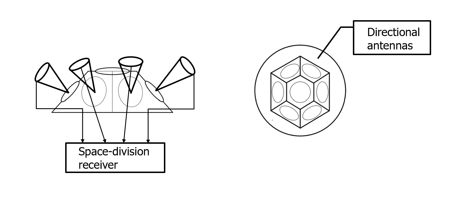
Assume that there are $K$ users and an array with $M$ PMTs as a space division receiver. To make the system model more comprehensible, Fig. 2 shows the planar graph of a space division multiuser uplink system with $K=3$ and $M=9$.

Due to extremely large path loss of NLOS UV link, the received signal can be characterized by discrete photoelectrons whose arrivals satisfy a Poisson random process. Denote the mean number of arrival photons of the signal from user $k$ to PMT $m$ as $\boldsymbol{\lambda_{s}}(k,m)$, and that of background noise of PMT $m$ as $\boldsymbol{\lambda_{n}}(m)$, respectively. Assume that all users are sending OOK modulated signals. Letting $N_{k,m}$ denote the number of received photoelectrons at PMT $m$ from user $k$, we have

where $\eta_{m}$ denotes the quantum efficiency of PMT $m$, $P_{k}$ denotes the emitting power of user $k$, $T_{s}$ denotes the symbol duration, and $\xi_{k,m}$ denotes the path loss from user $k$ to PMT $m$.

The signals from multiple PMTs can be combined to improve the detection performance, expecially under multiuser interference. Assume that $(N_{1},...,N_{M})$ are the photon numbers of $M$ PMTs detected in a symbol slot. In this work, we adopt the following linear combination,

where $\{\alpha_{1},\alpha_{2},...,\alpha_{M}\}$ is the weight vector.

Based on Eq. (2), assuming independent photon arrivals at multiple receiving PMTs, the mean and variance of $W$ are given as follows,

Note that weighted sum $W$ can be approximated via a Gaussian dustributed variable, denoted as $W^{G}\sim{\cal N}(\mathbb{E}(W),\mathbb{VAR}(W))$. The accuracy of such approximation can be validated in Section VI.

In order to select the optimal signal detection method, channel parameters between all the users and receiving PMTs should be accurately estimated. Suppose that $K\times L$ estimation pilot matrix

is adopted for channel estimaiton, which is known to the receiver. It means that each user will send a $L$-symbol length pilot sequence (For example, user $1$ sends $(x_{1,1},x_{1,2},...,x_{1,L})$). Assume that the channel parameters from all users to PMT $m$ are

All the parameters shown in Eq. (8) can be estimated using the detected photon number of PMT $m$ in $L$ symbol durations, denoted as

In fact, each element of $\boldsymbol{u_{m}}$ satisfies Poisson distribution. Noting that the Poisson arrival intensity of each symbol duration is influenced by $K$ users simultaneously, we have that

Similar to [25], an unbiased channel estimator, denoted as $\boldsymbol{\hat{\lambda}_{sr}}(m)$, is given as follows,

and the corresponding estimation MSE is given by,

In the system, all the users’ signals are OOK modulated symbols. Let $\boldsymbol{X}=(\boldsymbol{x}_{1},\boldsymbol{x}_{2},...,\boldsymbol{x}_{L})$, where each $\boldsymbol{x}_{l}$ is a $K\times 1$ colomn vector corresponding to the pilot symbols in slot $l$.

Balanced structure is adopted for the design of pilot matrix $\boldsymbol{X}$, where each user sends with the same frequency in a block. In our design, it’s expected that any $R$ users selected from the whole $K$ users simultaneously appear with the same frequency for any $k=1,2,...,K$. To explain this property more clearly, given matrix $\boldsymbol{X}$ as shown in Eq. (II-B) and an index group $\Theta=\{\theta_{1},...,\theta_{R}\}$, define

Based on Eq. (13), for $\forall\Theta\subseteq\{1,2,...,K\}$ with $\|\Theta\|_{0}=R$ for any $1\leq R\leq K$, it’s expected that $\zeta_{\boldsymbol{X}}(\Theta)$ is only a function of $R$. Matrix $\boldsymbol{X}$ will be considered to be a balanced structure if such a property is satisfied.

Considering $R$, define matrix

where $\boldsymbol{x}_{i}$ is a $K\times 1$ vector and $\|\boldsymbol{x}_{i}\|_{1}=R$ for $1\leq i\leq C^{R}_{K}$. $C^{R}_{K}$ indicates the possible modes given weight $R$. An example is given as follows for $K=4$ and $R=2$,

Based on the above definition, define group $\boldsymbol{\Xi}$ as the set of matrix generated via column concatenation of matrices in $\{\boldsymbol{X}^{(1)},\boldsymbol{X}^{(2)},...,\boldsymbol{X}^{(K)}\}$ with totally $2^{K}-1$ elements. Specifically, we let

We have the following results on all matrices in $\boldsymbol{\Xi}$.

Considering the estimation of $\boldsymbol{\lambda_{sr}}(m)=[\boldsymbol{\lambda_{s}}(1,m),\boldsymbol{\lambda_{s}}(2,m),...,\boldsymbol{\lambda_{s}}(K,m)]$ using the detected photon numbers of PMT $m$. Based on Eq. (12), assuming known background noise intensity $\boldsymbol{\lambda_{n}}(m)$. Denote $\|\boldsymbol{\lambda_{sr}}(m)\|_{1}$ as the element-wise first-order norm of $\boldsymbol{\lambda_{sr}}(m)$ as the channel gain parameters from $K$ users to PMT $m$. Considering pilot matrix $\boldsymbol{X}$ with balanced structure, we have the following preliminary results refer to Theorem 1.

Moreover, based on Eq. (22), if $\boldsymbol{X}=\boldsymbol{X}^{\boldsymbol{\hat{\beta}}}$ for $\boldsymbol{\hat{\beta}}=\{\hat{\beta}_{1},...,\hat{\beta}_{S}\}$, we have

The optimal pilot matrix design for the estimation of $\boldsymbol{\lambda_{sr}}(m)=[\boldsymbol{\lambda_{s}}(1,m),\boldsymbol{\lambda_{s}}(2,m),...,\boldsymbol{\lambda_{s}}(K,m)]$ is formulated by solving the following problem,

Consider two users, user $A$ and user $B$, which are sending OOK modulated signal and each time only one user is allowed to send. We aim to design a detection rule to help the receiver decide which user is more likely to send signals. In this situation, the detection error rate equals the probability that the receiver chooses a wrong user. Assume that the mean photon arrival numbers of desired signal components from user $A$ to the $M$ PMTs are $(\boldsymbol{\lambda_{a}^{s}}(1),...,\boldsymbol{\lambda_{a}^{s}}(M))$, the mean photon arrival numbers of desired signal components from user $B$ to the $M$ PMTs are $(\boldsymbol{\lambda_{b}^{s}}(1),...,\boldsymbol{\lambda_{b}^{s}}(M))$, and the mean photon arrival numbers of background noise of $M$ PMTs are $\boldsymbol{\lambda_{n}}=(\boldsymbol{\lambda_{n}}(1),...,\boldsymbol{\lambda_{n}}(M))$. Denote that,

Assume that the pulse numbers of all the $M$ PMTs corresponding to user $A$ within a symbol duration are $(N_{a,1},...,N_{a,M})$, and those for user $B$ are $(N_{b,1},...,N_{b,M})$. Letting $\{\alpha_{m}\}^{M}_{m=1}$ denote the weights, the weighted sums are given by

Gaussian approximations of $W_{A}$ and $W_{B}$ are introduced, denoted as $W_{A}\sim\mathcal{N}(\mu_{a},\sigma_{a}^{2})$ and $W_{B}\sim\mathcal{N}(\mu_{b},\sigma_{b}^{2})$, respectively. According to Eq. (II-A), we have

Assume prior probability $p(a=1)=p(b=1)=0.5$. Since weight vector $\boldsymbol{\alpha}$ can be adjusted, without loss of generality, assume that $\mu_{a}\geq\mu_{b}$. Then, the detection error pobability with detection threshold $th$, denoted as $p_{e}$, is given by,

Based on Eq. (35), the optimal detection threshold, denoted as $\hat{th}$, is given by

Based on the above threshold, the detection error based on Gaussian approximation is given as follows,

where $Q(\bullet)$ denotes Gaussian Q-function. Let $V(A)=\frac{\mu_{a}-\hat{th}}{\sigma_{a}}$ and $V(B)=\frac{\hat{th}-\mu_{b}}{\sigma_{b}}$. We have the following

Considering the scenario with large $\lambda_{s}$ and $\lambda_{s}/\lambda_{n}$, we have

Since $\sqrt{1+X}\approx 1+\frac{1}{2}X$ when $X\ll 1$, we have

Similar approximation holds for $V(F)$, given by

The detection error can be approximated as follows,

We aim to maximize $\frac{\mu_{a}-\mu_{b}}{\sigma_{a}+\sigma_{b}}$, which can be written as follows according to Eq. (IV-A).

Notice that Eq. (43) is a homogeneous function to $\boldsymbol{\alpha}$. Without loss of generality, with constraint $\|\boldsymbol{\alpha}\|=1$, an optimization problem is proposed,

Due to complicated form of the denominator, maximizing $Div(\boldsymbol{\alpha},\boldsymbol{\lambda_{st}}(a),\boldsymbol{\lambda_{st}}(b))$ is intractable. We resort to maximizing a lower bound. Since

a lower bound on $Div(\boldsymbol{\alpha},\boldsymbol{\lambda_{st}}(a),\boldsymbol{\lambda_{st}}(b))$, denoted as $Div^{LB}(\boldsymbol{\alpha},\boldsymbol{\lambda_{st}}(a),\boldsymbol{\lambda_{st}}(b))$, is given by

The optimization problem can be transformed to maximizing the following lower bound,

Based on Cauchy-Inequality, we have that,

The equality holds if and only if,

and one solution to the optimal weight coefficients is given by

Based on Eq. (36) and Eq. (50), an optimal detection rule aiming to seperate two users can be proposed. Denote an indicator function $I$, if user $A$ is detected, $I=1$, and if user $B$ is detected, $I=0$. Assume that the detected photon numbers are $(N_{1},...,N_{M})$. For certain threshold $\hat{th}$, we have that,

Given the channel parameter vectors of user $A$ and $B$, we can adopt Eq. (42) and Eq. (IV-B) to obtain the minimum detection error probability, denoted as $p_{e}^{th}(A,B)$, given by

Suppose that the received photon numbers of $M$ PMTs are $(N_{1},...,N_{M})$. If ML detection is adopted to two-user seperation problem, the detection rule and the error calculation are shown as follows,

Here we assume $p(a)=p(b)=\frac{1}{2}$. It can be seen that the calculation of $p_{e}^{ML}(A,B)$ is much more complicated than that of $p_{e}^{th}(A,B)$. Moreover, the expression of $p_{e}^{th}(A,B)$ is more tractable, and the simulation results show that $p_{e}^{th}(A,B)$ is pretty close to $p_{e}^{ML}(A,B)$. Thus, we can greatly simplify the performance evaluation procedure while maintaining the optimal behavior through threshold detection.

The analysis of these part is based on Eq. (52). Since there exists inevitable channel estimation errors, we aim to investigate the sensitivity of detection error probability to imperfect channel estimation. Let

while $p_{e}$ can be expressed as follows,

Assume that the estimation bias occurs on $\boldsymbol{\lambda_{a}}(m)$. Then, the absolute value of $\frac{\partial p_{e}}{\partial\boldsymbol{\lambda_{a}}(m)}$, which can characterize the detection sensitivity, is shown as follows,

Denote that $I_{1}=\frac{1}{2\sqrt{2\pi}G_{a,b}}\ exp(-\frac{{G_{a,b}}^{2}}{2})$ and $I_{2}=\bigg|1-\bigg(\frac{2}{1+\frac{\boldsymbol{\lambda_{a}}(m)}{\boldsymbol{\lambda_{b}}(m)}}\bigg)^{2}\bigg|$. Letting $x=\frac{\boldsymbol{\lambda_{a}}(m)}{\boldsymbol{\lambda_{b}}(m)}$, obviously we have $x>0$. Thus, we have,

References

- [1] Z. Xu and B. M. Sadler, “Ultraviolet communications: potential and state-of-the-art,” IEEE Communications Magazine, vol. 46, no. 5, pp. 67–73, 2008.
- [2] H. Elgala, R. Mesleh, and H. Haas, “Indoor optical wireless communication: potential and state-of-the-art,” IEEE Communications Magazine, vol. 49, no. 9, pp. 56–62, 2011.
- [3] H. Ding, G. Chen, A. K. Majumdar, B. M. Sadler, and Z. Xu, “Modeling of non-line-of-sight ultraviolet scattering channels for communication,” IEEE Journal on Selected Areas in Communications, vol. 27, no. 9, pp. 1535–1544, 2009.
- [4] T. Y. Aung, S. Arya, and Y. H. Chung, “Performance dependence of non-line-of-sight ultraviolet communications on atmospheric parameters of the ultraviolet channel,” Optics Communications, vol. 443, pp. 7–11, 2019.
- [5] H. Xiao, Y. Zuo, J. Wu, H. Guo, and J. Lin, “Non-line-of-sight ultraviolet single-scatter propagation model,” Optics Express, vol. 19, no. 18, pp. 17 864–17 875, 2011.
- [6] G. Chen, L. Liao, Z. Li, R. J. Drost, and B. M. Sadler, “Experimental and simulated evaluation of long distance nlos uv communication,” in 2014 9th International Symposium on Communication Systems, Networks & Digital Sign (CSNDSP). IEEE, 2014, pp. 904–909.
- [7] L. Liao, R. J. Drost, Z. Li, T. Lang, B. M. Sadler, and G. Chen, “Long-distance non-line-of-sight ultraviolet communication channel analysis: experimentation and modelling,” IET Optoelectronics, vol. 9, no. 5, pp. 223–231, 2015.
- [8] D. K. Borah, V. R. Mareddy, and D. G. Voelz, “Single and double scattering event analysis for ultraviolet communication channels,” Optics Express, vol. 29, no. 4, pp. 5327–5342, 2021.
- [9] Z. Xu, H. Ding, B. M. Sadler, and G. Chen, “Analytical performance study of solar blind non-line-of-sight ultraviolet short-range communication links,” Optics Letters, vol. 33, no. 16, pp. 1860–1862, 2008.
- [10] L. Wang, Z. Xu, and B. M. Sadler, “Non-line-of-sight ultraviolet link loss in noncoplanar geometry,” Optics Letters, vol. 35, no. 8, pp. 1263–1265, 2010.
- [11] Y. Sun and Y. Zhan, “Closed-form impulse response model of non-line-of-sight single-scatter propagation,” JOSA A, vol. 33, no. 4, pp. 752–757, 2016.
- [12] R. J. Drost, T. J. Moore, and B. M. Sadler, “Ultraviolet scattering propagation modeling: analysis of path loss versus range,” JOSA A, vol. 30, no. 11, pp. 2259–2265, 2013.
- [13] T. Wu, J. Ma, P. Su, R. Yuan, and J. Cheng, “Modeling of short-range ultraviolet communication channel based on spherical coordinate system,” IEEE Communications Letters, vol. 23, no. 2, pp. 242–245, 2019.
- [14] C. Gong, X. Zhang, Z. Xu, and L. Hanzo, “Optical wireless scattering channel estimation for photon-counting and photomultiplier tube receivers,” IEEE Transactions on Communications, vol. 64, no. 11, pp. 4749–4763, 2016.
- [15] D. Zou, C. Gong, K. Wang, and Z. Xu, “Characterization on practical photon counting receiver in optical scattering communication,” IEEE Transactions on Communications, vol. 67, no. 3, pp. 2203–2217, 2018.
- [16] S. M. Haas and J. H. Shapiro, “Capacity of wireless optical communications,” IEEE Journal on Selected Areas in Communications, vol. 21, no. 8, pp. 1346–1357, 2003.
- [17] K. Chakraborty, S. Dey, and M. Franceschetti, “Outage capacity of MIMO Poisson fading channels,” IEEE Transactions on Information Theory, vol. 54, no. 11, pp. 4887–4907, 2008.
- [18] A. Lapidoth and S. Shamai, “The Poisson multiple-access channel,” IEEE Transactions on Information Theory, vol. 44, no. 2, pp. 488–501, 1998.
- [19] G. Wang, C. Gong, and Z. Xu, “Signal characterization for multiple access non-line of sight scattering communication,” IEEE Transactions on Communications, vol. 66, no. 9, pp. 4138–4154, 2018.
- [20] A. Chaaban, Z. Rezki, and M.-S. Alouini, “On the capacity of the intensity-modulation direct-detection optical broadcast channel,” IEEE Transactions on Wireless Communications, vol. 15, no. 5, pp. 3114–3130, 2016.
- [21] A. Chaaban, O. M. S. Al-Ebraheemy, T. Y. Al-Naffouri, and M.-S. Alouini, “Capacity bounds for the Gaussian IM-DD optical multiple-access channel,” IEEE Transactions on Wireless Communications, vol. 16, no. 5, pp. 3328–3340, 2017.
- [22] H. Kim, B. Nachman, and A. El Gamal, “Superposition coding is almost always optimal for the Poisson broadcast channel,” IEEE Transactions on Information Theory, vol. 62, no. 4, pp. 1782–1794, 2016.
- [23] C. Gong, Q. Gao, and Z. Xu, “Signal detection for superposition transmission protocols for optical wireless scattering broadcast channel,” IEEE Transactions on Wireless Communications, vol. 17, no. 8, pp. 5480–5493, 2018.
- [24] A. Sokolovsky and S. I. Bross, “Attainable error exponents for the Poisson broadcast channel with degraded message sets,” IEEE Transactions on Information Theory, vol. 51, no. 1, pp. 364–374, 2005.
- [25] C. Gong and Z. Xu, “Channel estimation and signal detection for optical wireless scattering communication with inter-symbol interference,” IEEE Transactions on Wireless Communications, vol. 14, no. 10, pp. 5326–5337, 2015.
- [26] B. Liu, C. Gong, J. Cheng, and Z. Xu, “Correlation-based LTI channel estimation for multi-wavelength optical scattering NLOS communication,” IEEE Transactions on Communications, vol. 68, no. 3, pp. 1648–1661, 2019.
- [27] B. Liu, C. Gong, J. Cheng, Z. Xu, and J. Liu, “Blind and Semi-Blind channel estimation/equalization for Poisson channels in optical wireless scattering communication systems,” IEEE Transactions on Wireless Communications, vol. 21, no. 8, pp. 5930–5946, 2022.
- [28] N. D. Chatzidiamantis, G. K. Karagiannidis, and M. Uysal, “Generalized maximum-likelihood sequence detection for photon-counting free space optical systems,” IEEE Transactions on Communications, vol. 58, no. 12, pp. 3381–3385, 2010.
- [29] C. Gong and Z. Xu, “LMMSE SIMO receiver for short-range non-line-of-sight scattering communication,” IEEE Transactions on Wireless Communications, vol. 14, no. 10, pp. 5338–5349, 2015.
- [30] C. Gong, K. Wang, Z. Xu, and X. Wang, “On full-duplex relaying for optical wireless scattering communication with on-off keying modulation,” IEEE Transactions on Wireless Communications, vol. 17, no. 4, pp. 2525–2538, 2018.
- [31] M. H. Ardakani, A. R. Heidarpour, and M. Uysal, “Performance analysis of relay-assisted NLOS ultraviolet communications over turbulence channels,” IEEE/OSA Journal of Optical Communications and Networking, vol. 9, no. 1, pp. 109–118, 2017.
- [32] S. Arya and Y. H. Chung, “State-of-the-art ultraviolet multiuser indoor communication over power-constrained discrete-time Poisson channels,” Optical Engineering, vol. 59, no. 10, pp. 106 106–106 106, 2020.
- [33] H. Ge, X. Zhou, Y. Chen, J. Zhang, W. Ni, X. Wang, and L. Zheng, “Shot-noise-limited photon-counting precoding scheme for MIMO ultraviolet communication in atmospheric turbulence,” Optics Express, vol. 31, no. 1, pp. 426–441, 2023.
- [34] X. Zhou, D. Zhang, R. Zhang, and L. Hanzo, “A photon-counting spatial-diversity-and-multiplexing MIMO scheme for Poisson atmospheric channels relying on Q-ary PPM,” Optics Express, vol. 20, no. 24, pp. 26 379–26 393, 2012.
- [35] C. Abou-Rjeily, “Spatial multiplexing for photon-counting MIMO-FSO communication systems,” IEEE Transactions on Wireless Communications, vol. 17, no. 9, pp. 5789–5803, 2018.
- [36] M. L. Riediger, R. Schober, and L. Lampe, “Multiple-symbol detection for photon-counting MIMO free-space optical communications,” IEEE Transactions on Wireless Communications, vol. 7, no. 12, pp. 5369–5379, 2008.
- [37] A. Gupta and M. Brandt-Pearce, “Receiver design for shot noise limited MIMO FSO/UV communication systems,” in 2012 IEEE Globecom Workshops. IEEE, 2012, pp. 1183–1187.