CERN-TH-2023-062

A thermal product formula

Matthew Dodelson^a Cristoforo Iossa^b,c Robin Karlsson^a, and Alexander Zhiboedov^a Affiliation: ^aCERN, Theoretical Physics Department, CH-1211 Geneva 23, Switzerland Affiliation: ^bSISSA, via Bonomea 265, 34136 Trieste, Italy Affiliation: ^cINFN, sezione di Trieste, via Valerio 2, 34127 Trieste, Italy

Abstract

We show that holographic thermal two-sided two-point correlators take the form of a product over quasi-normal modes (QNMs). Due to this fact, the two-point function admits a natural dispersive representation with a positive discontinuity at the location of QNMs. We explore the general constraints on the structure of QNMs that follow from the operator product expansion, the presence of the singularity inside the black hole, and the hydrodynamic expansion of the correlator. We illustrate these constraints through concrete examples. We suggest that the product formula for thermal correlators may hold for more general large $N$ chaotic systems, and we check this hypothesis in several models.

1 Introduction

A thermal two-point function describes the response of a system at finite temperature to a small perturbation kadanoff1963hydrodynamic. In theories with simple holographic duals, it is captured by the wave equation in a black hole background Maldacena:1997re; Gubser:1998bc; Witten:1998qj; Witten:1998zw; Son:2002sd.
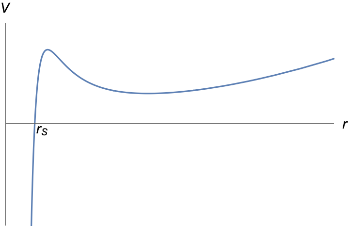
In this paper we mostly (but not only!) concern ourselves with holographic CFTs, for which the relevant geometry is a black hole in AdS. For this case, the problem of computing the thermal response is reduced to a quantum-mechanical scattering problem in a potential $V(z)$ which encodes the black hole geometry. Very generally for non-extremal black holes, this potential has the following features,¹¹ 1 Here $z$ is the tortoise coordinate, i.e. $dz=-{dr\over f(r)}$ , where $f(r)$ is the black hole redshift factor.

\displaystyle V(z)\sim\begin{cases}\frac{1}{z^{2}}&z\to 0\penalty\ \penalty\ \penalty\ \penalty\ \text{(AdS boundary)},\\ \sum_{n=1}^{\infty}a_{n}e^{-\frac{4\pi n}{\beta}z}&z\to\infty\penalty\ \penalty\ \penalty\ \text{(BH horizon)}.\end{cases}

(1)

The exponential decay close to the horizon is consistent with the periodicity of the potential $V(z)=V(z+i{\beta\over 2})$ under complex shifts of $z$ .

Let us denote the two-sided thermal function that can be obtained by solving the wave equation as $G_{12}(\omega)$ , where we keep the angular/spatial momentum dependence implicit. There are two basic facts about $G_{12}(\omega)$ that will be important for us in the present paper:

•

It is a meromorphic function of $\omega$ Hartnoll:2005ju; festucciathesis; Festuccia:2005pi. Its singularities, known as quasi-normal modes (QNMs), encode the characteristic decay of perturbations in time Horowitz:1999jd; Berti:2009kk.
•

It has no zeros, or in other words, ${1\over G_{12}(\omega)}$ is an entire function of $\omega$ . This property is intimately related to the behavior of the potential $V(z)$ close to the black hole horizon, see festucciathesis and Appendix C.

Even though these properties have been extracted by studying classical wave propagation on a black hole background, at the level of the thermal two-point function they can be considered more generally in situations where there is no well-defined notion of a classical geometry or black hole horizon. In fact, extrapolating beyond holography, we will find that both properties hold at finite coupling in several low-dimensional examples of large $N$ systems.

The two properties above imply, modulo simple technical details deferred to the main text, that we can write a product formula representation for the two-sided correlator,²² 2 The condition $G_{12}(0)>0$ is a consequence of unitarity, see Section 2.

\displaystyle G_{12}(\omega)={G_{12}(0)\over\prod_{n=1}^{\infty}(1-{\omega^{2}\over\omega_{n}^{2}})(1-{\omega^{2}\over(\omega_{n}^{*})^{2}})},\penalty\ \penalty\ \penalty\ \penalty\ G_{12}(0)>0.

(2)

In other words, the two-point function is fixed by the QNMs up to an overall rescaling. No further data (such as the residues at the poles) is required. Note that the same statement translates to the retarded two-point function $G_{R}(t)$ for $t>0$ , see Appendices A and B. In frequency space we have the following relation

\displaystyle G_{12}(\omega)=\frac{G_{R}(\omega)-G_{R}(-\omega)}{2i\sinh(\beta\omega/2)},\penalty\ \penalty\ \penalty\ \penalty\ \penalty\ \penalty\ \omega\in\mathbb{C}\ .

(3)

Another characteristic feature of the black hole geometry in $AdS_{d+1>3}/CFT_{d>2}$ is the presence of the curvature singularity. In Festuccia:2005pi it was argued that the singularity leads to exponential decay of the two-sided two-point function at large imaginary $\omega$ . An illuminating way to encode this property is to say that the two-sided correlator obeys the following dispersive sum rules

\displaystyle\text{BH singularity}:\penalty\ \penalty\ \penalty\ \oint_{C_{\infty}}d\omega^{\prime}\,(\omega^{\prime})^{m}G_{12}(\omega^{\prime})=0,

(4)

see Figure 1. Again, even though (4) was extracted by studying the classical wave equation, it is interesting to contemplate the possibility that it holds more generally and consider its violation as some sort of “resolution” of the singularity.

The purpose of this paper is to analyze the general properties of the product formula (13), as well as to explore its workings in various examples. In particular, we study the constraints imposed on the structure of QNMs by the OPE; we discuss how the singularity sum rules (4) are satisfied and violated; and finally, we explore the relation between the structure of QNMs and the low-energy (hydrodynamic) expansion of the correlator. In the latter case, we find that the hydrodynamic expansion encodes certain moments of the QNM density.

After examining the general constraints, we specialize to several analytically solvable examples, including BTZ and Rindler space. We then proceed to discuss several examples in pure GR and beyond for which no analytic expression is available. To compute the QNMs for these cases, we use the package $\mathtt{QNMSpectral}$ Jansen:2017oag.

In the final section of the paper, we show that the two-point functions in several SYK-type models satisfy the holographic properties mentioned above. We conclude by presenting a hypothesis regarding the two-point function in planar chaotic theories, and with a discussion of various open directions.

2 Analytic structure of thermal two-point functions

In this paper we are mainly interested in the two-sided thermal two-point function, defined as follows,

\displaystyle G_{12}(t,\vec{x})\equiv\left\langle{\cal O}\left(t-\frac{i\beta}{2},\vec{x}\right){\cal O}(0,0)\right\rangle_{\beta}={1\over Z(\beta)}{\rm tr}\Big[e^{-\beta H}{\cal O}\left(t-\frac{i\beta}{2},\vec{x}\right){\cal O}(0,0)\Big],

(5)

where $\beta$ is the inverse temperature and the spatial coordinate $\vec{x}$ labels a point on the spatial manifold on which the CFT lives. We will mostly consider the case where $\vec{x}\in\mathbb{R}^{d-1}$ in the present paper.

We will be considering $G_{12}(t,\vec{x})$ in Fourier space

\displaystyle G_{12}(\omega,k)

\displaystyle=\int dt\,d^{d-1}\vec{x}\,e^{i\omega t-i\vec{k}\cdot\vec{x}}G_{12}(t,\vec{x}),\penalty\ \penalty\ \penalty\ \vec{x}\in\mathbb{R}^{d-1},

(6)

where $k\equiv|\vec{k}|$ . We will be mostly concerned with the dependence of the two-sided correlator on $\omega$ , while keeping $k$ fixed. We will therefore sometimes write $G_{12}(\omega)$ with the spatial dependence kept implicit. We have chosen to work with $G_{12}(\omega,k)$ because of its nice properties, but all other two-point functions can be easily obtained once $G_{12}(\omega,k)$ is known, see Appendix A.

2.1 Definitions and general properties

Let us review some basic properties of the two-sided thermal two-point function $G_{12}(\omega)$ as a function of $\omega$ :

•

Unitarity: on the real axis the two-sided correlator is real and non-negative

$\displaystyle G_{12}(\omega)\geq 0,\penalty\ \penalty\ \penalty\ \omega\in\mathbb{R}.$ (7)

This property simply follows from the insertion of a complete set of states between the two operators in the definition of the two-sided correlator and unitarity of the underlying theory.³³ 3 In the most general setting, $G_{12}(\omega)$ is a distribution, and therefore (7) should be understood in the distributional sense. In the present paper we will treat $G_{12}(\omega)$ as a function. In particular, we will study its analytic properties in the complex $\omega$ plane. We believe that this is justified for interacting CFTs on $S^{1}\times\mathbb{R}^{d-1}$ and large $N$ interacting CFTs on $S^{1}\times S^{d-1}$ above the Hawking-Page phase transition Hawking:1982dh. It is true by inspection for holographic CFTs. Assuming that $G_{12}(\omega)$ is real-analytic for real $\omega$ , we get in the complex plane

$\displaystyle G_{12}^{*}(\omega)=G_{12}(\omega^{*}).$ (8)

When $G_{12}(\omega)=0$ on the real axis something special happens, namely the local operator with a given energy $\omega$ annihilates the thermal state. We expect that this is only possible in free (or integrable) theories, and that in interacting theories $G_{12}(\omega)>0$ on the real axis.
•

KMS symmetry: the two-sided correlator is even under $\omega\to-\omega$ ,

$\displaystyle G_{12}(\omega)=G_{12}(-\omega).$ (9)
•

OPE limit: the large frequency limit of the correlator is universal and is controlled by the unit operator,

$\displaystyle\lim_{\omega\to+\infty}G_{12}(\omega)\sim e^{-{\beta\omega\over 2}}\omega^{2\Delta-d},$ (10)

where $\Delta$ is the conformal dimension of $\mathcal{O}$ and the proportionality coefficient is known exactly in terms of $d$ and $\Delta$ . As we will see later, corrections to this formula at large $\omega$ can be systematically computed in the $1/\omega$ expansion, and are determined by the OPE coefficients and thermal one-point functions of operators that appear in the $\mathcal{O}\times\mathcal{O}$ OPE expansion.

The properties above hold in any CFT and do not rely on holography.

2.2 Properties of holographic thermal correlators

Next we list the properties of $G_{12}(\omega)$ which are specific for theories with a classical gravity dual:

•

Meromorphy: the only singularities of $G_{12}(\omega)$ are isolated simple poles in the complex plane Hartnoll:2005ju; festucciathesis; Festuccia:2005pi.⁴⁴ 4 Double poles are allowed on the imaginary axis (although imaginary poles are still generically simple). For instance in $AdS_{3}/CFT_{2}$ there are double poles on the imaginary axis when $k=0$ . These singularities correspond to quasi-normal modes (QNMs), and they characterize the real-time decay of a perturbation to the thermal plasma Horowitz:1999jd; Berti:2009kk. By virtue of (8) and (9), QNMs come in families $(\omega_{n},-\omega_{n},\omega_{n}^{*},-\omega_{n}^{*})$ . Similarly, the residues of $G_{12}(\omega)$ for various frequencies within one family are all related to each other,

\displaystyle\text{Res}_{\omega_{n}}G_{12}(\omega)=-\text{Res}_{-\omega_{n}}G_{12}(\omega)=(\text{Res}_{\omega_{n}^{*}}G_{12}(\omega))^{*}=-(\text{Res}_{-\omega_{n}^{*}}G_{12}(\omega))^{*}.

(11)

•

No zeros: the two-sided correlator does not have zeros in the complex $\omega$ -plane festucciathesis. This property follows from the fact that the two-sided correlator is obtained by solving the wave equation in the black hole background and from the universal properties of the scattering potential close to the black hole horizon, see Appendix C. Put differently, $1/G_{12}(\omega)$ is an entire function.

•

Asymptotic behavior: along any ray in the complex plane that asymptotically avoids poles, the two-sided correlator satisfies

\displaystyle\left|\frac{1}{G_{12}(\omega)}\right|\sim e^{\lambda(\theta)r},\hskip 14.22636pt\omega=re^{i\theta}\to\infty,\hskip 14.22636pt\lambda(\theta)\geq 0,

(12)

up to a polynomial prefactor. In other words, $1/G_{12}(\omega)$ is an entire function of order one. The asymptotic behavior (12) follows from the large $\omega$ expansion of the wave equation, see festucciathesis.

The three properties above imply the following product formula for holographic thermal correlators⁵⁵ 5 An analogous product formula appeared in the context of thermal functional determinants Denef:2009kn, but for thermal correlators we are not aware of such results in the literature.,

\displaystyle G_{12}(\omega)={G_{12}(0)\over\prod_{n=1}^{\infty}(1-{\omega^{2}\over\omega_{n}^{2}})(1-{\omega^{2}\over(\omega_{n}^{*})^{2}})}.

(13)

To see this, we use Hadamard’s factorization theorem, see e.g. conway2012functions, which states that an entire function $f(z)$ of order $m$ and zeroes $a_{n}$ can be written as

\displaystyle f(z)=z^{\ell}e^{P(z)}\prod_{n=1}^{\infty}E_{\left\lfloor m\right\rfloor}(z/a_{n}),

(14)

where $P(z)$ is a polynomial of degree $q\leq m$ and

\displaystyle E_{\left\lfloor m\right\rfloor}(z)=(1-z)\prod_{k=1}^{\left\lfloor m\right\rfloor}e^{z^{k}/k}

(15)

are elementary factors. By assumption, $1/G_{12}$ is of order $m=1$ . Imposing evenness, $\ell=0$ , and noting that $E_{1}(z)E_{1}(-z)=E_{0}(z)E_{0}(-z)=1-z^{2}$ , the product formula follows.

In writing (13) we assumed that $\omega^{*}_{n}\neq-\omega_{n}$ , which is not true for purely imaginary QNMs. It is trivial to extend the ansatz by including the product of purely imaginary simple modes $\omega_{n}=i\tilde{\omega}_{n}$ as follows, $\prod_{n=1}^{\infty}\left(1+{\omega^{2}\over\tilde{\omega}_{n}^{2}}\right)^{-1}$ .

2.3 Black hole singularity sum rules

In Festuccia:2005pi; festucciathesis it was shown that for the Schwarzschild black hole, $G_{12}(\omega)$ at large imaginary $\omega$ is controlled by a real geodesic that bounces off the black hole singularity Kraus:2002iv; Fidkowski:2003nf. As a result, the correlator decays exponentially as $\omega\to\pm i\infty$ Festuccia:2005pi; festucciathesis,

\displaystyle|G_{12}(\omega)|\sim e^{-\tilde{\beta}|\omega|/2},\hskip 28.45274pt\omega\to\pm i\infty,\hskip 28.45274pt\tilde{\beta}=\beta\cot\left(\frac{\pi}{d}\right).

(16)

The two-point function is also exponentially decaying in the region $\omega\to\pm\infty$ , where it is controlled by the OPE behavior (10). Therefore in the presence of the curvature singularity there exists a positive number $\kappa$ such that (avoiding the poles)

\displaystyle\frac{|G_{12}(\omega)|}{e^{-\kappa|\omega|}}\to 0\text{ as }|\omega|\to\infty,\hskip 28.45274pt\kappa>0.

(17)

This is a stronger condition than (12), which allows for a vanishing decay rate $\lambda(\theta)=0$ along some complex ray.
We can use the condition (17) to write down a simple set of sum rules,⁶⁶ 6 By singularity here we mean the curvature singularity. For example, (18) does not hold for the BTZ black hole.

Figure 1: The contour integral along

C_{\infty}

in (18) vanishes due to the asymptotic decay of the correlator. By deforming the integration contour inside and picking up the contribution of QNMs we get the sum rules (19).

\displaystyle\text{BH singularity}:\penalty\ \penalty\ \penalty\ \oint_{C_{\infty}}d\omega^{\prime}\,(\omega^{\prime})^{m}G_{12}(\omega^{\prime})=0,

(18)

see Figure 1. The asymptotic behavior (17) guarantees that the contour integrals (18) vanish. We can then deform the contour and rewrite these sum rules in terms of the residues of $G_{12}(\omega)$ , $\lambda_{n}$ , at the QNMs $\omega=\omega_{n}$ . For $m$ even the sum vanishes identically, but for $m$ odd we find a nontrivial constraint:

\displaystyle\text{Re}\sum_{n}\omega_{n}^{m}\lambda_{n}=0,\hskip 28.45274pt\text{ for odd }m>0,

(19)

where we used the relations (11) between residues of poles in the same family. Note that the sum rules (19) immediately imply that the residues $\lambda_{n}$ decay exponentially fast in $n$ . As we will see in Section 5.3, the singularity sum rules follow directly from the product formula (13) with some mild assumptions on the asymptotic structure of QNMs. In Section 5.3 we will use the exponential decay at $\omega\to i\infty$ along with the OPE to uniquely fix the leading high-energy asymptotics of QNMs.

Let us also notice that we can consider finite energy singularity sum rules by placing the integration contour $C_{\Lambda}$ in (18) at some finite radius $|\omega|=\Lambda$ .⁷⁷ 7 See e.g. Dolen:1967jr; Mukhametzhanov:2018zja; Noumi:2022wwf for discussions of finite energy sum rules in the context of scattering amplitudes. In particular, in Mukhametzhanov:2018zja they were rigorously derived using Tauberian theorems. In this case the sum rules are satisfied up to exponentially small corrections $e^{-c\Lambda}$ . The advantage of considering sum rules at finite $\omega$ is that we expect them to hold also at finite ’t Hooft coupling (or string length) as long as $\Lambda\lesssim{1\over l_{s}}$ .

3 QNMs and black hole geometry

In the next section we will analyze various constraints placed on the QNMs by the product formula (13). To set the stage for these constraints, let us first give a brief overview of QNMs and their connection to the geometry of the black hole background, closely following Festuccia:2008zx; festucciathesis. For a detailed review, see Berti:2009kk.
We consider a spherically symmetric asymptotically $AdS_{d+1}$ black hole, with metric

\displaystyle ds^{2}=-f(r)\,dt^{2}+\frac{dr^{2}}{f(r)}+r^{2}\,d\Omega_{d-1}^{2}.

(20)

In order to write the scalar field wave equation $(\Box-\Delta(\Delta-d))\phi=0$ in a convenient form, let us Fourier expand

\displaystyle\phi(t,\vec{x},r)=e^{-i\omega t}Y_{J\vec{m}}(\Omega)r^{-(d-1)/2}\psi(\omega,J,r),

(21)

where $Y_{J\vec{m}}$ are spherical harmonics on $S^{d-1}$ . In terms of $\psi$ , the wave equation takes the form of the Schrodinger equation for a particle in a potential,

(-\partial_{z}^{2}+V(J,z)-\omega^{2})\psi=0,

(22)

where $dz=-\frac{dr}{f(r)}$ is the tortoise coordinate. The horizon is located at $z=\infty$ and the boundary at $z=0$ . The potential is given by

\displaystyle V(J,z)=f(r)\left(\frac{J(J+d-2)}{r^{2}}+\nu^{2}-\frac{d^{2}}{4}+\frac{(d-1)f^{\prime}(r)}{2r}+\frac{(d-1)(d-3)}{4r^{2}}f(r)\right),

(23)

where $\nu=\Delta-d/2$ . The potential for a black brane takes the same form, with $J(J+d-2)$ replaced with $k^{2}$ .
Now let us discuss the behavior of the potential (23) near the horizon and infinity. For a general AdS black hole, the asymptotic behavior is universally given by

V(J,z)\sim\begin{cases}\frac{\nu^{2}-\frac{1}{4}}{z^{2}}&z\to 0\\ \sum_{n=1}^{\infty}a_{n}(J)e^{-\frac{4\pi n}{\beta}z}&z\to\infty.\end{cases}

(24)

The behavior at the boundary follows from the asymptotics $f(r)\sim r^{2}$ at large $r$ . The structure of the potential near the horizon can be justified as follows. Since the redshift factor $f(r)$ has a simple zero at the horizon $r_{S}$ , we can expand

\displaystyle f(r)=\frac{4\pi}{\beta}(r-r_{S})+\sum_{n=2}^{\infty}\frac{1}{n!}\frac{d^{n}f}{dr^{n}}(r_{S})(r-r_{S})^{n}.

(25)

The tortoise coordinate is then

	$\displaystyle z$	$\displaystyle=z_{0}-\int^{r}dr\,\left(\frac{\beta}{4\pi(r-r_{s})}-\frac{\beta^{2}f^{\prime\prime}(r_{S})}{32\pi^{2}}+\ldots\right)$		(26)
		$\displaystyle=z_{0}-\frac{\beta}{4\pi}\log(r-r_{S})+\frac{\beta^{2}}{32\pi^{2}}f^{\prime\prime}(r_{S})(r-r_{S})+\ldots$		(27)

Solving for $r(z)$ , we find

\displaystyle r=r_{S}+\exp\left(-\frac{4\pi}{\beta}(z-z_{0})\right)+\frac{\beta}{8\pi}f^{\prime\prime}(r_{S})\exp\left(-\frac{8\pi}{\beta}(z-z_{0})\right)+\ldots,

(28)

where the higher corrections are of the form $\exp\left(-4\pi n(z-z_{0})/\beta\right)$ . Since the potential is an analytic function of $r$ , we therefore find that the potential takes the form shown in (24).
Because perturbations can fall into the horizon, we cannot define normal modes of the scalar field. Instead, we consider quasi-normal modes, which are ingoing at the horizon and normalizable at the boundary,

	$\displaystyle\psi(z)$	$\displaystyle\sim e^{i\omega z},\hskip 28.45274ptz\to\infty$		(29)
	$\displaystyle\psi(z)$	$\displaystyle\sim z^{\frac{1}{2}+\nu},\hskip 28.45274ptz\to 0.$		(30)

Such resonances can only exist at a discrete set of complex energies, which satisfy $\text{Im }\omega<0$ for real $J$ Horowitz:1999jd. Note that $\text{Im }\omega<0$ implies that perturbations decay in time, whereas poles in the upper half plane would lead to a growing mode, signifying an instability of the black hole. There are also constraints on QNMs from causality Brigante:2007nu; Brigante:2008gz; Heller:2022ejw, but we do not explore them in this paper.
In order to obtain a qualitative understanding of the structure of QNMs, it is useful to consider the WKB limit $\Delta\to\infty$ with $\omega/\Delta$ and $J/\Delta$ fixed. The potential (23) then takes the form

\displaystyle V(z)=f(r)\left(\frac{J^{2}}{r^{2}}+\Delta^{2}\right).

(31)

For $z_{0}$ extremizing the potential, there exists a line of QNM poles emanating from $\sqrt{V(z_{0})}$ . However, not all extrema contribute. To find the relevant values of $z_{0}$ , one must first solve the equation $V(r)=u^{2}$ for the turning point $r(u)$ . The physical turning point is defined to be the solution $r(u)$ which behaves as $r(u)\sim u/\Delta$ for large real $u$ . Then the extrema of the potential corresponding to QNMs are those at which the physical turning point merges with another turning point at some value of $u$ in the lower half plane. We refer the reader to Festuccia:2008zx for further details.

The first few modes of this line of poles are given by the expression

\displaystyle\omega_{n}=\sqrt{V(z_{0})}+\left(n+\frac{1}{2}\right)\sqrt{\frac{V^{\prime\prime}(z_{0})}{2V(z_{0})}},\hskip 28.45274ptn=0,1,\ldots

(32)

The branches of the square roots should be chosen so that $\omega_{n}$ is in the lower half plane.
Let us now discuss several important cases of the Bohr-Sommerfeld approximation to QNMs.

•

Weakly damped modes: The first example we consider is where $V(z)$ has a metastable minimum outside the horizon, as depicted in Figure 2(a). Then in the approximation (32), the associated QNMs are purely real. The imaginary part is exponentially small since it is related to tunneling over the potential barrier, and it is not captured by the leading WKB approximation. Since these modes decay very slowly, they represent the leading contribution to the two-point function at late times. One case where such a metastable minimum arises is at large $J$ . The corresponding modes are related to stable orbits around the black hole Festuccia:2008zx; festucciathesis; Dodelson:2022eiz; Gannot:2012pb; Berenstein:2020vlp.
•

Virtual bound states: In the previous example, the minimum of the potential was outside the horizon. We can also consider the case where the minimum is behind the horizon in a region where $V(z_{0})<0$ , see Figure 2(b). We see from (32) that the modes are then purely imaginary. Charged black holes provide an example of this phenomenon, as we will see later. In this case, there is a stable minimum of the potential between the inner and outer horizon.
•

Complex extrema: Generically, extrema of the potential are at some arbitrary point in the complex plane off the real $r$ axis. In this case there is no clean physical interpretation of the QNMs in terms of the real section of the geometry. Note that the extrema come in complex conjugate pairs, since $V^{*}(r)=V(r^{*})$ . Therefore a complex extremum leads to two lines of poles related by $\omega_{n}\to-\omega_{n}^{*}$ , at an angle determined by (32). For example, consider the QNMs of the black brane metric $f(r)=r^{2}-1/r^{d-2}$ at zero spatial momentum. There are $d$ complex extrema at $r^{d}=1-d/2$ , but the only two that contribute according to the prescription described above have phase $e^{\pm i\pi/d}$ . This leads to two lines of poles in the lower half plane at angles $e^{-\pi i/d}$ and $e^{-(d-1)\pi i/d}$ Festuccia:2008zx.

Let us now comment on the QNMs beyond the lowest lying modes (32). In the case of a metastable minimum, the low-lying QNMs have exponentially small imaginary part, but at some $n_{\text{max}}$ the modes go off into the complex plane at a finite angle. Therefore there are only finitely many weakly damped modes. In contrast, the virtual bound states and modes associated to complex extrema go on forever. As we will see later, there must be infinitely many QNMs in order to reproduce the operator product expansion.
In this section we have discussed the QNMs in the large $\Delta$ limit. The highly damped QNMs can also be computed for order one $\Delta$ by solving the wave equation near the singularity and near the boundary and then matching the two solutions. See Natario:2004jd; Cardoso:2004up for details.

4 Asymptotic Minkowski OPE

Let us consider a CFT two-point function of scalar primary operators on $S^{1}_{\beta}\times\mathbb{R}^{d-1}$ . We can write the following OPE expansion,

\displaystyle\langle{\cal O}(\tau,\vec{x}){\cal O}(0,0)\rangle_{\beta}=\sum_{{\cal O}_{\Delta,J}}{a_{\Delta,J}\over\beta^{\Delta}}C_{J}^{({d-2\over 2})}\Big({\tau\over\sqrt{\tau^{2}+\vec{x}^{2}}}\Big)(\tau^{2}+|\vec{x}|^{2})^{{\Delta-2\Delta_{{\cal O}}\over 2}},

(33)

where $C_{J}^{({d-2\over 2})}(\cos\theta)$ are the usual Gegenbauer polynomials and $\tau$ is the Euclidean time $\beta>\tau\geq 0$ . The sum goes over the primary operators that appear in the OPE of ${\cal O}\times{\cal O}$ , and the expansion coefficients $a_{\Delta,J}$ are given by the product of the corresponding three-point function and thermal expectation value $\langle{\cal O}_{\Delta,J}\rangle_{\beta}$ , see Iliesiu:2018fao for details.

In this paper we are interested in the Lorentzian correlator. More precisely, we consider the two-sided correlator, which is related to the Euclidean correlator above as follows,

\displaystyle G_{12}(\omega,k)

\displaystyle=\int_{-\infty}^{\infty}dt\,e^{i\omega t}\left\langle{\cal O}\left({\beta\over 2}+it,\vec{k}\right){\cal O}(0,0)\right\rangle_{\beta}\ .

(34)

We would like to understand how the OPE expansion (33) constrains the form of $G_{12}(\omega,k)$ . We will be interested in the limit $\omega\beta\gg 1$ with

\displaystyle\zeta\equiv{k\over\omega}\geq 0

(35)

kept fixed.

It has been suggested in Caron-Huot:2009ypo that in this limit the two-sided correlator admits the following asymptotic Minkowski OPE expansion

\displaystyle G_{12}(\omega,k)

\displaystyle=e^{-{\beta\omega\over 2}}\omega^{2\Delta_{{\cal O}}-d}\theta(1-\zeta)\sum_{{\cal O}_{\Delta,J}}{a_{\Delta,J}\over(\beta\omega)^{\Delta}}G_{\Delta,J}(\zeta)+O(e^{-\beta\omega}),

(36)

where the conformal blocks $G_{\Delta,J}(\zeta)$ take the following form (see Appendix D for the derivation),

	$\displaystyle G_{\Delta,J}(\zeta)$	$\displaystyle=\frac{\pi^{\frac{d}{2}+1}2^{d+\Delta-2\Delta_{{\cal O}}+1}\Gamma(d+J-2)}{\Gamma(d-2)\Gamma(J+1)\Gamma\left(\frac{J}{2}-\frac{\Delta}{2}+\Delta_{{\cal O}}\right)\Gamma\left(-\frac{d}{2}-\frac{J}{2}-\frac{\Delta}{2}+\Delta_{{\cal O}}+1\right)}{}$
		$\displaystyle\times\left(1-\zeta^{2}\right)^{\frac{1}{2}(2\Delta_{{\cal O}}-d-\Delta-J)}\ _{2}F_{1}\left({1-J\over 2},-{J\over 2},{d-1\over 2},\zeta^{2}\right).$		(37)

The support of $G_{12}(\omega,k)$ in (36), namely the presence of $\theta(1-\zeta)$ , was discussed in Manenti:2019wxs. This expansion is supported by the known holographic and perturbative examples and we will assume it to be true in this paper. Note that $G_{12}(\omega,k)$ is nonzero for $k>\omega$ , but it is expected to be exponentially suppressed in this region Son:2002sd; Papadodimas:2012aq; Banerjee:2019kjh.

The basic idea behind (36) is the following. The coordinate space OPE leads to the large frequency expansion of the Euclidean correlator. The behavior of the Euclidean correlator at large Matsubara frequencies controls the behavior of the retarded correlator via the relation $G_{E}(\omega_{n})=G_{R}(i\omega_{n})$ . Consider next the subtracted dispersion relation for the retarded correlator. The large frequency behavior at imaginary frequencies controls the large behavior of the spectral density or, equivalently, the two-sided correlator via complex Tauberian theorems for the Stieltjes transform Mukhametzhanov:2018zja. Assuming that the $G_{12}(\omega,k)$ itself admits a power-like expansion leads to the formulas above. More generally, rigorous formulas can be derived as in Mukhametzhanov:2018zja. This is particularly relevant for finite $c_{T}$ CFTs on a sphere, where $G_{12}(\omega)$ is given by a sum of $\delta$ -functions.

We next discuss the universal contribution to the OPE as well as its structure in holographic theories.

4.1 The unit operator and the stress tensor

The leading contribution at large frequencies comes from the unit operator $\Delta=J=0$ . The first subleading correction comes from the stress tensor. The leading terms in the expansion of the two-point function thus take the following form

	$\displaystyle{G_{12}(\omega,k)\over e^{-{\beta\omega\over 2}}\omega^{2\Delta_{{\cal O}}-d}}$	$\displaystyle\stackrel{{\scriptstyle 1+T}}{{=}}{4^{{d+1\over 2}-\Delta_{{\cal O}}}\pi^{{d\over 2}+1}(1-\zeta^{2})^{\Delta_{{\cal O}}-d/2}\over\Gamma(\Delta_{\cal O})\Gamma(\Delta_{\cal O}+1-{d\over 2})}{}$
		$\displaystyle+{a_{T}\over(\beta\omega)^{d}}{4^{d-\Delta_{{\cal O}}}(d-1)(d-2)\pi^{{d\over 2}+1}\over\Gamma(\Delta_{\cal O}-d)\Gamma(\Delta_{\cal O}+1-{d\over 2})}(1-\zeta^{2})^{\Delta_{{\cal O}}-d}\Big(1+{d\over d-1}{\zeta^{2}\over 1-\zeta^{2}}\Big),$		(38)

where the coefficient of the stress tensor is fixed by the Ward identities as follows,

\displaystyle a_{T}=-fS_{d}{2\Delta_{\cal O}\over d-2}{c_{\text{free}}\over c_{T}}.

(39)

Here $S_{d}=\text{vol}(S^{d-1})={2\pi^{d/2}\over\Gamma(d/2)}$ and $c_{\text{free}}={d\over d-1}{1\over S_{d}^{2}}$ is the free boson two-point function of the stress tensor. Finally, $f$ is related to the free energy density as follows

\displaystyle f\equiv{F\over T^{d}}.

(40)

For holographic theories a convenient formula was found in Kovtun:2008kw

\displaystyle f_{\text{holo}}=-\frac{2^{2d-3}(d-1)\left(\frac{1}{d}\right)^{d+1}\pi^{d/2}\Gamma\left(d/2\right)^{3}}{(d+1)\Gamma(d)}S_{d}^{2}c_{T},

(41)

where we used that $f=-{s\over d}$ , and $s$ is the entropy density. Plugging this into (39) we get

\displaystyle a_{T}^{\text{holo}}=\frac{2^{d-2}\left(\frac{1}{d}\right)^{d}\pi^{d+\frac{1}{2}}\Gamma\left(\frac{d}{2}-1\right)}{\Gamma\left(\frac{d+3}{2}\right)}\Delta_{\cal O}.

(42)

We have tested this formula in the case of an AdS black brane by numerically solving the wave equation at large $\omega$ . Let us also notice that for $\Delta_{\cal O}=d,d-1,...$ , the contribution of the stress tensor drops out.

4.2 Multi-stress tensor operators

Next we discuss the contribution of multi-stress tensor operators $T^{n}$ to the OPE. These have scaling dimension $\Delta_{T^{n}}=nd$ and spin $0\leq J\leq 2n$ . In a generic CFT it is not known how to compute the contribution of these operators to the OPE.

For theories with gravity duals it can be done, see Fitzpatrick:2019zqz. Indeed, their contribution is controlled by the physics close to the AdS boundary. To keep the discussion simple, let us present the result for the contribution of $T^{2}$ operators in $d=4$ . Combining the results above with the ones in Fitzpatrick:2019zqz we get⁸⁸ 8 We set in Fitzpatrick:2019zqz $f_{0}=(\pi/\beta)^{4}$ , which is valid for the black brane.

$\displaystyle{G_{12}^{\text{holo}}(\omega,k)\over e^{-{\beta\omega\over 2}}\omega^{2\Delta_{{\cal O}}-4}}$	$\displaystyle\stackrel{{\scriptstyle T^{2}}}{{=}}{1\over(\omega\beta)^{8}}\frac{\pi^{11}4^{3-\Delta_{{\cal O}}}\Delta_{{\cal O}}\left(1-\zeta^{2}\right)^{\Delta_{{\cal O}}-8}}{1575\Gamma(\Delta_{{\cal O}}-5)\Gamma(\Delta_{{\cal O}}-1)}(c_{0}+c_{2}\zeta^{2}+c_{4}\zeta^{4})$	(43)
$\displaystyle c_{0}$	$\displaystyle=7\Big(9\Delta_{{\cal O}}^{4}-95\Delta_{{\cal O}}^{3}+240\Delta_{{\cal O}}^{2}+80\Delta_{{\cal O}}+96\Big)\ ,{}$
$\displaystyle c_{2}$	$\displaystyle=6\Big(7\Delta_{{\cal O}}^{4}-105\Delta_{{\cal O}}^{3}+280\Delta_{{\cal O}}^{2}+400\Delta_{{\cal O}}+288\Big)\ ,{}$
$\displaystyle c_{4}$	$\displaystyle=7\Delta_{{\cal O}}^{4}-65\Delta_{{\cal O}}^{3}+160\Delta_{{\cal O}}^{2}+240\Delta_{{\cal O}}+288\ .{}$

Notice that the effect that we observed at the level of a single stress tensor, namely vanishing of its contribution for $\Delta_{{\cal O}}=3$ and $\Delta_{{\cal O}}=4$ , continues here as well. We see that for $\Delta_{{\cal O}}=3,4,5$ the expression above vanishes.

We believe the same effect continues for $T^{n}$ , and therefore we can write simple closed form expressions (up to nonperturbative corrections) for the OPE expansion. It follows that (4.1) represents the full answer for $\Delta_{{\cal O}}=3,4,5$ in $d=4$ .

4.3 Leading nonperturbative correction

We now consider the leading nonperturbative correction to the large frequency expansion above. In coordinate space this correction has a regular expansion at small separations and therefore we expect that it could be related to the double trace operators. These are operators schematically of the form $\mathcal{O}\Box^{n}\partial^{\mu_{1}}\partial^{\mu_{2}}\dots\partial^{\mu_{J}}\mathcal{O}$ . In the limit we are working their scaling dimension is $2\Delta_{\mathcal{O}}+J+2n$ . Therefore, we see from (33) that they will contribute to the OPE with analytic terms.

For theories with gravity duals these corrections can be computed by analyzing the wave equation in the large $\omega$ regime, see festucciathesis and references therein. The solution to the wave equation close to both the singularity and the boundary can be approximated by Bessel functions in the tortoise coordinate $z$ . For large $\omega$ the regions of validity of these approximations overlap and it is possible to obtain a solution valid for all $z$ . Finally, one can use such a solution to extract the leading order contribution to (36) with its nonperturbative corrections (but no power law corrections). The leading term with the first nonperturbative correction reads

\displaystyle G_{12}^{\text{holo}}\left(\omega,0\right)\simeq e^{-\frac{\beta\omega}{2}}\omega^{2\Delta_{\mathcal{O}}-d}{4^{{d+1\over 2}-\Delta_{\mathcal{O}}}\pi^{{d\over 2}+1}\over\Gamma\left(\Delta_{\mathcal{O}}\right)\Gamma\left(\Delta_{\mathcal{O}}+1-{d\over 2}\right)}\left(1-4e^{-{\beta\omega\over 2}}\cos\left(\pi\left(\Delta_{\mathcal{O}}-{d\over 2}\right)-{\tilde{\beta}\omega\over 2}\right)\right)\,.

(44)

In Appendix E we show that this correction can be reproduced from the exact expression for $G_{12}(\omega,0)$ found in Dodelson:2022yvn.

5 QNMs and the OPE

We have argued that the quasi-normal modes determine the holographic Wightman function up to a constant. By providing additional input for $G_{12}$ , we can place constraints on the spectrum of QNMs.

In this section, we will input the constraint from the operator product expansion at large real frequency. As $\omega\to+\infty$ , we should recover the zero temperature answer up to an overall factor of $e^{-\beta\omega/2}$ , see Katz:2014rla; Caron-Huot:2009kyg; Manenti:2019wxs,

\displaystyle G_{12}(\omega)\sim\omega^{2\Delta-d}e^{-\beta\omega/2},\hskip 28.45274pt\omega\to+\infty,

(45)

where the proportionality constant and subleading in ${1\over\omega}$ corrections can be found in the previous section.

The goal is to use this constraint to derive conditions on the asymptotic behavior of QNMs. The first step is to convert the product over QNMs into a convenient sum. From (13), we have

\displaystyle\partial_{\omega}\log G_{12}(\omega)=-\sum_{n}\left(\frac{1}{\omega-\omega_{n}}+\frac{1}{\omega+\omega_{n}}+\frac{1}{\omega-\omega_{n}^{*}}+\frac{1}{\omega+\omega_{n}^{*}}\right).

(46)

On the other hand, from (45) we have

\displaystyle\partial_{\omega}\log G_{12}(\omega)\sim-\frac{\beta}{2}+\frac{2\Delta-d}{\omega}+\ldots

(47)

Let us now compare these two expressions. It is immediately clear that (47) implies that the number of QNMs has to be infinite and that they must extend all the way to infinity. Indeed, imagine that there are a finite number of QNMs. Then $\partial_{\omega}\log G_{12}(\omega)\sim{1\over\omega}$ at large $\omega$ , which is not consistent with (47).

Next we consider several simple ways in which QNMs can approach infinity and see how this approach is constrained by the OPE.

5.1 A single line of asymptotic QNMs

Figure 3: A single line of evenly spaced QNMs with angle

\theta

and spacing

r

We start with the simplest case, where the QNMs are asymptotically organized into a single line at angle $\theta$ , see Figure 3. We consider the following ansatz⁹⁹ 9 Strictly speaking these are the images of QNMs under KMS symmetry, not QNMs themselves.

\displaystyle\omega_{n}=re^{i\theta}n^{\alpha}+\ldots,\hskip 28.45274ptn\gg 1,\penalty\ \penalty\ \penalty\ 0<\theta<\pi/2.

(48)

Computing the large $\omega$ behavior of the sum we get

	$\displaystyle\partial_{\omega}\log G_{12}(\omega)$	$\displaystyle=-\sum_{n=1}^{\infty}\left(\frac{1}{\omega-re^{i\theta}n^{\alpha}}+\text{images}\right)$
		$\displaystyle\approx-\frac{2\pi}{\alpha\omega}\left(\frac{\omega}{r}\right)^{1/\alpha}\frac{\cos\left(\frac{\pi-2\theta}{2\alpha}\right)}{\sin\left(\frac{\pi}{2\alpha}\right)},$		(49)

where the leading asymptotic does not depend on the lower limit in the sum.

Matching to the leading term in (47), we find

\displaystyle\alpha=1

(50)

and

\displaystyle\beta=\frac{4\pi\sin\theta}{r}.

(51)

For a line of simple poles on the imaginary axis, one should divide the right hand side of (51) by two, since there is only one image.
Let us now consider the first subleading term at large $n$ . For this purpose, we take the improved ansatz

\displaystyle\omega_{n}=re^{i\theta}n+se^{i\phi}+\ldots\ .

(52)

Using the Euler-Maclaurin formula, the sum (46) to order $1/\omega$ is

$\displaystyle\partial_{\omega}\log G_{12}(\omega)$	$\displaystyle\approx-\frac{1}{2}\left(\frac{1}{\omega-\omega_{1}}+\text{images}\right)-\frac{2\pi\sin\theta}{r}+\frac{4}{\omega}{}$
	$\displaystyle\hskip 14.22636pt-\int_{1}^{\infty}dn\,\left(\frac{se^{i\phi}}{(\omega-re^{i\theta}n)^{2}}+\text{images}\right)$
	$\displaystyle\approx-\frac{2\pi\sin\theta}{r}+\frac{4s\cos(\theta-\phi)+2r}{r\omega}.$	(53)

Comparing with (47), we find

\displaystyle 2\Delta-d=\frac{4s\cos(\theta-\phi)+2r}{r}.

(54)

To shed more light on this result, let us imagine that we add an extra QNM at $\omega_{0}$ . A single QNM contributes at large $\omega$ as $\partial_{\omega}\log G_{12}(\omega)\sim-{4\over\omega}$ . For the computation above adding a single QNM corresponds to effectively relabeling $n\to n-1$ , which shifts the subleading constant as $se^{i\phi}\to se^{i\phi}-re^{i\theta}$ . Plugging this expression into (53) indeed leads to the expected shift $-{4\over\omega}$ . In this sense the subleading term in (52) is sensitive to the global structure of QNMs, but it is not sensitive to the details of their distributions at low energies.

To summarize, we have learned that for a single line of QNMs, the spectrum must be asymptotically linearly spaced. Moreover, the spacing and angle must be related in terms of the temperature, and the first subleading term in the expansion is related to the conformal dimension of the operator under consideration. These conditions apply for any black hole solution in which there is only one line of asymptotic QNMs. For example, the QNMs of massless fields with $\Delta=d$ in large $AdS_{d+1}$ /Schwarzschild black holes asymptotically approach the line¹⁰¹⁰ 10 In flat space a similar formula was first derived in Motl:2003cd. Cardoso:2004up; Natario:2004jd

\displaystyle\omega_{n}\simeq\frac{4\pi}{\beta}\sin\left(\frac{\pi}{d}\right)e^{i\pi/d}\left(n+\frac{d-2}{4}-i\frac{\log 2}{2\pi}\right)+...\ ,

(55)

which is easily seen to satisfy (51) and (54). Notice that the OPE expansion effectively maps to the ${1\over n}$ expansion of the QNMs. Moreover, we see that at each order in the expansion we have two real parameters to fix, and we have only one equation.
To proceed to subleading orders we can write

\displaystyle\omega_{n}=re^{i\theta}n+se^{i\phi}+\frac{te^{i\psi}}{n^{\gamma}}+\ldots\hskip 28.45274pt\gamma>0.

(56)

If $\gamma$ is an integer, then it is straightforward to check that subleading terms in $\partial_{\omega}\log G_{12}(\omega)$ receive contributions from all $n$ in the sum, so we cannot fix $t$ purely in terms of the asymptotics of the QNMs. Let us now consider the case where $\gamma$ is fractional. At large $\omega$ , the sum (46) is dominated by $n\sim\omega$ , so we can expand the summand in $n^{-\gamma}$ . Expanding $\partial_{\omega}\log G_{12}$ at large $\omega$ and plugging in (54) and (51) gives

	$\displaystyle\partial_{\omega}\log G_{12}(\omega)$	$\displaystyle\approx-\frac{\beta}{2}+\frac{2\Delta-d}{\omega}-\int_{1}^{\infty}dn\,\left(\frac{te^{i\psi}n^{-\gamma}}{(\omega-re^{i\theta}n)^{2}}+\text{images}\right)$
		$\displaystyle\approx-\frac{\beta}{2}+\frac{2\Delta-d}{\omega}+\frac{2\pi t\gamma r^{\gamma-1}\cos\left(\theta-\psi+\gamma\left(\frac{\pi}{2}-\theta\right)\right)}{\omega^{\gamma+1}\sin\left(\frac{\pi\gamma}{2}\right)}.$		(57)

Since fractional powers of $\omega$ do not appear in the OPE expansion of $\partial_{\omega}\log G_{12}(\omega)$ for holographic correlators, it must be the case that

\displaystyle\psi=\pm\frac{\pi}{2}+\theta+\gamma\left(\frac{\pi}{2}-\theta\right).

(58)

In Section 6, we will check this relation for AdS black branes.
We have seen that fractional powers can appear in the expansion of the QNMs at subleading orders. In fact, if there are two asymptotic lines of QNMs, fractional powers can appear in the leading behavior of one of the lines. We turn to this case next.

5.2 Adding another asymptotic line

Figure 4: The ansatz (61) and (62) for

\alpha=2

. The red points are evenly spaced, and the blue points scale quadratically with

n

We now consider the case of several asymptotic lines of poles. If all the lines are asymptotically linearly spaced, then the previous calculation generalizes immediately, and we find

\displaystyle\beta=4\pi\sum_{i}\frac{\sin\theta_{i}}{r_{i}}.

(59)

As mentioned above, a line of simple imaginary poles needs to be treated separately, and contributes $2\pi/r_{i}$ to this sum. Similarly, we have the subleading constraint

\displaystyle 2\Delta-d=\sum_{i}\frac{4s_{i}\cos(\theta_{i}-\phi_{i})+2r_{i}}{r_{i}}\ .

(60)

The more interesting situation is when not all lines are asymptotically linearly spaced. Let us consider the case of two asymptotic lines. We take one of the lines along the imaginary axis for simplicity, and choose the ansatz

	$\displaystyle\omega_{1,n}$	$\displaystyle=ian^{\alpha}+\ldots,\hskip 28.45274ptn\gg 1,\penalty\ a>0,\penalty\ \alpha>1$		(61)
	$\displaystyle\omega_{2,n}$	$\displaystyle=re^{i\theta}n+se^{i\phi}n^{\gamma}+\ldots,\hskip 28.45274ptn\gg 1,\penalty\ 0<\theta<\pi/2,\penalty\ 0<\gamma<1.$		(62)

Proceeding as above, we find

$\displaystyle\partial_{\omega}\log G_{12}(\omega)$	$\displaystyle\approx-\int_{1}^{\infty}dn\,\left[\left(\frac{1}{\omega-ian^{\alpha}}+\text{image}\right)+\left(\frac{1}{\omega-re^{i\theta}n}+\text{images}\right)\right.$
	$\displaystyle\hskip 85.35826pt\left.-\left(\frac{e^{i\phi}n^{\gamma}s}{(\omega-e^{i\theta}nr)^{2}}+\text{images}\right)\right]$	(63)
	$\displaystyle\approx-\frac{2\pi\sin\theta}{r}-\frac{\pi}{\alpha\omega}\left(\frac{\omega}{a}\right)^{1/\alpha}\frac{1}{\sin\left(\frac{\pi}{2\alpha}\right)}+\frac{2\pi s\gamma}{\omega r}\left(\frac{\omega}{r}\right)^{\gamma}\frac{\cos\left(\phi-\theta+\gamma\left(\frac{\pi}{2}-\theta\right)\right)}{\sin\left(\frac{\pi\gamma}{2}\right)}.$

We now match powers of $\omega$ to the OPE expansion (47). The first term in (5.2) reproduces the result (51) from before. The other terms must cancel, giving the conditions $\gamma=1/\alpha$ and

\displaystyle s=r\left(\frac{r}{a}\right)^{1/\alpha}\frac{1}{2\cos\left(\phi-\theta+\frac{1}{\alpha}(\pi/2-\theta)\right)}.

(64)

We will confirm this prediction later by analyzing the QNMs in the presence of a higher derivative correction $W^{2}\phi^{2}$ , where $W$ is the Weyl tensor. This higher derivative term introduces a new line of QNMs on the imaginary axis with asymptotic $n^{3}$ scaling, and we will see numerically that (64) is satisfied to high accuracy in this case.

5.3 Behavior in the complex $\omega$ plane

So far, we have analyzed the behavior of the correlator at large real $\omega$ . Let us now discuss what happens when $\omega$ is taken to infinity along some complex ray. In the case of a single line of QNMs, the lines of poles divide the complex plane into four asymptotic regions. For example, as $\omega\to i\infty$ with the ansatz (48) with $\alpha=1$ , we find

\displaystyle\partial_{\omega}\log G_{12}(\omega)\approx\frac{2\pi i\cos\theta}{r},\hskip 28.45274pt\omega\to i\infty.

(65)

It follows that the correlator exponentially decays at $\omega=i\infty$ with rate $2\pi\cos\theta/r$ . As long as $\theta\not=\pi/2$ , this decay rate is nonzero. Similar remarks apply for the other three regions of the complex plane, so the singularity sum rules (19) are satisfied when $\theta\not=\pi/2$ . We conclude that meromorphy and no zeroes imply the singularity sum rules, given a line of asymptotic QNMs that is not parallel to the imaginary axis.
In fact, the same conclusion holds if there are several lines of asymptotic QNMs, as long as at least one line is at angle $\theta\not=\pi/2$ . The lines divide the complex $\omega$ plane into different asymptotic regions, and in each region the correlator exponentially decays. Therefore the singularity sum rules will be satisfied.

It is instructive to compare the large frequency expansions along the real and imaginary axis. To this end we consider the ratio

\displaystyle\log{G_{12}(\omega)\over G_{12}(i\omega)}={\tilde{\beta}-\beta\over 2}\omega+C_{0}+...\hskip 28.45274pt\beta\omega\gg 1,

(66)

where we wrote only the leading contribution to the ratio and we defined $\tilde{\beta}$ through the leading asymptotic of $\log G_{12}(i\omega)\simeq-{\tilde{\beta}\omega\over 2}$ . Both $\tilde{\beta}$ and $C_{0}$ are sensitive only to the large $n$ tails of the large QNM expansion, and therefore can be safely computed using the same methods that we used above.

Using $\omega_{n}=re^{i\theta}n+se^{i\phi}$ we get

\displaystyle\log{G_{12}(\omega)\over G_{12}(i\omega)}={\beta\over 2}(\cot\theta-1)\omega+\pi\left(\Delta-{d+2\over 2}\right)\tan(\theta-\phi)\ .

(67)

The holographic computation in the AdS-Schwarzschild background gives Festuccia:2005pi; festucciathesis

	$\displaystyle\tilde{\beta}$	$\displaystyle=\beta\cot{\pi\over d},\penalty\ \penalty\ \penalty\ {}$
	$\displaystyle C_{0}$	$\displaystyle=\log 2\ ,$		(68)

which leads to the following expression for the asymptotic behavior of the QNMs,

\displaystyle\omega_{n}\simeq\frac{4\pi}{\beta}\sin\left(\frac{\pi}{d}\right)e^{i\pi/d}\left(n+{\Delta\over 2}-\frac{d+2}{4}-i\frac{\log 2}{2\pi}\right).

(69)

For $\Delta=4$ this agrees with (55).

6 OPE sum rules

In the previous section we explored the basic relationship between the leading terms in the OPE expansion of the correlator and the structure of the QNMs. In this section we show how inputting more data about the asymptotic expansion for the quasi-normal modes leads to exact sum rules for QNMs. These sum rules encode the subleading terms in the OPE expansion, going beyond the previous section.

6.1 OPE sum rules for QNMs

Let us imagine that we have worked out the asymptotic expansion of the QNMs as above to a certain order in ${1\over n}$ , such that

\displaystyle\omega_{n}=\omega_{n}^{\text{asy}}+\delta\omega_{n},

(70)

such that

\displaystyle\lim_{n\to\infty}n^{k_{*}}\delta\omega_{n}=0.

(71)

We can then use the OPE to write down a set of sum rules for $\delta\omega_{n}$ . More precisely, we write

\displaystyle\partial_{\omega}\log G_{12}(\omega)-\partial_{\omega}\log G_{12}^{\text{asy}}(\omega)

\displaystyle=-\sum_{n}\left(\frac{1}{\omega-\omega_{n}^{\text{asy}}-\delta\omega_{n}}-\frac{1}{\omega-\omega_{n}^{\text{asy}}}+\text{images}\right),

(72)

where $G_{12}^{\text{asy}}(\omega)$ is obtained by replacing $\omega_{n}$ with $\omega_{n}^{\text{asy}}$ in the product formula (13) without the prefactor $G_{12}(0)$ . Given the OPE and $\omega_{n}^{\text{asy}}$ we can compute the large $\omega$ expansion of the left hand side. Expanding the right hand side at large $\omega$ under the sum we get

\displaystyle\partial_{\omega}\log G_{12}(\omega)-\partial_{\omega}\log G_{12}^{\text{asy}}(\omega)

\displaystyle=-\sum_{k=1}^{\infty}{4\over\omega^{2k+1}}\sum_{n=1}^{\infty}{\rm Re}\Big((\delta\omega_{n}+\omega_{n}^{\text{asy}})^{2k}-(\omega_{n}^{\text{asy}})^{2k}\Big)\ .

(73)

Such an expansion only makes sense if the sums over $n$ converge. The most dangerous contribution comes from $\delta\omega_{n}(\omega_{n}^{\text{asy}})^{2k-1}\sim\delta\omega_{n}n^{2k-1}$ . For this to converge we require

\displaystyle k_{*}\geq 2k.

(74)

For example, to write down the sum rule corresponding to the contribution of the stress tensor in $d=4$ we need $k=2$ , which requires $k_{*}=4$ .

Let us write more explicitly the first sum rule. We set

\displaystyle\omega_{n}^{\text{asy}}\simeq\frac{4\pi}{\beta}\sin\left(\frac{\pi}{d}\right)e^{i\pi/d}\left(n+{\Delta\over 2}-\frac{d+2}{4}-i\frac{\log 2}{2\pi}\right)-{c\over n^{{d\over d-1}}}e^{i{(d-2)\pi\over 2d(d-1)}},

(75)

where $c$ is computed in Appendix F. Note that the phase of the last term in this expression agrees with the prediction (58).

Using (75), we can write down the first nontrivial sum rule for $k=1$ . The left hand side of (73) takes the form

\displaystyle\partial_{\omega}\log G_{12}(\omega)-\partial_{\omega}\log G_{12}^{\text{asy}}(\omega)=-{\delta c_{3}\over\omega^{3}},

(76)

where $\delta c_{3}$ is given explicitly in (F). Therefore we see that by combining the asymptotic large $n$ expansion of the QNMs with the asymptotic OPE expansion we get exact nonperturbative QNM sum rules, which are sensitive to all QNMs.

Example: $\Delta=4$ , $d=4$

Let us consider the $k=1$ sum rule explicitly for $\Delta=4$ and $d=4$ . Setting $\beta=1$ , we get the following equation

\displaystyle\sum_{n=1}^{\infty}{\rm Re}\Big(\omega_{n}^{2}-(\omega_{n}^{\text{asy}})^{2}\Big)={\delta c_{3}\over 4}\simeq 15.281.

(77)

To check this sum rule let us introduce partial sums $s_{m}\equiv 1-{\sum_{n=1}^{m}{\rm Re}\Big(\omega_{n}^{2}-(\omega_{n}^{\text{asy}})^{2}\Big)\over 15.281}$ . For $m\to\infty$ , the partial sums $s_{m}$ approach 0. We can compute the first few QNMs numerically using $\mathtt{QNMSpectral}$ and check how well the sum rules are satisfied. The reader can find these modes in the accompanying file modes.txt. We plot $s_{m}$ in Figure 5.

Figure 5: We plot the

k=1

OPE sum rule partial sums

s_{m}

for

\Delta=d=4

as a function of

m

We also checked numerically that the leading large $n$ asymptotic of $\delta\omega_{n}$ in this case takes the form $\simeq 0.340{e^{-i{\pi\over 48}}\over n^{7/3}}$ and this tail correctly accounts for the $\sim 23\%$ of the sum rule left for the $k>60$ modes in Figure 5.

6.2 Overall constant

There is one last piece of data that comes from the OPE that we have not used. It is the overall normalization of the correlator at large $\omega$ , as given by (4.1). Similarly, on the product formula side (13), $G_{12}(0)$ has not entered in any of the equations above because it does not contribute to $\partial_{\omega}\log G_{12}(\omega)$ . Likewise, it canceled in the ratio $G_{12}(\omega)/G_{12}(i\omega)$ .

As above, we can imagine that the asymptotic large $n$ expansion of QNMs is known. We then can write

\displaystyle\log G_{12}(\omega)-\log G_{12}^{\text{asy}}(\omega)

\displaystyle=\log G_{12}(0)+\sum_{n=1}^{\infty}\log{(1-{\omega^{2}\over(\omega_{n}^{\text{asy}})^{2}})(1-{\omega^{2}\over(\omega_{n}^{\text{asy}*})^{2}})\over(1-{\omega^{2}\over\omega_{n}^{2}})(1-{\omega^{2}\over(\omega_{n}^{*})^{2}})}.

(78)

We can now take the large $\omega$ limit to get the following equation

\displaystyle\log G_{12}(0)=\log G_{12}^{\text{OPE}}+2\sum_{n=1}^{\infty}\log{|\omega_{n}^{\text{asy}}|^{2}\over|\omega_{n}|^{2}},

(79)

where $\log G_{12}^{\text{OPE}}$ can be computed given the normalization of the vacuum two-point function of the operator of interest and the explicit form of $\omega_{n}^{\text{asy}}$ via the following formula

\displaystyle\log G_{12}^{\text{OPE}}=\lim_{\omega\to\infty}\Big(\log G_{12}(\omega)-\log G_{12}^{\text{asy}}(\omega)\Big).

(80)

Example: shear viscosity in ${\cal N}=4$ SYM at strong coupling

Let us consider the scalar two-point function for $\Delta=4$ in $d=4$ . As reviewed in Appendix G, this is related to the shear viscosity in ${\cal N}=4$ SYM at strong coupling. Setting $d=4$ in (222), the prediction from gravity is

\displaystyle\log G_{12}(0)=\log{\pi^{5}\over 12}\simeq 3.23874,

(81)

where we set $\beta=1$ . We would now like to understand how this result is reproduced from the sum rule (79). The asymptotic form of the QNMs takes the form

\displaystyle\omega_{n}^{\text{asy}}=2\pi(1+i)\left(n+{1\over 2}-i{\log 2\over 2\pi}\right),

(82)

see (75) for $d=4$ . Computing the large $\omega$ limit and using (4.1) we get

\displaystyle\log G_{12}^{\text{OPE}}=\log{\pi^{3}\over 96}-\log\frac{9}{4\sqrt{2}\left(\pi^{2}+\log^{2}(2)\right)^{2}}\simeq 3.07947.

(83)

Therefore we get the following sum rule

\displaystyle\sum_{n=1}^{\infty}\log{|\omega_{n}^{\text{asy}}|^{2}\over|\omega_{n}|^{2}}=\frac{1}{2}\log\left(\frac{9\sqrt{2}\pi^{2}}{\left(\pi^{2}+\log^{2}(2)\right)^{2}}\right)\simeq 0.079637.

(84)

To see how the sum rule is satisfied let us introduce partial sums $s_{m}\equiv 1-{\sum_{n=1}^{m}\log{|\omega_{n}^{\text{asy}}|^{2}\over|\omega_{n}|^{2}}\over 0.079637}$ , so that $\lim_{m\to\infty}s_{m}=0$ . We compute $\omega_{n}$ numerically using $\mathtt{QNMSpectral}$ , and we plot $s_{m}$ in Figure 6.

In principle we can repeat the same computation as above by including the next term in the large $n$ expansion,

\displaystyle\delta\omega_{n}^{\text{asy}}=6\pi\frac{2^{1/6}3^{5/6}e^{-\frac{11i\pi}{12}}\Gamma\left(\frac{5}{6}\right)}{7n^{4/3}\Gamma\left(\frac{1}{6}\right)\Gamma\left(\frac{1}{3}\right)}.

(85)

With this correction the sum rule becomes

\displaystyle\sum_{n=1}^{\infty}\log{|\omega_{n}^{\text{asy}}+\delta\omega_{n}^{\text{asy}}|^{2}\over|\omega_{n}|^{2}}\simeq-0.03873.

(86)

We can again construct partial sums $s_{m}\equiv 1-{\sum_{n=1}^{m}\log{|\omega_{n}^{\text{asy}}+\delta\omega_{n}^{\text{asy}}|^{2}\over|\omega_{n}|^{2}}\over-0.03873}$ , and we plot $s_{m}$ in Figure 6.

Figure 6: We plot the partial sums

s_{m}

for shear viscosity as a function of

m

. The black dots correspond to the choice (82) for the asymptotic modes, whereas the magenta dots include one extra correction as in (85). We see that for the corrected model (in magenta), knowing the first 10 QNMs allows us to satisfy the sum rule with

0.3\%

error.

7 Positive moments for hydrodynamics

It is interesting to see how the location of QNMs translates into the low-energy (hydrodynamic) expansion of the correlator. In this section, we find that by restricting the location of QNMs to a subregion of the complex plane, we get nontrivial bounds on the hydrodynamic expansion coefficients.

The basic observation is that the no-zero property of the thermal correlator can be thought as positivity of the discontinuity of $\log G_{12}(\omega)$ . The product formula (13) corresponds to the dispersive representation of $\log G_{12}(\omega)$ , with $\log G_{12}(0)$ being the subtraction constant. We then find that the coefficients of the low-energy expansion of the two-sided correlator are related to certain moments of the non-negative density of QNMs.

The mathematical structure that emerges is similar to bounds that appear in the context of scattering amplitudes Adams:2006sv. The role of Wilson coefficients is played by the hydrodynamic expansion, whereas the role of dispersion relations is played by the product formula (13).

To follow this idea, it is convenient to introduce a positive-definite measure

	$\displaystyle\rho(\omega)$	$\displaystyle=\sum_{n=1}^{\infty}\delta^{(2)}(\omega-\omega_{n})\ ,{}$
	$\displaystyle\tilde{\rho}(\omega)$	$\displaystyle=\sum_{n=1}^{\infty}\delta(\omega-\tilde{\omega}_{n})\ ,$		(87)

where $\omega_{n}$ are QNMs which satisfy $\text{Re }\omega_{n}>0$ , $\text{Im }\omega_{n}>0$ . As before it is also convenient to separately consider purely imaginary QNMs, for which $\omega=i\tilde{\omega}_{n}$ for real $\tilde{\omega}_{n}$ . In terms of these densities we can write

	$\displaystyle\log{G_{12}(\omega)\over G_{12}(0)}$	$\displaystyle=-\int d^{2}\hat{\omega}\,\rho(\hat{\omega})\log\left[\left(1-{\omega^{2}\over\hat{\omega}^{2}}\right)\left(1-{\omega^{2}\over(\hat{\omega}^{*})^{2}}\right)\right]$
		$\displaystyle\hskip 14.22636pt-\int d\tilde{\omega}\,\tilde{\rho}(\tilde{\omega})\log\left(1+{\omega^{2}\over\tilde{\omega}^{2}}\right).$		(88)

Let us consider next the low energy expansion of the two-sided correlator. It takes the following form,

\displaystyle\log{G_{12}(\omega)\over G_{12}(0)}=\sum_{k=1}^{\infty}(-1)^{k}{2\mu_{k}+\tilde{\mu}_{k}\over k}\omega^{2k},

(89)

where

	$\displaystyle\mu_{k}$	$\displaystyle=\int d^{2}\hat{\omega}\,\rho(\hat{\omega}){\rm Re}{1\over(-i\hat{\omega})^{2k}}\ ,{}$
	$\displaystyle\tilde{\mu}_{k}$	$\displaystyle=\int d\tilde{\omega}\,\tilde{\rho}(\tilde{\omega}){1\over\tilde{\omega}^{2k}}\ .$		(90)

We immediately see that the hydrodynamic expansion is naturally organized in powers of the smallest QNM. To this end, let us introduce $\omega_{\min}$ and $\tilde{\omega}_{\min}$ for the QNMs closest to the origin. It is convenient to define the moments in units of $|\omega_{\text{min}}|$ . For this purpose we can write

\displaystyle\log{G_{12}(\omega)\over G_{12}(0)}=\sum_{k=1}^{\infty}{(-1)^{k}\over k}\left(2\mu_{k}{\omega^{2k}\over|\omega_{\min}|^{2k}}+\tilde{\mu}_{k}{\omega^{2k}\over\tilde{\omega}_{\min}^{2k}}\right),

(91)

where the moments have been defined as follows,

	$\displaystyle\mu_{k}$	$\displaystyle=\int_{\|\hat{\omega}\|\geq 1}d^{2}\hat{\omega}\,\rho(\hat{\omega}){\rm Re}{1\over(-i\hat{\omega})^{2k}}\ ,{}$
	$\displaystyle\tilde{\mu}_{k}$	$\displaystyle=\int_{1}^{\infty}d\tilde{\omega}\,\tilde{\rho}(\tilde{\omega}){1\over\tilde{\omega}^{2k}}\ .$		(92)

We therefore see that the low-energy expansion is related to moments of the QNM density. In fact, the moment problem for $\tilde{\mu}_{k}$ is nothing but the simplest Hausdorff moment problem, which can be seen by switching to $\tilde{y}={1\over\tilde{\omega}^{2}}\in[0,1]$ .

The moment problem for $\mu_{k}$ is more nontrivial since it involves the geometry of the 2d plane. Below we restrict our considerations to the cases where the QNMs are supported in the region $\text{Re }\omega_{n}\leq\text{Im }\omega_{n}$ . For this configuration $\mu_{1}\geq 0$ and it is natural to consider bounds on the ratios $({\mu_{2}\over\mu_{1}},{\mu_{3}\over\mu_{1}})$ . We have derived the bounds in two steps. First, we derived the bounds numerically by discretizing the region of support of QNMs and then solving the coupling maximization problem using $\mathtt{LinearProgramming}$ in Mathematica. We then have identified the boundary of the allowed regions analytically, finding that for the cases considered here they are very simple.

(a)

(b)

Figure 7: (a) We plot the allowed region for the ratios

({\tilde{\mu}_{2}\over\tilde{\mu}_{1}},{\tilde{\mu}_{3}\over\tilde{\mu}_{1}})

of the first three low-frequency expansion coefficients for the case when all QNMs are purely imaginary, see (7.1). The boundary of the allowed region can be realized with two QNMs and one QNM. The red curve corresponds to the zero momentum BTZ correlator (94) as

\Delta

is varied. For small

\Delta\to 0

the moments reach the upper-right cusp. The black and magenta dots are the results for the SYK chain at different momenta for the couplings

v=0.8

and

v=0.2

correspondingly, with the momentum chosen in a range where all the poles are on the imaginary axis. As the momentum becomes small the points approach the the tip of the allowed region. (b) The same plot but zoomed closer to the tip of the allowed region. We see that for small momenta the SYK chain results are close to saturating the upper bound.

7.1 Purely imaginary QNMs

We first consider the simplest case when QNMs are purely imaginary so that $\mu_{i}=0$ . Restricting our attention to $(\tilde{\mu}_{1},\tilde{\mu}_{2},\tilde{\mu}_{3})$ , we can write down a set of optimal constraints Bellazzini:2020cot:

	$\displaystyle\tilde{\mu}_{1}\geq\tilde{\mu}_{2}\geq\tilde{\mu}_{3}\geq 0,{}$
	$\displaystyle\tilde{\mu}_{1}\tilde{\mu}_{3}-(\tilde{\mu}_{2})^{2}\geq 0.$		(93)

The allowed region is depicted in Figure 7.

An example of this type is provided by the BTZ correlator at zero momentum, for which we have

\displaystyle\tilde{\mu}_{1}

\displaystyle={\Delta^{2}\over 2}\psi^{(1)}\left({\Delta\over 2}\right),\penalty\ \penalty\ \penalty\ \tilde{\mu}_{2}={\Delta^{4}\over 48}\psi^{(3)}\left({\Delta\over 2}\right),\penalty\ \penalty\ \penalty\ \tilde{\mu}_{3}={\Delta^{6}\over 3840}\psi^{(5)}\left({\Delta\over 2}\right)\ .

(94)

Doing a shift $\Delta\to\Delta-{d-2\over 2}$ one recovers the Rindler space correlator, and by replacing $\Delta\to{2\over q}$ we get the result in the SYK model.

Let us quickly comment on the structure of the boundary of the allowed region in Figure 7. Let us introduce $0\leq x={1\over\tilde{\omega}}\leq 1$ . Then the green upper line corresponds to $\tilde{\rho}(x)=\alpha\delta(x)+(1-\alpha)\delta(1-x)$ with $0\leq\alpha\leq 1$ , with the upper cusp corresponding to $\alpha=0$ and the lower cusp corresponding to $\alpha=1$ . The blue boundary corresponds to $\rho(x)=\delta(x-x_{0})$ .

(a)

(b)

Figure 8: (a) We plot the allowed region for the ratios

({\mu_{2}\over\mu_{1}},{\mu_{3}\over\mu_{1}})

of the first three low-frequency expansion coefficients for the case when all QNMs lie on the line (95) with

\phi={\pi\over 4}

and

\theta={\pi\over 2}

. The boundary of the allowed region can be realized with two QNMs and one QNM. The red curve corresponds to the

k=\Delta

momentum BTZ correlator (94) as

\Delta

is varied. For small

\Delta\to 0

the moments approach

{\mu_{2}\over\mu_{1}}\to-\infty

and

{\mu_{3}\over\mu_{1}}\to 0

. (b) The same plot but zoomed closer to the boundary of the allowed region. Notice that slightly positive values of

{\mu_{2}\over\mu_{1}}

are realized for certain

\Delta

7.2 QNMs on a line

For the next model we consider the case where all QNMs are located on a single line in the complex plane. In other words, we consider

\displaystyle\omega_{n}=e^{i\phi}+a_{n}e^{i\theta},

(95)

where $a_{n}\geq 0$ and real. This case again effectively reduces to a one-dimensional moment problem. This time, however, it is not easily treated analytically. It is nevertheless straightforward to work out the desired bounds numerically, by reformulating it as a linear programming problem.

To be concrete let us consider the particular case $\phi={\pi\over 4}$ and $\theta={\pi\over 2}$ . We first notice that in this case $\mu_{1}\geq 0$ , where $\mu_{1}=0$ corresponds to a degenerate case where we have a single QNM at $a=0$ , where $a$ is defined in (95). We can then derive the bounds for $({\mu_{2}\over\mu_{1}},{\mu_{3}\over\mu_{1}})$ shown in Figure 8 .

Let us compare the derived bounds with the explicit results for the BTZ black hole for momentum $k=\Delta$ (which corresponds to $\phi={\pi\over 4}$ )

$\displaystyle\mu_{1}$	$\displaystyle={\Delta^{2}\over 4}\left[\psi^{(1)}\left({1+i\over 2}\Delta\right)+\psi^{(1)}\left({1-i\over 2}\Delta\right)\right],{}$
$\displaystyle\mu_{2}$	$\displaystyle={\Delta^{4}\over 48}\left[\psi^{(3)}\left({1+i\over 2}\Delta\right)+\psi^{(3)}\left({1-i\over 2}\Delta\right)\right],{}$
$\displaystyle\mu_{3}$	$\displaystyle={\Delta^{6}\over 1920}\left[\psi^{(5)}\left({1+i\over 2}\Delta\right)+\psi^{(5)}\left({1-i\over 2}\Delta\right)\right]\ .$	(96)

We see that we get a two-sided bound for ${\mu_{3}\over\mu_{1}}$ , but only a one-sided bound for ${\mu_{2}\over\mu_{1}}$ . Moreover, the simplest example of the BTZ black hole correlator realizes arbitrarily negative ${\mu_{2}\over\mu_{1}}$ .

Figure 9: The allowed region for the ratios

({\mu_{2}\over\mu_{1}},{\mu_{3}\over\mu_{1}})

for the case when all QNMs lie in the sectorial domain (97). The boundary of the allowed region can be realized with two QNMs and one QNM. The pink domain corresponds to the BTZ black hole for

0\leq k\leq\Delta

and arbitrary

\Delta

. The black dots represent the results for charged AdS black holes for

\Delta=4

and different values of charge

Q

ranging from

.42

1.27

. In this range the QNMs are all contained within the sectorial region (97).

Let us explain the structure of the boundary of the allowed region in Figure 8. The green upper line corresponds to a pair of QNMs $\rho(a)=\alpha\delta(a-{\sqrt{7}+1\over\sqrt{2}})+(1-\alpha)\delta(a)$ , where $0\leq\alpha\leq 1$ . As $\alpha\to 0$ the point moves to minus infinity, whereas for $\alpha=1$ it touches the blue boundary which is described by a single QNM $\rho(a)=\delta(a-a_{0})$ with $0\leq a_{0}\leq{\sqrt{7}+1\over\sqrt{2}}$ .

7.3 Sectorial QNMs

Finally, we consider the case where the allowed region of support of QNMs is given by a sectorial region:

\displaystyle\text{Im }\omega_{n}\geq 1,\penalty\ \penalty\ \penalty\ \text{Re }\omega_{n}\leq\text{Im }\omega_{n}.

(97)

It includes the two cases considered above but also allows for two-dimensional configurations of QNMs (not necessarily located on a line). We plot the results in Figure 9.

Let us comment on the structure of the boundary in Figure 9. The upper green line corresponds to a pair of QNMs $\rho(\omega)=\alpha\delta(\omega-i)+(1-\alpha)\delta(\omega-(1+i))$ with $0\leq\alpha\leq 1$ . As $\alpha\to 0$ the point on the curve moves to the left, while $\alpha\to 1$ corresponds to the cusp at $(1,1)$ , where we have only one QNM at $i$ . The blue segment corresponds to a single QNM at $\omega_{0}+i$ , where $0\leq\omega_{0}\leq\sqrt{7}-2$ . Finally, the lower green line is described by a pair of QNMs $\rho(\omega)=\alpha\delta(\omega-(\sqrt{7}-2+i))+(1-\alpha)\delta(\omega-(1+i))$ for $0\leq\alpha\leq 1$ .

An obvious question is: what happens to the bounds as we relax the condition (97)? For example, a natural minimal condition to consider is $\text{Im }\omega_{n}\geq 1$ which simply corresponds to the statement that there is a minimal characteristic timescale for perturbations to decay. We have not explored thoroughly what can be said about the structure of the hydrodynamic expansion in this case. However, we observed that for $({\mu_{2}\over\mu_{1}},{\mu_{3}\over\mu_{1}})$ we do not get any nontrivial bounds in this case.

8 BTZ and Rindler space

Next we would like to discuss how the general structure discussed in the previous sections is realized in various examples. We start by considering the simplest examples in which the correlator is known analytically.

The two-sided correlator in the BTZ background is given by Son:2002sd (here $\beta=2\pi$ )

\displaystyle G_{12}(\omega,k)

\displaystyle=\frac{1}{\pi\Gamma(\Delta-1)^{2}}\Gamma\left(\frac{\Delta\pm i(\omega+k)}{2}\right)\Gamma\left(\frac{\Delta\pm i(\omega-k)}{2}\right),

(98)

where $\Gamma(a\pm b)=\Gamma(a+b)\Gamma(a-b)$ . The poles are located at $\omega_{n}=k+i(2n-2+\Delta)$ for $n=1,2,\ldots$ and the three images $(-\omega_{n},\omega_{n}^{*},-\omega_{n}^{*})$ , with residues

\displaystyle\lambda_{n}=\frac{2i(-1)^{n}\Gamma(ik-n+1)\Gamma(n-1+\Delta)\Gamma(-ik+n+\Delta-1)}{\pi(n-1)!\Gamma(\Delta-1)^{2}}.

(99)

The pole spacing is $r=2$ at angle $\theta=\pi/2$ , and the subleading constant correction is $se^{i\phi}=k+(\Delta-2)i$ , so the OPE constraints (51) and (54) indeed hold. Note that the singularity sum rules (19) are not satisfied, since there is no curvature singularity in the BTZ black hole. For instance, truncating the first sum rule at $n=n_{\text{max}}$ gives

\displaystyle\text{Re}\sum_{n=1}^{n_{\text{max}}}\omega_{n}\lambda_{n}\sim-\frac{2k}{\sinh(\pi k)\Gamma(\Delta-1)^{2}}n_{\text{max}}^{2\Delta-1},\hskip 28.45274ptn_{\text{max}}\to\infty

(100)

This diverges as $n_{\text{max}}\to\infty$ , reflecting the fact that the contour integral along $C_{\infty}$ does not vanish.
It is straightforward to verify that the BTZ two-sided correlator (98) can equivalently be written using the product formula (13) with $\omega_{n}=k+i(2n+\Delta)$ (note that $G_{12}(0,k)\neq 1$ in (98), so that the product formula will differ from (98) by a normalization). For $k=0$ the simple poles merge into double poles on the imaginary axis.

An example of known higher-dimensional thermal correlators comes from CFTs on $S^{1}_{\beta}\times\mathbb{H}^{d-1}$ with $\beta=2\pi$ which can be conformally mapped to a Rindler wedge in $\mathbb{R}^{d}$ , see e.g. Casini:2011kv. The scalar two-point function on $S^{1}_{\beta}\times\mathbb{H}^{d-1}$ was studied in Ohya:2016gto and is given by ( $\beta=2\pi$ )

	$\displaystyle G_{12}(\omega,k)$	$\displaystyle=\frac{\pi^{\frac{d-2}{2}}}{\Gamma(\Delta)\Gamma(\Delta-\frac{d-2}{2})}$		(101)
	$\displaystyle\times$	$\displaystyle\Gamma\left(\frac{\Delta-(d-2)/2\pm i(\omega+k)}{2}\right)\Gamma\left(\frac{\Delta-(d-2)/2\pm i(\omega-k)}{2}\right),$		(102)

which reduces to the scalar correlator in BTZ (98) for $d=2$ . Here $k$ labels the principal series representation of $SO(1,d-1)$ , see Ohya:2016gto for details. This has no zeroes, and has poles at $\omega=k+i\left(-\frac{d}{2}+\Delta+2n-1\right)$ for $n=1,2,\ldots$ and the corresponding images. Note also that the OPE expansion of (102) is different from what we derived in Section 4 because the spatial slice $\mathbb{H}^{d-1}$ has non-zero curvature. Given the poles, we can reconstruct the two-sided correlator using the product formula.

The retarded energy-energy two-point function in Rindler space was further obtained in Haehl:2019eae, for $d=4$ it is given by

	$\displaystyle G^{(d=4)}_{R,(tt,tt)}(\omega,k)=-$	$\displaystyle\frac{c_{T}\pi^{2}}{240}(k^{2}+4)(k^{2}+1)$		(103)
		$\displaystyle\times\left[\psi\left(\frac{1+i(k-\omega)}{2}\right)+\psi\left(\frac{1-i(k+\omega)}{2}\right)\right].$		(104)

Using (165), the two-sided correlator is therefore found to be

\displaystyle G^{(d=4)}_{12,(tt,tt)}(\omega,k)=\frac{c_{T}\pi^{3}}{480}\frac{4+5k^{2}+k^{4}}{\cosh(\pi k)+\cosh(\pi\omega)},

(105)

which has poles at $\omega_{n}=k+i(2n-1)$ for $n=1,2,\ldots$ and the corresponding images. Moreover, (105) has no zeroes and can be written equivalently using the product formula (13).

9 Examples in pure GR

In this section we consider examples that originate from matter minimally coupled to general relativity in AdS. The utility of the product formula (13) comes from the fact that it fixes the two-sided correlator in terms of the QNMs. The latter can be rather effectively found numerically Jansen:2017oag (whenever they are not known analytically), thereby paving the way to straightforwardly computing the two-sided correlator $G_{12}(\omega)$ .

9.1 General strategy

In this section we study QNMs numerically for various wave equations and use the (truncated) product formula to reconstruct the correlator. More precisely, we can truncate the product formula at a fixed number $n_{\text{max}}$ of QNMs,

\displaystyle G_{12}^{n_{\text{max}}}(\omega)={G_{12}(0)\over\prod_{n=1}^{n_{\text{max}}}(1-{\omega^{2}\over\omega_{n}^{2}})(1-{\omega^{2}\over(\omega_{n}^{*})^{2}})},

(106)

and then systematically improve it by increasing $n_{\text{max}}$ and/or attaching to it a tail of the asymptotic QNMs. The error made in this way can be estimated as follows. As discussed in Section 5, one way to reproduce the OPE (which is realized in many examples that we will consider) is if the poles are asymptotically linear. If asymptotically we have a single line of QNMs $\omega_{n}\approx re^{i\theta}n+\ldots$ for $0\leq\theta\leq\frac{\pi}{2}$ , then for $\omega\ll\omega_{n_{\text{max}}}$ we have¹¹¹¹ 11 Here we assume that the first $n_{\text{max}}$ QNMs are known exactly, and do not take into account numerical error.

\displaystyle\log{G_{12}^{n_{\text{max}}}(\omega)\over G_{12}(\omega)}=-\frac{2\omega^{2}\cos(2\theta)}{r^{2}n_{\text{max}}}+\ldots,

(107)

For the special case $\theta=\pi/4$ (which holds for $AdS_{5}$ /Schwarzschild), the error is order $1/n_{\text{max}}^{2}$ . If there are multiple lines of QNMs one has to sum over all of them.

Now let us introduce an improved truncation scheme which improves the error estimate (107). Let us assume as above that we have $\omega_{n}\approx\omega_{n_{\text{max}}}+re^{i\theta}(n-n_{\text{max}})$ for $n_{\text{max}}$ large and $n\geq n_{\text{max}}$ . Assuming that we choose $n_{\text{max}}$ big enough, we can then improve the truncated solution by

\displaystyle\hat{G}_{12}^{n_{\text{max}}}(\omega)=G_{12}^{n_{\text{max}}}(\omega)\frac{\Gamma\left(\frac{\omega_{n_{\text{max}}}\pm\omega}{re^{i\theta}}+1\right)\Gamma\left(\frac{\omega_{n_{\text{max}}}^{*}\pm\omega}{re^{-i\theta}}+1\right)}{|\Gamma\left(\frac{\omega_{n_{\text{max}}}}{re^{i\theta}}+1\right)|^{4}},

(108)

where $\Gamma(a\pm b)\equiv\Gamma(a+b)\Gamma(a-b)$ . Eq. (108) can be generalized to purely imaginary modes with asymptotically linear scaling with the mode number $n$ .

The improved correlator (108) correctly captures the large $n$ behavior of QNMs, so that for $\omega_{n}=re^{i\theta}(n-n_{\text{max}})+\omega_{n_{\text{max}}}+\frac{f}{n^{\gamma}}e^{i\rho}+\ldots$ we instead find

\displaystyle\log{\hat{G}_{12}^{n_{\text{max}}}(\omega)\over G_{12}(\omega)}=\frac{4f\omega^{2}\cos(3\theta-\rho)}{(2+\gamma)r^{3}n_{\text{max}}^{2+\gamma}}+\ldots,

(109)

which is improved compared to (107) by a factor of $n_{\text{max}}^{-(1+\gamma)}$ for generic values of $\theta$ and $\rho$ .

We begin this section with a toy model, the two-point function of R-currents in $\mathcal{N}=4$ SYM with zero spatial momentum. The correlator and the QNMs are known analytically and can be compared with the truncated counterpart. We then move on to scalar QNMs in a black brane background, which can be calculated using a variety of methods (see Horowitz:1999jd; Berti:2009kk and references therein). In practice we use the $\mathtt{QNMSpectral}$ package Jansen:2017oag. The truncated correlator is then obtained using (106). We further show the applicability to stress tensor correlators by studying metric fluctuations, and also consider the scalar correlator in a charged brane background. In these examples, the QNMs grow asymptotically linearly with the mode number $n$ , so the truncated product formula can be improved using (108). For $\omega\in\mathbb{R}$ we further numerically solve the bulk wave equation to extract the correlator and compare against the product formula with perfect agreement.

9.2 R-currents

Our first example is the two-point function of R-currents with zero spatial momentum¹²¹² 12 When $k=0$ the correlators are the same for any polarization. in $\mathcal{N}=4$ SYM Myers:2007we, which is the simplest known example of a two-point function in a higher dimensional black hole. The retarded Green’s function is

\displaystyle G_{R}(\omega,0)=-\frac{N^{2}}{32\pi^{2}}\left[i\omega+\omega^{2}\left(\psi\left(\frac{(1-i)\omega}{2}\right)+\psi\left(-\frac{(1+i)\omega}{2}\right)\right)\right],

(110)

where $\psi$ is the digamma function and $\beta=2\pi$ .
Using (165), we find the two-sided Wightman function

\displaystyle G_{12}(\omega,0)=\frac{N^{2}}{32\pi}\frac{\omega^{2}}{\cosh(\pi\omega)-\cos(\pi\omega)}.

(111)

The poles of this function in the upper right quadrant are at

\displaystyle\omega_{n}=(1+i)n.

(112)

The spacing between QNMs is $r=\sqrt{2}$ at angle $\theta=\pi/4$ , and the subleading constant correction vanishes, so the OPE predictions (51) and (54) are indeed satisfied with $\Delta=3$ .
The residues are

\displaystyle\lambda_{n}=\frac{N^{2}}{32\pi}\frac{(1+i)n^{2}(-1)^{n}}{\sinh(\pi n)}.

(113)

These satisfy the singularity sum rules (19), since

\displaystyle\text{Re}\left(\sum_{n=1}^{\infty}((1+i)n)^{m}\frac{(1+i)n^{2}(-1)^{n}}{\sinh(\pi n)}\right)=0,\hskip 28.45274pt\text{for odd }m>0.

(114)

Let us notice that the sum converges exponentially fast due to the ${1\over\sinh(\pi n)}$ factor.

Figure 10: We plot

y=\log(G_{12}^{n_{\text{max}}}(\omega,0)/G_{12}(\omega,0))

\omega=1

for R-currents as a function of

n_{\text{max}}

and compare against the red line

y=\frac{0.083}{n_{\text{max}}^{3}}-\frac{0.12}{n_{\text{max}}^{4}}+\frac{0.078}{n_{\text{max}}^{5}}

. The coefficient of

n_{\text{max}}^{-3}

agrees with (116) which predicts

\frac{1}{12}\approx 0.083

We now assume that the QNMs $\omega_{n}=(1+i)n$ are given as input. Using the product formula (13), we reproduce the expected result

G_{12}(0,0)\prod_{n=1}^{\infty}\frac{1}{(1-\frac{\omega^{2}}{\omega^{2}_{n}})(1-\frac{\omega^{2}}{(\omega_{n}^{*})^{2}})}=G_{12}(0,0)\frac{\pi^{2}\omega^{2}}{\cosh\pi\omega-\cos\pi\omega}

(115)

On the other hand, truncating to include the first $n_{\text{max}}$ QNMs, we plot in Figure 10 $\log(G_{12}^{n_{\text{max}}}(\omega,0)/G_{12}(\omega,0))$ at $\omega=1$ as a function of $n_{\text{max}}$ . In this case, the modes are given by $\omega_{n}=\sqrt{2}e^{i\frac{\pi}{4}}n$ , with no subleading terms in $1/n$ . One then finds along the lines of (107) that

\displaystyle\log{G_{12}^{n_{\text{max}}}(\omega,0)\over G_{12}(\omega,0)}=\frac{\omega^{4}}{12n_{\text{max}}^{3}}+\ldots.

(116)

For $\omega=1$ this decays as $\frac{1}{12}n^{-3}_{\text{max}}$ , in agreement with the observed values in Fig. 10.

9.3 Scalar QNMs in black branes

(a)

(b)

Figure 11: (a) QNMs for a massless scalar field with

k=0,2

, with temperature set to

T=\pi^{-1}

. (b)

G_{12}

for

k=0

and

k=2

. The lines correspond to the results obtained using the first

27

modes and a tail of modes with

r=2\sqrt{2}

and

\theta=\frac{\pi}{4}

, while the points correspond to the result obtained by numerically solving the bulk wave equation and extracting the correlator.

We now consider a more nontrivial example for which we resort to numerics: the scalar two-point function with $\Delta=4$ on $S^{1}_{\beta}\times\mathbb{R}^{3}$ dual to a massless scalar field in an AdS black brane background¹³¹³ 13 It is straightforward to do the same computations for generic values of $\Delta$ .. This is equivalent to the scalar perturbation of the metric in pure GR and the correlator will therefore be the same as for $\langle T_{xy}T_{xy}\rangle$ ¹⁴¹⁴ 14 Up to overall normalization.. The metric is given by¹⁵¹⁵ 15 We follow the conventions in Kovtun:2005ev.

\displaystyle ds^{2}=\frac{1}{u}(-f(u)\,dt^{2}+d\vec{x}^{2})+\frac{du^{2}}{4u^{2}f(u)},

(117)

where $f(u)=1-u^{2}$ and $u=\frac{r_{0}^{2}}{r^{2}}$ , $r_{0}$ being the horizon radius. In (117) without loss of generality we set the AdS radius and $r_{0}$ to 1, which fixes the temperature $\beta=\pi$ . The wave equation for a scalar field $\phi(u,t,z)=\phi(u)e^{-i\omega t+ikz}$ dual to an operator with $\Delta=4$ is then given by

\displaystyle\left(\partial_{u}^{2}-\frac{1+u^{2}}{uf}\partial_{u}+\frac{\omega^{2}-k^{2}f}{4uf^{2}}\right)\phi(u)=0.

(118)

Imposing infalling boundary conditions $\phi(u)\sim(1-u)^{-i\omega/4}$ at the horizon $u\to 1$ , we can extract the retarded correlator and hence the two-sided correlator using (165). For further details see e.g. Son:2002sd; Kovtun:2005ev; Kovtun:2006pf.

In Figure 11(a) we display the first $7$ QNMs obtained from (224) for a scalar field with $k=0$ and $k=2$ . The truncated product formula with $n_{\text{max}}=27$ modes and improved with $r=2\sqrt{2}$ and $\theta=\frac{\pi}{4}$ is shown in Figure 11(b), where we also compared against the result obtained from numerically solving the ODE (118) in Mathematica.

As shown analytically in Section 5, the OPE predictions for the linear and constant term in the QNM asymptotics are satisfied for this model. We can see this numerically as well. A numerical fit in the two cases gives

		$\displaystyle\omega_{n}\simeq c(k)+2.00(1+i)n\,,$		(119)
		$\displaystyle c(0)\simeq 1.219+0.7789i\,,\,\,\,\,c(2)\simeq 1.28+0.76i\,.$		(119)

Comparing with (51) we find

\frac{4\pi\sin\theta}{r}\simeq 3.14\simeq\pi\simeq\beta,

(120)

consistently. Likewise, for the subleading term in the OPE expansion we find for $k=0$

\displaystyle\frac{4s\cos(\theta-\phi)}{r}+2\simeq 4.00,

(121)

in agreement with (54) for $\Delta=d=4$ . For $k=2$ with $n_{\text{max}}\sim 80$ modes we get $\simeq 4.05$ .

The picture discussed here does not change qualitatively as we change $\Delta$ or $d$ . As we vary $\Delta$ away from $4$ we get more contributions in the large $\omega$ OPE expansion. We considered $\Delta$ s for which both the stress tensor and the double-trace stress tensor operators appear, and checked that the product formula correctly reproduces the numerical solution. One difference as we change $d$ is that the asymptotic angle at which the QNMs approach infinity changes to $e^{-i{\pi\over d}}$ , see (75). As a noteworthy example, it has been recently shown Biggs:2023sqw that QNMs of the gravity dual to the BFSS matrix model Banks:1996vh can be computed using the black brane geometry in $d={14\over 5}$ .

9.4 Metric fluctuations

(a)

(b)

Figure 12: (a) QNMs in the shear channel for

k=\frac{6}{10}

and

k=\frac{12}{10}

. (b)

{\text{Im }}G_{R,(tx,tx)}

for

k=\frac{6}{10}

and

k=\frac{12}{10}

, where the lines were obtained from the improved truncated product formula with

n_{\text{max}}=13

r=2\sqrt{2}

and

\theta=\frac{\pi}{4}

. The points were obtained from

\mathtt{NDSolve}

. For small

k

the peak is located at

\omega=\frac{k^{2}}{4}

, due to the hydrodynamic shear mode Kovtun:2006pf. As above, we have chosen the normalization for the product formula to agree with the result from

\mathtt{NDSolve}

at the lowest value of

\omega

used in the latter, as well as chosen the absolute normalization arbitrarily.

In this section, we will observe numerically that the product formula (13) correctly reproduces the correlator for metric fluctuations. The metric perturbations $h_{\mu\nu}$ are classified according to their symmetry properties with respect to rotations along the transverse directions of the propagation. This leads to three gauge invariant combinations $Z_{i}=Z_{i}(h_{\mu\nu})$ , corresponding to three independent scalar functions determining the stress tensor two-point functions at the boundary. However, note that the analysis of the zeroes of the Wightman function in Appendix C is only applicable for the scalar wave equation, since the potential for metric fluctuations contains singularities at positions depending on the spatial momentum and frequency (see Loganayagam:2022teq for a recent discussion). It would be interesting to generalize the analysis to metric fluctuations as well. We leave this problem for future work.
The scalar perturbation is equivalent to a $\Delta=4$ scalar, which was studied in Section 9.3. For the shear channel $Z_{1}$ and sound channel $Z_{2}$ , the wave equations are given by Kovtun:2005ev

\displaystyle\left(\partial_{u}^{2}+p_{i}\partial_{u}+q_{i}\right)Z_{i}(u)=0,

(122)

where

$\displaystyle p_{1}$	$\displaystyle=\frac{(\omega^{2}-k^{2}f)f+2u^{2}\omega^{2}}{uf(k^{2}f-\omega^{2})}$	(123)
$\displaystyle q_{1}$	$\displaystyle=\frac{\omega^{2}-k^{2}f}{4uf^{2}}$	(124)
$\displaystyle p_{2}$	$\displaystyle=-\frac{3\omega^{2}(1+u^{2})+k^{2}(2u^{2}-3u^{4}-3)}{uf(3\omega^{2}+k^{2}(u^{2}-3))}$	(125)
$\displaystyle q_{2}$	$\displaystyle=\frac{3\omega^{4}+k^{4}(3-4u^{2}+u^{4})+k^{2}(4u^{2}\omega^{2}-6\omega^{2}-16u^{3}f)}{4uf^{2}(3\omega^{2}+k^{2}(u^{2}-3))}.$	(126)

Here $f(u)=1-u^{2}$ and we have set $\beta=\pi$ . Given the gauge-invariant observables $Z_{i}$ , the stress tensor two-point functions for various polarisations can be extracted, see Kovtun:2005ev; Kovtun:2006pf for details.

In Figure 12(a) we have plotted the QNMs in the shear channel for $k=\frac{6}{10}$ and $k=\frac{12}{10}$ . In Figure 12(b) we plotted the imaginary part of the retarded correlator $G_{tx,tx}$ for $\omega\in\mathbb{R}$ using the improved truncated product formula and compared against the numerical solution. Similarly, in Figure 13(a) we plotted the QNMs in the sound channel for $k=0.6$ and $k=3$ , and the comparison between the improved truncated product formula and the numerical solution of the bulk wave equation in Figure 13(b).

(a)

(b)

Figure 13: (a) QNMs in the sound channel for

k=\frac{6}{10},3

. (b)

\text{Im }G_{R,(tt,tt)}

for

k=\frac{6}{10},3

with

n_{\text{max}}=13

r=2\sqrt{2}

and

\theta=\frac{\pi}{4}

. For small

k

there is a sharp peak located at

\omega=\frac{k}{\sqrt{3}}

due to the hydrodynamic sound mode Kovtun:2006pf. Here we have chosen the normalization for the product formula to agree with the result from

\mathtt{NDSolve}

at the lowest value of

\omega

used in the latter, as well as chosen the absolute normalization arbitrarily.

The asymptotic behavior of the QNMs for metric fluctuations was obtained in Cardoso:2004up; Natario:2004jd in general dimensions. For both the shear and the sound channel these are given by

\displaystyle\omega^{\text{asy}}_{n}=\frac{4\pi}{\beta}e^{i\frac{\pi}{d}}\sin\left(\frac{\pi}{d}\right)\left(n+\frac{d-2}{4}-\frac{i\log 2}{2\pi}\right),

(127)

which is the same as a scalar with $\Delta=d$ . Note that in both cases the hydrodynamic modes are not included. It is then seen that the OPE of $T_{tx}T_{tx}$ is correctly reproduced, since

\displaystyle\partial_{\omega}\log G_{12,(tx,tx)}(\omega)=-\frac{\beta}{2}+\frac{d-2}{\omega}+\ldots,

(128)

where we used (46), (51) and (54) together with (127), $\Delta=d$ and the fact that there is a purely imaginary hydrodynamic mode and its image contributing as $-\frac{2}{\omega}$ . Likewise, we find that

\displaystyle\partial_{\omega}\log G_{12,(tt,tt)}(\omega)=-\frac{\beta}{2}+\frac{d-4}{\omega}+\ldots,

(129)

in agreement with expectations for the $T_{tt}T_{tt}$ OPE. The term $-\frac{4}{\omega}$ is again due to the hydrodynamic mode and its images.

9.5 Charged black brane

(a)

(b)

Figure 14: (a) QNMs in a charged black brane with

Q=1

and

k=0,2

. (b)

G_{12}

for

Q=1

and

k=0,2

. Here we have used

n_{\text{max},2}=19

and

n_{\text{max},1}=24

, and we have extended with the asymptotics

r_{2}=3.60

\phi_{2}=0.89

r_{1}=1.76

and

\phi_{1}=\frac{\pi}{2}

In this section we consider a scalar correlator in a charged state, dual to a charged black brane. The QNMs in a charged AdS black hole were analyzed in Wang:2000dt; Wang:2000gsa; Natario:2004jd. The main new feature in this case compared to the uncharged case is the presence of an infinite line with purely imaginary modes. By modifying the truncated product ansatz (106) to include such imaginary modes we will again verify good agreement with the numerical solution on the real line.

The metric for a charged black brane is given by, see e.g. Carmi:2017jqz,

\displaystyle ds^{2}=-r^{2}f(r)\,dt^{2}+\frac{dr^{2}}{r^{2}f(r)}+r^{2}\,d\vec{x}^{2},

(130)

where $f(r)=1-\mu r^{-4}+Q^{2}r^{-6}$ . We fix the temperature $T=\frac{1}{\pi}(1-\frac{Q^{2}}{2})$ by setting the horizon at $r=1$ , which further implies that $\mu=1+Q^{2}$ .

In Figure 14(a) we plot the QNMs with $Q=1$ and $k=0,2$ , which contain a new infinite line of imaginary modes that were absent in the uncharged case. In Figure 14(b) we compare the numerical solution to the improved truncated product formula, modified to include pure imaginary modes.

To compare with (59) we fit the two lines of QNMs. For the $k=0$ case, using about $50$ complex modes and $80$ imaginary modes we find

		$\displaystyle\omega_{1,n}\simeq i(-0.867+1.76n)\,,$		(131)
		$\displaystyle\omega_{2,n}\simeq(1.33+1.21i)+(2.27+2.79i)n\,.$		(131)

The OPE predictions are then satisfied,

		$\displaystyle\frac{4\pi\sin\theta_{2}}{r_{2}}+\frac{2\pi}{r_{1}}\simeq 6.28\simeq\beta,$		(132)
		$\displaystyle\frac{4s_{2}\cos\left(\theta_{2}-\phi_{2}\right)+2r_{2}}{r_{2}}+\frac{2s_{1}+r_{1}}{r_{1}}\simeq 4.00\sim 2\Delta-d\,.$		(132)

For $k=2$ and a similar number of modes we get $2\Delta-d\simeq 4.13$ , consistent with the fact that we expect slower convergence for higher $k$ .

10 Higher derivative corrections

The examples considered so far have all been at infinite $\lambda$ , but the product formula (13) is equally applicable when higher derivative corrections are taken into account. In this section we analyze several instructive examples of higher derivative terms in the Lagrangian, and confirm the product formula and the predictions from the OPE.

10.1 Gauss-Bonnet black holes

Let us first calculate the QNMs in Gauss-Bonnet gravity, from which we compute the two-point function and compare with the numerical solution to the wave equation. The Gauss-Bonnet QNMs were previously discussed in Grozdanov:2016fkt; Grozdanov:2016vgg.

Consider a black brane in Gauss-Bonnet gravity, with the metric Boulware:1985wk; Cai:2001dz

ds^{2}=-\frac{r^{2}f(r)}{L^{2}f_{\infty}}\,dt^{2}+\frac{L^{2}\,dr^{2}}{r^{2}f(r)}+\frac{r^{2}}{L^{2}}\,(dx^{i})^{2},

(133)

where $f_{\infty}=\frac{1-\sqrt{1-4\lambda_{\text{GB}}}}{2\lambda_{\text{GB}}}$ , $\lambda_{\text{GB}}$ is the Gauss-Bonnet coupling and

f(r)=\frac{1}{2\lambda_{\text{GB}}}\left(1-\sqrt{1-4\lambda_{\text{GB}}\left(1-\frac{r^{4}_{+}}{r^{4}}\right)}\right),\hskip 28.45274pt\lambda_{\text{GB}}\leq\frac{1}{4}.

(134)

The AdS radius is given by $\tilde{L}^{2}=L^{2}/f_{\infty}$ . The Hawking temperature is

T=\frac{r_{+}}{\pi L^{2}\sqrt{f_{\infty}}}.

(135)

From now on we set $L=1$ and further fix the temperature in terms of $\lambda_{\text{GB}}$ by setting $r_{+}=1$ .

The QNMs can be calculated as above by passing to Eddington-Finkelstein coordinates¹⁶¹⁶ 16 One needs to take into account the extra factor of $f_{\infty}^{-1}$ in the $dt^{2}$ term in the metric (133)., and are shown for a scalar operator with $\Delta=4$ in Figure 15(a). Likewise, the numerical solution of the correlator is shown in Figure 15(b) and compared against the improved truncated product formula.

(a)

(b)

Figure 15: (a) Gauss-Bonnet QNMs for

\lambda_{\text{GB}}=\frac{8}{100}

and

k=0,2

. (b) Scalar correlator with

\Delta=4

for

\lambda_{\text{GB}}=\frac{8}{100}

and

k=0,2

. Here we have used

n_{\text{max},1}=17

purely imaginary modes and

n_{\text{max},2}=44

complex modes.

A numerical fit gives for the two lines of QNMs (again we restrict to the $k=0$ case)

		$\displaystyle\omega_{1,n}\simeq 7.77in\,,$		(136)
		$\displaystyle\omega_{2,n}\simeq(2.53+2.54i)n\,.$		(136)

This gives

\frac{4\pi\sin\theta_{2}}{r_{2}}+\frac{2\pi}{r_{1}}\simeq 3.30,

(137)

while the inverse temperature reads

\beta=\pi\sqrt{\frac{1-\sqrt{1-4\lambda_{\text{GB}}}}{2\lambda_{\text{GB}}}}\simeq 3.29,

(138)

consistently with (59). To check the subleading sum rule more QNMs are needed, and we leave this problem to future work. It would be also curious to generalize this analysis to metric perturbations Buchel:2009sk; Huang:2022vet.

10.2 $\phi^{2}W^{2}$ coupling

We now introduce a higher derivative term that displays novel behavior for QNMs. In particular, we will find a line of imaginary modes which asymptotically behave as $\omega_{n}\propto in^{3}$ .

Let us consider the Lagrangian

\mathcal{L}=-\frac{1}{2}\int d^{5}x\,\sqrt{-g}\left[\left(\partial\phi\right)^{2}+m^{2}\phi^{2}+\alpha W^{2}\phi^{2}\right],

(139)

where $W$ is the Weyl tensor. A similar interaction $W^{2}\phi$ was analyzed in Myers:2016wsu; Grinberg:2020fdj as a model for higher derivative corrections to the one-point function. We consider again the black brane metric (117) with $\beta=\pi$ . The squared Weyl tensor in these coordinates is

\displaystyle W_{\mu\nu\rho\sigma}W^{\mu\nu\rho\sigma}=72u^{4}\,.

(140)

The equation of motion reads

\displaystyle\left(\partial_{u}^{2}-\frac{1+u^{2}}{uf}\partial_{u}+\frac{\omega^{2}-k^{2}f}{4uf^{2}}-\frac{\Delta(\Delta-4)}{4u^{2}f(u)}-\frac{18u^{2}}{f}\alpha\right)\phi(u)=0.

(141)

The coupling $\alpha$ is measured in units of the AdS radius $L=1$ .

(a)

(b)

Figure 16: (a) Massless QNMs for

\alpha\lesssim 0

. Here we have a line of imaginary modes with

n^{3}

scaling. (b) Large

\nu

scalar black brane QNMs with an

\alpha W^{2}\phi^{2}

coupling, with

\alpha_{c}<\bar{\alpha}<0

and

\nu=18

. The spacing between the imaginary modes starts linearly, and gradually increases when going towards the asymptotic

\omega\gg\nu

region. In both plots

k=0

We plot the QNMs for $\alpha=-0.2$ and $\alpha=-0.3$ in Figure 16(a). For these values of the coupling we find a line of imaginary QNMs with nonlinear spacing. A numerical fit involving 5 imaginary modes for $\alpha=-0.2$ gives for this line

\omega_{1,n}\simeq i(an^{3}+bn^{2})\,,\,\,\,\,a\simeq 2.1\,,\,\,\,\,b\simeq 0.13\,.

(142)

The OPE expansion predicts that the line of complex QNMs takes the form

\omega_{2,n}\simeq re^{i\theta}n+se^{i\phi}n^{1/3}+c\,.

(143)

A numerical fit involving about 70 complex modes confirms the predictions and sets

c\simeq 0.80e^{i0.96}\,,\,\,\,\,r\simeq 2.8\,,\,\,\,\,\theta\simeq 0.78\simeq\frac{\pi}{4}\,,\,\,\,\,s\simeq 1.8\,,\,\,\,\,\phi\simeq 0\,.

(144)

From (51)

\beta=\frac{4\pi\sin\theta}{r}\approx 3.1\approx\pi,

(145)

consistently. Finally, we also confirm the prediction made in (64), that is

\frac{r^{4/3}a^{-1/3}}{2\cos\left(\frac{\pi}{6}-\frac{4}{3}\theta\right)}\approx 1.8\approx s\,.

(146)

Note that $b,c$ will contribute at higher orders in the $\omega^{-1}$ expansion.

Here we only considered QNMs for $\alpha\lesssim 0$ . More generally, the structure of the QNMs as a function of $\alpha$ displays a rich structure. To gain a qualitative understanding, let us consider the WKB limit $\omega,\nu,\alpha\to\infty$ with $\alpha/\nu=\bar{\alpha}$ and $\omega/\nu$ fixed. The WKB potential reads

\displaystyle V(z)=f(r)\left(1+\frac{72\bar{\alpha}}{r^{8}}\right)=f(r)\left(1-\frac{\bar{\alpha}}{\alpha_{c}}\frac{1}{r^{8}}\right)\,,

(147)

where $r=1/u^{2}$ is the usual radial coordinate. We start by considering $\bar{\alpha}<0$ . In this case, since the $\overline{\alpha}$ term dominates close to the singularity, the potential goes to $+\infty$ as $r\to 0$ . We can distinguish 3 cases:

•

$\bar{\alpha}=-1/72=\overline{\alpha}_{c}$ . The WKB potential is positive definite and has a global minimum at the horizon $r=1$ ( $z\to\infty$ ). Here

$\displaystyle\lim_{z\to\infty}\partial^{n}_{z}V(z)=0\,,\quad n\geq 0\,,$ (148)

but $\lim_{z\to\infty}V(z)^{-1}\partial_{z}^{2}V(z)=-16$ . Therefore we can still apply (32), and we find a new line of poles at $\omega_{n}=-(2+4n)i$ for $n\geq 0$ .
•

$\bar{\alpha}<\overline{\alpha}_{c}$ . The global minimum moves outside the horizon to a finite value of $z$ where $V(z)$ is negative. This minimum leads to linearly spaced ( $\partial^{2}_{z}V(z_{\text{min}})\neq 0$ ) purely imaginary modes in the upper half plane. These modes correspond to bound states, since for $\omega_{n}=i|\omega_{n}|$ the ingoing solution behaves as $e^{-|\omega_{n}|z}$ as $z\to\infty$ . As mentioned in Section 3, they are associated to an instability of the black hole.
•

$\overline{\alpha}_{c}<\bar{\alpha}<0$ . The minimum moves inside the horizon, and the potential hosts virtual bound states corresponding to linearly spaced QNMs on the lower imaginary axis.

On the other hand when $\bar{\alpha}>\overline{\alpha}^{*}>0$ , with $\overline{\alpha}^{*}\simeq 0.12$ , the potential develops a metastable minimum outside the horizon, corresponding to weakly damped QNMs. If $\overline{\alpha}^{*}>\bar{\alpha}>0$ the metastable minimum becomes complex and the QNM spectrum is qualitatively unchanged compared to the $\overline{\alpha}=0$ case.

Note that the WKB analysis holds for $\omega\sim\nu$ , while to compare with the OPE predictions we need to analyze the asymptotic behavior of QNMs in the limit $\omega\gg 1,\Delta,k$ . The qualitative features of the QNMs are the same as discussed above. The main difference is in the spacing between modes in the case $\overline{\alpha}_{c}<\bar{\alpha}<0$ . As shown in Figure 16(b), in the large $\nu$ regime the separation between these modes indeed starts linearly, but increases gradually as $\omega$ becomes larger than $\nu$ , until we find $\omega_{n}\propto in^{3}$ as noted previously.

11 Beyond the strong coupling limit

In the bulk of this paper we have discussed the analytic properties of the two-point function in the holographic regime of infinite $N$ and infinite $\lambda$ . In order to understand the range of applicability of our results, it is important to analyze which of these properties survives at finite coupling and finite $N$ .
Let us first discuss the effect of $1/N$ corrections. At one loop, the two-point function develops a branch cut, corresponding to late-time hydrodynamic tails Caron-Huot:2009kyg. As a result, the Wightman function is not an analytic function of frequency, so its poles and zeroes are no longer enough to determine the full function. It follows that the results presented here have limited applicability at finite $N$ (at least without some modification).
We now turn to the case where the coupling is finite but $N$ is infinite. In the rest of this section, we will present several instructive examples of lower-dimensional models where the holographic properties (meromorphy and no zeroes) extend to arbitrary coupling. We first consider the SYK model Maldacena:2016hyu; kitaev; Sachdev_1993; Polchinski:2016xgd, a chaotic 0+1 dimensional theory with a built-in disorder average. We then discuss a 1+1 dimensional generalization of the SYK model known as the SYK chain Choi:2020tdj; Gu:2016oyy. In both cases, $G_{12}$ is meromorphic and has no zeroes, which shows that the analytic properties of a holographic CFT have a chance of extending beyond the holographic regime. We conclude with several examples of non-chaotic theories, in which both properties are violated.

11.1 SYK

The SYK model is a quantum mechanical system of $N$ fermions, with a random coupling involving an even number $q$ fermions at a time. The Hamiltonian is given by Maldacena:2016hyu; kitaev; Sachdev_1993; Polchinski:2016xgd

\displaystyle H

\displaystyle=i^{q/2}\sum_{1<i_{1}<\ldots i_{1}<N}j_{i_{1}\ldots i_{q}}\psi_{i_{1}}\cdots\psi_{i_{q}},\hskip 28.45274pt\langle j_{i_{1}\ldots i_{q}}^{2}\rangle=\frac{J^{2}(q-1)^{2}}{N^{q-1}}.

(149)

We consider the limit $N\to\infty$ with $q$ fixed, followed by the limit $q\to\infty$ . In this regime, the two-sided Wightman function is given by Maldacena:2016hyu; Tarnopolsky:2018env

\displaystyle G_{12}(t)\propto\frac{1}{\cosh\left(\frac{\pi tv}{\beta}\right)^{2/q}},\hskip 28.45274pt\beta J=\frac{\pi v}{\cos\left(\frac{\pi v}{2}\right)}.

(150)

Fourier transforming, we find

\displaystyle G_{12}(\omega)\propto\Gamma\left(\frac{1}{q}-\frac{i\beta\omega}{2\pi v}\right)\Gamma\left(\frac{1}{q}+\frac{i\beta\omega}{2\pi v}\right).

(151)

For any value of the coupling $v$ , this is a meromorphic function of $\omega$ . The poles all lie on the imaginary axis,

\displaystyle\omega_{n}=\pm\frac{2\pi i(1/q+n-1)v}{\beta},\hskip 28.45274ptn=1,2,\ldots

(152)

Moreover, there are no zeroes, echoing the property discussed in the holographic context. In this model, the Wightman function is structureless as a function of the coupling, since $G_{12}(\omega)$ is only a function of $\omega/v$ . In order to get a richer structure, we next turn to the SYK chain.

11.2 The SYK chain

The SYK chain is a generalization of the SYK model to a lattice model in 1+1 dimensions. This lattice model contains both on-site interactions between $q$ fermions and nearest neighbor interactions between $q/2$ fermions from each site. We refer the reader to Choi:2020tdj; Gu:2016oyy for the full definition of the model.
As above, we take the limit $N\to\infty$ , followed by $q\to\infty$ . We consider the two-point function of energy density operators in this limit. The two-point function was computed in Choi:2020tdj to be (here we have used (165) and set $\beta=2\pi$ )

\displaystyle G_{12}(\omega)\propto\frac{i}{\sinh(\pi\omega)}\partial_{\theta}\log\left(\frac{f(-\omega,\theta)}{f(\omega,\theta)}\right)\big|_{\theta=\theta_{v}},

(153)

where

	$\displaystyle f(\omega,\theta)$	$\displaystyle=\frac{i\Gamma\left(1-\frac{h}{2}-\frac{i\omega}{2v}\right)\sin\left(\frac{\pi h}{2}+\frac{\pi i\omega}{2v}\right)\sinh\left(\frac{\pi\omega}{2}\right)}{\Gamma\left(\frac{1}{2}-\frac{h}{2}+\frac{i\omega}{2v}\right)}\cos\theta(\sin\theta)^{h}{{}_{2}F_{1}}\left(\frac{1+h-\frac{i\omega}{v}}{2},\frac{1+h+\frac{i\omega}{v}}{2},\frac{3}{2},\cos^{2}\theta\right)$
		$\displaystyle+\frac{\Gamma\left(\frac{1-h}{2}-\frac{i\omega}{2v}\right)\cos\left(\frac{\pi h}{2}+\frac{\pi i\omega}{2v}\right)\cosh\left(\frac{\pi\omega}{2}\right)}{2\Gamma\left(1-\frac{h}{2}+\frac{i\omega}{2v}\right)}(\sin\theta)^{h}{{}_{2}F_{1}}\left(\frac{h-\frac{i\omega}{v}}{2},\frac{h+\frac{i\omega}{v}}{2},\frac{1}{2},\cos^{2}\theta\right).$		(154)

The parameter $h$ is given by

\displaystyle h=\frac{1}{2}\left(1+\sqrt{9+4\gamma(\cos k-1)}\right),

(155)

where $k$ is the spatial momentum and $\gamma$ controls the relative strength of the on-site and intersite couplings, with $0\leq\gamma\leq 1$ . Finally, we have defined

\displaystyle\theta_{v}=\frac{\pi}{2}(1-v),

(156)

where $0<v<1$ is the overall coupling strength.

The two-point function (153) defines a meromorphic function of frequency for any coupling. In Figure 17 we plot $G_{12}(\omega)$ for several values of the parameters. The poles of this function are all close to, but not necessarily on, the imaginary axis. Moreover, there are no zeroes, so this model provides a nontrivial example where the properties of the holographic Green’s function extend beyond the holographic regime. We have checked numerically that (153) has no zeroes for various parameter values. It would be interesting to prove this analytically.

11.3 Non-chaotic theories

In theories which are not chaotic, we do not expect the no-zeroes or meromorphy properties to hold. For example, consider $\mathcal{N}=4$ SYM at zero ’t Hooft coupling, as analyzed in Hartnoll:2005ju. Setting $\beta=2\pi$ , the Wightman function for ${\cal O}={\text{Tr }}F^{2}$ at zero spatial momentum is given by

\displaystyle G_{12}(\omega,0)=\frac{N^{2}}{8\pi}\frac{\omega^{4}}{\sinh^{2}(\pi\omega/2)}.

(157)

This is an analytic function of $\omega$ . However, we see that there is a zero at $\omega=0$ , so the no zeroes property no longer holds.
When a nonzero spatial momentum is introduced, the correlator develops branch cuts in the complex $\omega$ plane Hartnoll:2005ju,

\displaystyle G_{12}(\omega,k)

\displaystyle=-\frac{N^{2}\left(k^{2}-\omega^{2}\right)^{2}}{8\pi^{2}ik\sinh(\pi\omega)}\Big[(i-\omega)\log\left(\frac{\omega+k}{\omega-k}-i0\right)+2i\log\frac{\Gamma\left(-\frac{i(k+\omega)}{2}\right)}{\Gamma\left(\frac{i(k-\omega)}{2}\right)}-(\omega\to-\omega)\Big].

(158)

It follows that the analyticity property is broken at finite momentum. Let us briefly discuss the properties of this function as we increase $k$ . First of all we see that it has a zero at $\omega=k$ (the same that we observed for $k=0$ ). At this point we have $\omega-k=0$ and therefore our local operator carries a null momentum, and thus can be interpreted as a light-ray operator that annihilates the vacuum Kravchuk:2018htv. Resolving the identity as in Kologlu:2019bco, we can write the thermal expectation value as a sum of double commutators which have zeros at certain integer-spaced values of scaling dimensions. Due to the integrability of the free theory the whole spectrum consists of integer-valued scaling dimension operators and we get zero. For the same reason we do not expect $G_{12}(\omega,k)$ to have zeros for real $\omega$ in interacting theories. For $k>\omega$ the correlator decays exponentially fast with the rate $e^{-\pi k}$ as expected on general grounds Son:2002sd; Banerjee:2019kjh.

It is important to understand whether analyticity and no-zeroes are restored at small but finite ’t Hooft coupling. A resummation is likely necessary to address this problem, since perturbation theory in $\lambda$ breaks down at late times Festuccia:2006sa. An alternative possibility is that there is a transition between the holographic and free field theory behaviors at some intermediate coupling (see also Grozdanov:2016vgg; Grozdanov:2018gfx; Romatschke:2015gic for related discussions).

Another simple example of a nonchaotic system is generalized free field theory. The generalized free field result takes a very simple form for the case $S^{1}\times\mathbb{R}^{d-1}$ , where the two-sided correlator is given by the vacuum block in (36), see Manenti:2019wxs.¹⁷¹⁷ 17 Recall that for actual CFTs, we are always in the black hole phase on $S^{1}\times\mathbb{R}^{d-1}$ . Ignoring the $\theta(\omega^{2}-k^{2})$ , we see that the two-sided correlator exhibits branch cuts at $\omega=\pm k$ and a power-law behavior along the imaginary axis $\omega\to\pm i\infty$ in contrast to the result in the black hole phase. Let us also mention that below the Hawking-Page transition the correlator to leading order is given by the generalized free field result on $S^{1}\times S^{d-1}$ .

It is an interesting question what happens for interacting QFTs in AdS at finite temperature. Perturbatively, we do not expect to see any change Alday:2020eua. However it could be that perturbation theory breaks down at large (but not too large) times, which happens in other related cases Festuccia:2006sa.

Finally, vector models in $d=3$ at large $N$ are characterized by weakly broken higher spin symmetry Maldacena:2012sf, and in this sense are not chaotic. This manifests itself for example through the fact that higher spin currents have anomalous dimension $O(1/N)$ . Another way to see that these theories are not chaotic is that the Lyapunov exponent is $O(1/N)$ in this case Chowdhury:2017jzb. Thermal correlators in the $O(N)$ models have been studied for example in Petkou:1998fb; Petkou:1998fc; Witczak-Krempa:2012qgh. The basic result is that they do not exhibit quasi-normal modes as expected in chaotic theories, and they have branch cuts in the $\omega$ -plane. Similarly, we expect Chern-Simons matter theories at finite temperature Gur-Ari:2016xff not to exhibit meromorphy and no-zero structure, but we have not explicitly checked this.

12 Conclusions and further discussion

The emergence of semi-classical gravity in holography is associated with strongly coupled quantum dynamics. Thermal correlators are particularly interesting observables in this regard since the dual geometry contains a black hole. However, understanding thermal correlators in strongly coupled systems is a challenging task. In particular, developing efficient bootstrap methods for probing them is an open problem.

In this paper we have considered the holographic thermal two-point function and we noted that it exhibits an intriguing and non-obvious property: thermal two-sided correlators do not have zeros in the complex energy plane. From the dual geometry point of view, this property is very closely associated with the presence of the black hole horizon. Together with meromorphy, the no-zero property leads to the product representation of the thermal correlator (13). We have derived this representation for holographic systems. However, we believe it may hold more generally.

Thermal product hypothesis (TPH): The two-sided thermal two-point correlator in a chaotic large $N$ system is a meromorphic function with no zeros in the $\omega$ -plane. As such it is given by a product over its poles.

From holography we expect that large $N$ chaotic theories at finite temperature are described by some kind of stringy black holes. Then the content of TPH is that at the level of the thermal two-point function, stringy black holes behave like ordinary black holes. We checked this property analytically in the SYK model and numerically in the SYK chain in Section 11. In particular, in the latter case it looks quite nontrivial; it would be instructive to derive the no-zero property of correlators in the SYK chain using an analytic argument. We also checked in Section 10 that TPH holds if we include certain higher derivative corrections to GR.

A few comments are in order. In the context of CFTs, we expect that TPH can only be valid for theories where the anomalous dimensions of higher spin currents are $O(1)$ , as opposed to $O(1/N)$ . In particular, TPH does not apply to theories with slightly broken higher spin symmetry Maldacena:2012sf. The requirement that the theory is chaotic is necessary since there are branch cuts for the correlator in free field theory or in the planar $O(N)$ model Witczak-Krempa:2012qgh.
We expect that TPH may hold for CFTs on $S^{1}\times\mathbb{R}^{d-1}$ , or $S^{1}\times S^{d-1}$ above the Hawking-Page phase transition. On $S^{1}\times S^{d-1}$ , the assumption of large $N$ is required since otherwise the two-sided correlator is given by a sum of $\delta$ -functions. On $S^{1}\times\mathbb{R}^{d-1}$ , large $N$ is required since otherwise we expect to have branch cuts due to long-time tails, see e.g. Witczak-Krempa:2012qgh. We require the theory to be above the Hawking-Page transition so that it is described by the black hole geometry. Finally, cuts appear in a simple kinetic theory description of thermal correlators in weakly coupled gauge theories, see e.g. Romatschke:2015gic. However, to the best of our knowledge their existence has not been rigorously established, see the discussion in Hartnoll:2005ju.

We have also reviewed the observation of Festuccia:2005pi, related to the previous work Fidkowski:2003nf; Kraus:2002iv, that holographic two-sided correlators decay exponentially fast as $\omega\to\pm i\infty$ in $d>2$ . This behavior is associated with a light-like geodesic that bounces off the black hole singularity. We noticed that when combined with the prediction from the OPE there is a dispersive way to express this behavior through the black hole singularity sum rules (4). Assuming the product representation of the thermal correlator, we see that the sum rules are trivially satisfied by having a family of QNMs that go to infinity in the complex plane at some angle $\omega\sim e^{i\theta}$ with $\theta\neq{\pi\over 2}$ . At finite string coupling $\lambda$ we expect the sum rules to still hold in some range of the $\omega$ -plane for which the gravity approximation applies. In this case we can consider finite energy singularity sum rules: $\oint_{C_{\Lambda}}d\omega^{\prime}\,(\omega^{\prime})^{m}G_{12}(\omega^{\prime})\simeq 0$ , where $\Lambda$ is a finite energy scale. We can imagine that a similar version of the sum rules might hold at large but finite $N$ .

Another open problem is to develop computational techniques to probe the region of large imaginary frequencies in string theory (or gauge theories, see e.g. Festuccia:2006sa). In particular, tidal effects should become important near the singularity. These effects are responsible for resolving singularities in the two-point function on the bulk light-cone in one-sided correlators Hubeny:2006yu; Dodelson:2020lal, and it seems plausible that tidal effects change the behavior of the two-sided correlator at large imaginary frequencies as well. However, the black hole geometry receives large corrections at a string length away from the singularity, so new insights are likely needed to address this problem.

In Section 5 and Section 6, we explored how the structure of the QNMs is constrained by the OPE. In Section 7 we studied how the known structure of the QNMs puts constraints on the low-energy or hydrodynamic expansion of the correlator. The basic observation here is that the product representation of the correlator and its no-zero property lead to a convenient dispersive representation of the two-point function, see (46). Moreover, the no-zero property translates into the fact that the discontinuity of the correlator is non-negative. The hydrodynamic expansion then turns into a moment problem for QNMs, and depending on the structure of QNMs bounds on the hydrodynamic expansion can be derived. It would be very interesting to understand such constraints more systematically. Conversely, the known data on the hydrodynamic coefficients can be used to put bounds on the geometry of QNMs (again assuming the no-zero property).

Another challenge that could provide important insights into the finite coupling structure of the correlators and the dual geometry is to find models in which the structure of the QNMs can be computed in a controllable setting and the emergence of gravitational features can be understood, see e.g. Maldacena:2023acv. It would also be interesting to see if the product representation of thermal correlators generalizes beyond the two-point function Pantelidou:2022ftm; Loganayagam:2022zmq.

Finally, the results of Rey:2005cn; Rey:2006bz suggest that instanton corrections to weakly coupled thermal correlation functions can be interpreted in terms of AdS black holes. This is reminiscent of the fact that instanton corrections to vacuum correlators at weak coupling can be written as an integral over AdS, where the AdS space is simply the moduli space of instantons Maldacena:2015iua; Bianchi:1998nk; Dorey:1999pd; Bianchi:2013xsa. It would be interesting to explicitly compute the first instanton correction to the thermal two-point function at weak coupling in $\mathcal{N}=4$ SYM, and to analyze its properties.

Acknowledgements

We thank Luca Delacrétaz, Alba Grassi, Luca Iliesiu, Shota Komatsu, Petr Kravchuk, Raghu Mahajan, Kyriakos Papadodimas, Wilke van der Schee, Steven Shenker, Douglas Stanford, Andy Stergiou, Marija Tomašević, and Urs Wiedemann for helpful discussions and correspondence. This project has received funding from the European Research Council (ERC) under the European Union’s Horizon 2020 research and innovation programme (grant agreement number 949077). This research was supported in part by the National Science Foundation under Grant No. NSF PHY-1748958.

Appendix A Two-point functions at finite temperature

Here we recall some basic definitions of thermal correlators, see e.g. Meyer:2011gj for a detailed discussion. The Wightman, retarded, and advanced two-point functions are defined as

$\displaystyle G_{W}(t)$	$\displaystyle=\frac{1}{Z}\text{Tr}\left(e^{-\beta H}\mathcal{O}(t)\mathcal{O}(0)\right)$	(159)
$\displaystyle G_{R}(t)$	$\displaystyle=i\theta(t)\frac{1}{Z}\text{Tr}\left(e^{-\beta H}[\mathcal{O}(t),\mathcal{O}(0)]\right)$	(160)
$\displaystyle G_{A}(t)$	$\displaystyle=-i\theta(-t)\frac{1}{Z}\text{Tr}\left(e^{-\beta H}[\mathcal{O}(t),\mathcal{O}(0)]\right).$	(161)

The two-sided Wightman correlator is

\displaystyle G_{12}(t)=G_{W}\left(t-i\frac{\beta}{2}\right).

(162)

In frequency space, the two-point functions are related as

	$\displaystyle G_{12}(\omega)$	$\displaystyle=e^{-\beta\omega/2}G_{W}(\omega)=\frac{G_{R}(\omega)-G_{R}^{*}(\omega)}{2i\sinh(\beta\omega/2)}$		(163)
	$\displaystyle G_{A}(\omega)$	$\displaystyle=G_{R}(-\omega),\penalty\ \penalty\ \penalty\ G_{R}^{}(\omega)=G_{R}(-\omega^{}).$		(164)

where in (163) $\omega$ approaches the real axis from above. Note that for real $\omega$ , $G_{12}(\omega)=\rho(\omega)/(2\sinh(\beta\omega/2))$ , where the spectral density $\rho$ is defined by $\rho(\omega)=2\text{Im }G_{R}(\omega)$ .
In general, (163) defines a distribution and not a function, but for holographic correlators $G_{R}(\omega)$ is a meromorphic function with no poles on the real axis, and we can rewrite (163) as follows

\displaystyle G_{12}(\omega)

\displaystyle=\frac{G_{R}(\omega)-G_{R}(-\omega)}{2i\sinh(\beta\omega/2)}.

(165)

This relation can now be analytically continued to $\omega\in\mathbb{C}$ and defines the meromorphic $G_{12}(\omega)$ studied in this paper. The “no-zero” property discussed in the main text translates to the statement that the equation

\displaystyle G_{R}(\omega)=G_{R}(-\omega)

(166)

has solutions only for Matsubara frequencies

\displaystyle\omega={2\pi i\over\beta}n.

(167)

The Euclidean correlator defined at Matsubara frequencies $\omega_{n}={2\pi i\over\beta}n$ is related to the retarded correlator as follows

\displaystyle G_{E}(\omega_{n})=G_{R}(i\omega_{n}),\penalty\ \penalty\ \penalty\ n>0.

(168)

Appendix B Probing the $\omega$ -plane in real time

From the point of view of an experimentalist, the complex $\omega$ -plane discussed in this paper is not easily accessible. On the other hand, QNMs are known to control the late time behavior of the retarded two-point function which can be accessed more easily. In fact, for the correlators we consider QNMs control correlators at all times. By this we mean the following.

Let us consider the retarded correlator for some positive non-zero time $t>0$ ,

\displaystyle G_{R}(t)={1\over 2\pi}\int_{-\infty}^{\infty}d\omega\,e^{-i\omega t}G_{R}(\omega).

(169)

We can close the contour into the lower half-plane to get

\displaystyle G_{R}(t)=-i\sum_{k}e^{-i\omega_{k}t}{\rm Res}_{\omega_{k}}G_{R}(\omega),\penalty\ \penalty\ \penalty\ t>0,

(170)

where the condition $t>0$ is necessary to drop the arc at infinity. In particular, there could be distributional terms localized at $t=0$ which are not captured by QNMs. These correspond to subtractions in dispersion relations for $G_{R}(\omega)$ .

(a)

(b)

Figure 18: (a) We set

\beta=2\pi

and plot the retarded function

G_{R}(t)

as a function of time

t

for R-currents in

{\cal N}=4

SYM. The black dots correspond to the exact result. Various colors correspond to the result coming from summing over the first

k

QNMs. We see that at late times the leading QNM dominates, but at shorter times higher QNMs become important. (b) The contribution of a single QNM at

\omega_{n}=(1-i)n

. We see that they form a nice hierarchical structure when we decrease

t

from infinity. First only the

n=1

QNM matters, then the second QNM becomes important, etc.

Let us next express the residues in terms of QNMs. For this purpose we write

\displaystyle G_{R}(\omega)=G_{R}(-\omega)+2i\sinh(\beta\omega/2)G_{12}(\omega),\penalty\ \penalty\ \penalty\ \omega\in\mathbb{C}\ .

(171)

In writing the formula above we used meromorphy of $G_{R}(\omega)$ , see Appendix A and (165).

Considering next $\omega$ in the lower half-plane we get

	$\displaystyle{\rm Res}_{\omega_{k}}G_{R}(\omega)$	$\displaystyle=2i\sinh(\beta\omega_{k}/2){\rm Res}_{\omega_{k}}G_{12}(\omega){}$
		$\displaystyle=-{i\sinh(\beta\omega_{k}/2)G_{12}(0)\over\prod_{n\neq k}^{\infty}\left(1-{\omega_{k}^{2}\over\omega_{n}^{2}}\right)\left(1-{\omega_{k}^{2}\over(\omega_{n}^{})^{2}}\right)}{\omega_{k}\over 1-{\omega_{k}^{2}\over(\omega_{k}^{})^{2}}}.$		(172)

Restricting thus to QNMs with $\text{Re }\omega_{k}>0$ we get the following expression for the retarded two-point function in terms of the QNMs,

	$\displaystyle G_{R}(t)$	$\displaystyle=-i\sum_{k}\Big(e^{-i\omega_{k}t}{\rm Res}_{\omega_{k}}G_{R}(\omega)+e^{i\omega_{k}^{}t}{\rm Res}_{-\omega_{k}^{}}G_{R}(\omega)\Big){}$
		$\displaystyle=-2G_{12}(0)\sum_{k}{\rm Re}\left[{e^{-i\omega_{k}t}\sinh(\beta\omega_{k}/2)\omega_{k}\over\left(1-{\omega_{k}^{2}\over(\omega_{k}^{})^{2}}\right)\prod_{n\neq k}^{\infty}\left(1-{\omega_{k}^{2}\over\omega_{n}^{2}}\right)\left(1-{\omega_{k}^{2}\over(\omega_{n}^{})^{2}}\right)}\right].$		(173)

The sum converges for any $t>0$ , with more and more QNMs becoming important at earlier times.

As an example we consider the thermal two-point function of R-currents, see (111). In Figure 18 we plot $G_{R}(t)$ and its approximation by a few QNMs. We see that as we decrease $t$ from infinity, higher QNMs become important in an ordered fashion. Note also that by measuring the residue of the first two QNMs we get access to some information about the high-energy tail through (B). Indeed, in the ratio of the residues $G_{12}(0)$ cancels and we get some prediction for the infinite products.

Appendix C Analytic properties of AdS wave equations

Here we review some analytic properties of holographic correlators based on the bulk equations of motion Festuccia:2005pi; festucciathesis. In particular, we will recall the argument that Wightman correlators have no zeroes, which is a consequence of scattering theory in quantum mechanics Newton1966ScatteringTO.
Consider the scalar wave equation (22) in an AdS black hole background. The normalizable mode $g$ and non-normalizable mode $\tilde{g}$ are specified by the boundary conditions at $z\to 0$ ¹⁸¹⁸ 18 Below we drop dependence on the spatial momentum since we are mainly concerned with the analytic behavior as a function of $\omega$ .

		$\displaystyle g(\omega,z)\sim z^{\frac{1}{2}+\nu}$		(174)
		$\displaystyle\tilde{g}(\omega,z)\sim z^{\frac{1}{2}-\nu},$		(174)

while the ingoing solution $h_{R}$ and outgoing solution $h_{A}$ are specified by the boundary conditions at the horizon $z\to\infty$

		$\displaystyle h_{R}(\omega,z)\sim e^{i\omega z}$		(175)
		$\displaystyle h_{A}(\omega,z)\sim e^{-i\omega z}.$		(175)

Various properties under conjugation and $\omega\to-\omega$ can readily be found from these boundary conditions. These solutions can further be expressed in terms of each other, in particular

g(\omega,z)=\frac{1}{2i\omega}(f(-\omega)h_{R}(\omega,z)-f(\omega)h_{A}(\omega,z)),

(176)

where $f(\omega)$ is the so-called Jost function given by the Wronskian

\displaystyle f(\omega)=h_{R}\partial_{z}g-g\partial_{z}h_{R}.

(177)

Since the Wronskian is independent of $z$ , we can evaluate it at $z=0$ . This gives

\displaystyle f(\omega)=2\nu\lim_{z\to 0}\left(z^{\nu-1/2}h_{R}(\omega,z)\right).

(178)

Therefore the analytic properties of the Jost function are the same as those of the ingoing mode $h_{R}(\omega,z)$ .

We further consider the physical solution proportional to the normalizable mode

\psi(\omega,z)=C(\omega)z^{\frac{1}{2}+\nu},\qquad z\to 0,

(179)

where $C(\omega)$ is fixed by the normalization

\psi(\omega,z)=e^{i\omega z+i\delta}+e^{-i\omega z-i\delta},\qquad z\to\infty,

(180)

and $\delta$ is the phase shift. It was shown in Festuccia:2005pi that

C^{2}(\omega)=\frac{4\omega^{2}}{f(\omega)f(-\omega)}

(181)

and that the Wightman correlator is given by

G_{W}(\omega)=\frac{4\nu^{2}}{2\omega}\frac{C^{2}(\omega)}{1-e^{-\beta\omega}}.

(182)

The analytic properties of the Wightman function can therefore be read off from those of the Jost function $f(\omega)$ . In particular, for a regular potential with the asymptotic behavior (24), the Jost function is a meromorphic function with simple poles at the Matsubara frequencies $\omega=-i\frac{2\pi n}{\beta}$ with $n=1,2,\ldots$ . It therefore follows that the Wightman function has no zeroes. Moreover, the zeroes of the Jost function correspond to the QNMs.

Let us review the argument that the only poles of the Jost function appear at the Matsubara frequencies. For simplicity, we begin by assuming that $\nu^{2}=\frac{1}{4}$ so that the potential behaves like $V\sim z^{\epsilon-2}$ as $z\to 0$ with $\epsilon>0$ . In this case we can borrow the techniques of scattering theory with zero angular momentum $l=0$ . It is straightforward to generalize the results to generic real values of $\nu^{2}>0$ , as we will see later. The ingoing solution can be written as a Volterra equation as follows,

h_{R}(\omega,z)=e^{i\omega z}-\frac{\gamma}{\omega}\int_{z}^{\infty}dz^{\prime}\,\sin(\omega(z-z^{\prime}))V(z^{\prime})h_{R}(\omega,z^{\prime}),

(183)

where we have multiplied $V(z)$ by a parameter $\gamma$ , which we will eventually set to one. The solution to (183) can be shown to define an absolutely convergent power series in $\gamma$ at finite $z$ , see e.g. Sec 12.1 in Newton1966ScatteringTO, if

\alpha=\int_{z}^{\infty}dz^{\prime}\,z^{\prime}|V(z^{\prime})|e^{(|\text{Im }\omega|-\text{Im }\omega)z^{\prime}}<\infty.

(184)

Assuming the potential is regular for finite $z$ , only the large $z$ region in (184) could give rise to a divergence. In particular, for any decaying potential $\alpha$ is finite for $\text{Im }\omega>0$ . Because of the presence of the horizon, we restrict to potentials which are exponentially decaying as $V=\sum_{n}a_{n}e^{-\frac{4\pi n}{\beta}z}$ as $z\to\infty$ . For the purposes of studying whether $\alpha$ is finite or not, we can then choose $z>z_{0}$ for some large enough $z_{0}$ and replace the potential with the sum of exponentials. Consider therefore

\alpha=\sum_{n=1}^{\infty}a_{n}\int_{z}^{\infty}dz^{\prime}\,z^{\prime}e^{(-\frac{4\pi n}{\beta}-2\text{Im }\omega)z^{\prime}},\hskip 14.22636pt\text{Im }\omega<0.

(185)

The integral converges for $\text{Im }\,\omega>-\frac{2\pi n}{\beta}$ , corresponding to the $n$ th Matsubara frequency. The region of analyticity can however be extended beyond this point with simple poles at $\omega=-i\frac{2\pi nm}{\beta}$ for $m=1,2,\ldots$ . This can be seen explicitly by solving (183) order-by-order in $\gamma$ , with a new simple pole arising at each order, see Section 12.1.1 in Newton1966ScatteringTO for details¹⁹¹⁹ 19 It is also possible to write down the exact solution for the exponential potential and it is meromorphic with poles arising from a factor of $\Gamma(1-i\frac{\beta\omega}{2\pi})$ , see Section 14.3 in Newton1966ScatteringTO.. It then follows from (178) that the Jost function $f(\omega)$ is meromorphic with simple poles at the Matsubara frequencies.
We note that at isolated points in parameter space, the residue of the pole of the Jost function at one of the Matsubara frequencies might vanish. For example, for the black brane potential we have

\displaystyle V(k,z)\sim e^{-\frac{2\pi z}{\beta}}\left(k^{2}+\nu^{2}+\frac{d(d-2)}{4}\right)+\ldots,\hskip 28.45274ptz\to\infty.

(186)

It follows that $a_{1}=0$ when

\displaystyle k^{2}=-\Big(\nu^{2}+\frac{d(d-2)}{4}\Big).

(187)

This coincides with the first pole-skipping point Grozdanov:2017ajz; Blake:2017ris; Blake:2018leo; Grozdanov:2018kkt; Blake:2019otz. For the special value (187) of $k$ , $G_{12}(\omega)$ has a pole at the first Matsubara frequency.

Consider now the case $\nu^{2}\neq\frac{1}{4}$ . The solution for $h_{R}(\omega_{,}z)$ can be found from the $\nu^{2}=\frac{1}{4}$ solution $h_{R,\nu=\frac{1}{4}}(\omega,z)=h_{R}(\omega,z)$ by

h_{R,\nu}(\omega,z)=h_{R}(\omega,z)+\left(\nu^{2}-\frac{1}{4}\right)\int_{z}^{\infty}dz^{\prime}\,{\cal G}(\omega;z,z^{\prime})\frac{h_{R,\nu}(\omega,z^{\prime})}{(z^{\prime})^{2}},

(188)

where ${\cal G}$ is the Green’s function

(-\partial_{z}^{2}+V(z)-\omega^{2}){\cal G}(\omega;z^{\prime},z)=-\delta(z-z^{\prime}).

(189)

One can show that ${\cal G}$ is an analytic function of $\omega$ and that the solution to (188) has the same analytic structure as $h_{R}(\omega,z)$ . The solution $h_{R,\nu}$ then has the same poles as $h_{R}$ .

Consider the Jost function $f(\omega)=W(h_{R},g)$ at spectral points $\omega=\omega_{n}\neq 0$ , where $f(\omega_{n})=0$ by definition. One can show that $f^{\prime}(\omega_{n})\neq 0$ for $\omega_{n}$ in the lower half plane and on the positive imaginary axis, corresponding to resonances and bound states respectively, and the Jost function therefore has simple zeroes at those spectral points Rakityansky2022Jost. This follows from the use of the wave equation to relate $f^{\prime}(\omega_{0})$ to an integral of the square of $h_{R}(\omega_{0},z)$ , which converges and is non-zero for resonances and bound states. For virtual states with $\omega_{n}=-i|\omega_{n}|$ this no longer is true and it is in principle possible that the zeroes can be of higher order. This arose in the study of higher-derivative corrections Grozdanov:2018gfx, which found that QNMs on the imaginary axis for certain values of the coupling collided and branched into complex QNMs.

Appendix D OPE in momentum space

Let us consider the OPE for a pair of identical scalar operators at finite temperature,

\displaystyle\langle{\cal O}(\tau,\vec{x}){\cal O}(0,0)\rangle_{\beta}=\sum_{{\cal O}_{\Delta,J}}a_{\Delta,J}C_{J}^{({d-2\over 2})}\Big({\tau\over\sqrt{\tau^{2}+\vec{x}^{2}}}\Big)(\tau^{2}+|\vec{x}|^{2})^{{\Delta-2\Delta_{{\cal O}}\over 2}},

(190)

where we set $\beta=1$ .

We would like to perform the Fourier transform of this OPE expansion to derive the asymptotic expansion of the two-sided correlator $G_{12}(\omega,k)$ . We start with the spatial Fourier transform. The result takes the following form Manenti:2019wxs

$\displaystyle\langle{\cal O}(\tau,\vec{k}){\cal O}(0,0)\rangle_{\beta}$	$\displaystyle=\sum_{{\cal O}_{\Delta,J}}a_{\Delta,J}\sum_{j=0}^{[J/2]}c_{J,j}{2\pi^{{d-1\over 2}}\tau^{J-2j}\over\Gamma({2\Delta_{{\cal O}}-\Delta+J-2j\over 2})}\Big({2\tau\over k}\Big)^{\beta_{-}-1/2}K_{\beta_{-}-1/2}(\tau k),$	(191)
$\displaystyle\beta_{-}$	$\displaystyle={d-\Delta-J+2j\over 2},$	(192)
$\displaystyle c_{J,j}$	$\displaystyle=(-1)^{j}{\Gamma(J-j+{d-2\over 2})\over\Gamma({d-2\over 2})\Gamma(j+1)\Gamma(J-2j+1)}2^{J-2j}\ ,$	(193)

where recall that $k=|\vec{k}|$ .

Next we set $\tau={1\over 2}+it$ and perform the Fourier transform

	$\displaystyle G_{12}(\omega,k)$	$\displaystyle=\int dt\,e^{i\omega t}\left\langle{\cal O}\left({1\over 2}+it,\vec{k}\right){\cal O}(0,0)\right\rangle_{\beta}{}$
		$\displaystyle=\theta(\omega)\theta(\omega^{2}-k^{2})e^{-{\beta\omega\over 2}}\omega^{2\Delta_{{\cal O}}-d}\sum_{{\cal O}_{\Delta,J}}{a_{\Delta,J}\over(\beta\omega)^{\Delta}}G_{\Delta,J}\Big({k\over\omega}\Big)\ ,$		(194)

where the relevant block takes the form

	$\displaystyle G_{\Delta,J}(\zeta)$	$\displaystyle=\sum_{j=0}^{[J/2]}{2\pi^{{d-1\over 2}}c_{J,j}\over\Gamma({\Delta+J-2j\over 2})}\int_{0}^{\text{arccosh}{1/\zeta}}dx\,\frac{\pi 2^{\beta_{-}+\frac{1}{2}}\zeta^{\frac{1}{2}-\beta_{-}}\cosh\left(\left(\beta_{-}-\frac{1}{2}\right)x\right)(1-\zeta\cosh(x))^{-\beta_{-}+2j-J-\frac{1}{2}}}{\Gamma\left(2j-J-\beta_{-}+\frac{1}{2}\right)}{}$
		$\displaystyle=\frac{\pi^{\frac{d}{2}+1}2^{d+\Delta-2\Delta_{{\cal O}}+1}\Gamma(d+J-2)\left(1-\zeta^{2}\right)^{\frac{1}{2}(2\Delta_{{\cal O}}-d-\Delta-J)}}{\Gamma(d-2)\Gamma(J+1)\Gamma\left(\frac{J}{2}-\frac{\Delta}{2}+\Delta_{{\cal O}}\right)\Gamma\left(-\frac{d}{2}-\frac{J}{2}-\frac{\Delta}{2}+\Delta_{{\cal O}}+1\right)}\ _{2}F_{1}\left({1-J\over 2},-{J\over 2},{d-1\over 2},\zeta^{2}\right).$		(195)

The integral can be computed explicitly in terms of the AppellF1 function. We can then compute the small $\zeta$ expansion of the block.

Appendix E An exact expression for $G_{12}$

In Dodelson:2022yvn an exact expression for the thermal scalar two point function in $d=4$ in the holographic regime has been presented. The expression is given in terms of the connection coefficients for the Heun functions computed in Bonelli:2022ten and the Nekrasov-Shatashvili partition function $F_{NS}$ , a special function appearing in the context of $\mathcal{N}=2$ 4d supersymmetric gauge theories Seiberg:1994rs; Seiberg:1994aj; Nekrasov:2002qd; Alday:2009aq; Nekrasov:2009rc. The idea of applying $\mathcal{N}=2$ technologies to spectral problems started with Nekrasov:2009rc, and was applied in the context of black hole perturbations for the first time in Aminov:2020yma (for subsequent related works see Bonelli:2021uvf; Bianchi:2021mft; Bianchi:2021xpr; Consoli:2022eey; Bhatta:2022wga; Fioravanti:2021dce; Fioravanti:2022bqf; Gregori:2022xks).

The expression for $G_{12}$ for a theory dual to a black brane geometry in the bulk reads

	$\displaystyle G_{12}(\omega,\zeta)$	$\displaystyle=\pi\,2^{-2a_{1}}e^{-\partial_{a_{1}}F_{NS}}\frac{1}{\Gamma\left(2a_{1}+2\right)\Gamma\left(2a_{1}+1\right)}\times$
		$\displaystyle\times\prod_{\theta=\pm 1}\left(\sum_{\sigma=\pm 1}\frac{e^{-\sigma\partial_{a}F_{NS}}t^{\sigma a}\Gamma\left(1-2\sigma a\right)\Gamma\left(-2a\right)}{\Gamma\left(\frac{1}{2}-\sigma a+\theta a_{t}\right)^{2}\prod_{\pm}\Gamma\left(\frac{1}{2}-\sigma a+a_{1}\pm a_{\infty}\right)}\right)^{-1}\,,$		(196)

where

\displaystyle a_{1}=\frac{\Delta_{\mathcal{O}}-2}{2}\,,\quad a_{t}=i\frac{\beta\omega}{4\pi}\,,\quad a_{\infty}=\frac{\tilde{\beta}\omega}{4\pi}\,,\quad t=\frac{1}{2}

(197)

are the parameters of the wave equation of a scalar in the black brane background in the variables $x=r^{2}/(1+r^{2})$ , $\chi(x)=\left(f(r)\frac{dx}{dr}\right)^{\frac{1}{2}}\psi(x)$ , that is

\displaystyle\left(\partial_{x}^{2}+\frac{\frac{1}{4}-a_{1}^{2}}{(x-1)^{2}}-\frac{\frac{1}{2}-a_{1}^{2}-a_{t}^{2}+a_{\infty}^{2}+u}{x(x-1)}+\frac{\frac{1}{4}-a_{t}^{2}}{(x-t)^{2}}+\frac{1}{4x^{2}}+\frac{u}{x(x-t)}\right)\chi(x)=0\,.

(198)

Here $u=\frac{\beta^{2}\omega^{2}}{8\pi^{2}}\left(1-2\zeta^{2}\right)-a_{1}^{2}$ . The parameters $u,a$ are related to each other through $F_{NS}\left(a_{i},a,t\right)$ as follows:

\displaystyle u=-\frac{1}{4}-a^{2}+a_{t}^{2}+t\partial_{t}F_{NS}\,.

(199)

$F_{NS}$ is given as a convergent power series in $t$ . Since for the black brane $t=1/2$ , (E) cannot be analytically expanded perturbatively for $t\sim 0$ . However since $1/2$ is a small number and the series is convergent, one can still truncate the series to a given order and compute (E) numerically. In Figure 19 we compare $\text{Im}\,G_{R}$ obtained from the product formula with the numerical evaluation of (E).

Equation (E) dramatically simplifies as $|\omega|\to\infty$ . The key observation is that for large $\omega$ (198) reduces to an hypergeometric equation in the variable $\tilde{x}=(x-t)/(1-t)$ ,

\displaystyle\left(\partial_{\tilde{x}}^{2}+\frac{\left(\frac{1}{4}-a_{t}^{2}\right)(1-\tilde{x})+\left(\frac{1}{4}-a_{1}^{2}-\left(\frac{1}{4}-a_{\infty}^{2}\right)(1-\tilde{x})\right)\tilde{x}}{\tilde{x}^{2}(1-\tilde{x})^{2}}\right)\chi(\tilde{x})=0\,.

(200)

In order for this to be consistent with (198) and (199), at leading order in $\omega$ we must have

\displaystyle F_{NS}\simeq\left(\frac{1}{4}-a_{1}^{2}-a_{t}^{2}+a_{\infty}^{2}\right)\log(1-t)\,,\quad a\simeq a_{t}\,.

(201)

Note that the previous expression gives $F_{NS}$ at a specific value of $a=a_{t}$ , so it cannot be used to evaluate $\partial_{a}F_{NS}$ in (E). By solving (199) order by order in $t$ and then expanding for large $\omega$ we find

\partial_{a}F_{NS}=ic\beta\omega+\mathcal{O}(\omega^{0})\,,\quad c\in\mathbb{R}\,.

(202)

Substituting (201) and (202) in (E) and expanding for large positive $\omega$ we get the leading order with its nonperturbative corrections. On the other hand, to compute power law corrections we would need corrections to (201).

Up to the first nonperturbative correction we get

G_{12}\left(\omega,0\right)\simeq e^{-\frac{\beta\omega}{2}}\omega^{2\Delta_{\mathcal{O}}-4}\frac{4^{\frac{5}{2}-\Delta_{\mathcal{O}}}\pi^{3}}{\Gamma\left(\Delta\right)\Gamma\left(\Delta_{\mathcal{O}}-1\right)}\left(1-4e^{-\frac{\beta\omega}{2}}\cos\left(\pi(\Delta_{\mathcal{O}}-2)-\frac{\beta\omega}{2}\left(2c+{1\over 2}+{2\log 2\over\pi}\right)\right)\right)\,.

(203)

Comparing with (44) with $d=4$ and $\beta=\tilde{\beta}$ we find the following prediction for $c$ ,

\displaystyle c={1\over 4}-{\log 2\over\pi}\simeq 0.0294\,.

(204)

The prediction is confirmed numerically, see Figure 20.

Appendix F Subleading corrections to black brane QNMs

In this appendix we compute the large $n$ asymptotics of QNMs in the AdS black brane to the next subleading order beyond the constant term. We start with the black brane potential at $k=0$ ,

\displaystyle V(z)=\left(r^{2}-\frac{1}{r^{d-2}}\right)\left(\nu^{2}-\frac{1}{4}+\frac{(d-1)^{2}}{4r^{d}}\right).

(205)

Following Natario:2004jd; Cardoso:2004up; Musiri:2005ev, we need to compute the series expansion of the potential near the singularity. We work in the conventions of Musiri:2005ev, so that the tortoise coordinate is defined by $dz=dr/f(r)$ , with $z=0$ corresponding to $r=0$ . The expansion of the tortoise coordinate around $r=0$ is

\displaystyle z=-\frac{r^{d-1}}{d-1}-\frac{r^{2d-1}}{2d-1}+\ldots

(206)

Plugging into (205), we find

\displaystyle V(z)=-\frac{1}{4z^{2}}+\frac{d^{2}+4\nu^{2}-8d\nu^{2}}{4(2d-1)(-(d-1)z)^{\frac{d-2}{d-1}}}+\ldots.

(207)

The asymptotic expansion of the QNMs can now be computed to first order in perturbation theory, by matching the solution at the singularity to the normalizable solution at the boundary and imposing ingoing boundary conditions. This computation was done in Musiri:2005ev, and we can read off the answer from Equation 100 in that paper. The asymptotic expansion takes the form (75), with

\displaystyle c={\pi\over\beta}\frac{(8d\nu^{2}-d^{2}-4\nu^{2})\cos\left(\frac{\pi}{2(d-1)}\right)\Gamma\left(\frac{d-2}{d-1}\right)\Gamma\left(\frac{d}{2(d-1)}\right)}{2d(2d-1)\left(\frac{d}{2(d-1)}\sin\left(\frac{\pi}{d}\right)\right)^{\frac{1}{d-1}}\Gamma\left(\frac{d-2}{2(d-1)}\right)^{3}},

(208)

where recall that $\nu=\Delta-{d\over 2}$ .

Using this expression it is straightforward to compute the coefficient for the first sum rule in (76),

$\displaystyle\delta c_{3}$	$\displaystyle=-\sin^{2}\left(\frac{\pi}{d}\right)\frac{\log(4)\sin\left(\frac{2\pi}{d}\right)\left(\pi^{2}\left(4-3(d-2\Delta)^{2}\right)+\log^{2}(4)\right)}{3\pi\beta^{2}}{}$
	$\displaystyle-\sin^{2}\left(\frac{\pi}{d}\right)\frac{\pi(d-2\Delta)\cos\left(\frac{2\pi}{d}\right)\left(\pi^{2}(d-2\Delta-2)(d-2\Delta+2)-3\log^{2}(4)\right)}{3\pi\beta^{2}}{}$
	$\displaystyle+c\frac{8\sin\left(\frac{\pi}{d}\right)\left(\pi\sin\left(\frac{\pi(d-2)^{2}}{2(d-1)d}\right)\left(4\zeta\left(\frac{1}{d-1}\right)-(d-2\Delta+2)\zeta\left(\frac{d}{d-1}\right)\right)+\log(4)\zeta\left(\frac{d}{d-1}\right)\sin\left(\frac{\pi(3d-4)}{2(d-1)d}\right)\right)}{\beta}{}$
	$\displaystyle-4c^{2}\zeta\left(\frac{2d}{d-1}\right)\cos\left(\frac{\pi(d-2)}{(d-1)d}\right),$	(209)

where $\zeta(x)$ is the Riemann zeta function.

Appendix G Shear viscosity and the scalar two-point function

Let us consider the Wightman two-point function of stress-energy tensors in position space. It takes the form

	$\displaystyle\langle T_{\mu\nu}(x)T_{\rho\sigma}(0)\rangle$	$\displaystyle={c_{T}\over x^{2d}}\left({1\over 2!}(I_{\mu\rho}(x)I_{\nu\sigma}(x)+I_{\mu\sigma}(x)I_{\nu\rho}(x))-{1\over d}\eta_{\mu\nu}\eta_{\rho\sigma}\right),$		(210)
	$\displaystyle I_{\mu\nu}(x)$	$\displaystyle=\eta_{\mu\nu}-2{x_{\mu}x_{\nu}\over x^{2}}\ ,$		(211)

where we work with mostly plus signature. Consider next

\displaystyle\int d^{d}x\,e^{-iq\cdot x}\langle T_{\mu\nu}(x)T_{\rho\sigma}(0)\rangle.

(212)

This problem was solved for example in Gillioz:2018mto. The result takes the form

	$\displaystyle\langle T_{\mu_{1}\mu_{2}}(q)T_{\nu_{1}\nu_{2}}(0)\rangle$	$\displaystyle=c_{T}{\pi^{d/2+1}\theta(q^{0})\theta(-q^{2})(-q^{2})^{d/2}\over 2^{d-1}(d+1)\Gamma(d-1)\Gamma({d+2\over 2})}\sum_{n=0}^{2}{2^{n+1}\over n!(2-n)!}{(-{d\over 2})_{n}\over(-d)_{n}}{}$
		$\displaystyle\hskip-5.69054pt\times\left({1\over 2}{q_{\mu_{1}}q_{\nu_{1}}...q_{\mu_{n}}q_{\nu_{n}}\over(-q^{2})^{n}}\eta_{\mu_{n+1}\nu_{n+1}}...\eta_{\mu_{2}\nu_{2}}+\text{permutation}-\text{trace}\right).$		(213)

For the shear viscosity computation we choose $\langle T_{xy}(\omega,\vec{0},q^{z})T_{xy}(0)\rangle$ . In this case only the $n=0$ term of the $I_{ac}(x)I_{bd}(x)$ part contributes, with the following result

\displaystyle\langle T_{xy}(\omega,\vec{0},q^{z})T_{xy}(0)\rangle=c_{T}{\pi^{d/2+1}\theta(\omega)\theta(\omega^{2}-(q^{z})^{2})(\omega^{2}-(q^{z})^{2})^{d/2}\over 2^{d}(d+1)\Gamma(d-1)\Gamma({d+2\over 2})}.

(214)

Let us compare this with the Wightman function of the normalized scalar primaries $\langle\mathcal{O}(x)\mathcal{O}(0)\rangle={c_{\mathcal{O}}\over x^{2d}}$ of scaling dimension $\Delta=d$ ,

\displaystyle\langle\mathcal{O}(\omega,\vec{0},q^{z})\mathcal{O}(0)\rangle=c_{\mathcal{O}}{\pi^{d/2+1}\theta(\omega)\theta(\omega^{2}-(q^{z})^{2})(\omega^{2}-(q^{z})^{2})^{d/2}\over 2^{d-1}\Gamma(d)\Gamma({d+2\over 2})}.

(215)

From this we find that

\displaystyle c_{\mathcal{O}}={d-1\over 2(d+1)}c_{T}.

(216)

This is the normalization for the scalars that we need to use in our computations for $\Delta=d$ in order to compare to the stress-energy computation.

The shear viscosity $\eta$ is defined as Policastro:2001yc

\displaystyle\eta=\lim_{\omega\to 0}{1\over\omega}\text{Im }G_{R}(\omega,0).

(217)

In a theory with a gravity dual it is given by

\displaystyle\eta={\sigma_{abs}(0)\over 16\pi G_{N}},

(218)

where $\sigma_{abs}(0)$ is the black hole cross-section at zero frequencies, which is given by the area of the horizon (per unit CFT volume)

\displaystyle\sigma_{abs}(0)={\rm Area}.

(219)

Recall that the black hole entropy density is in the same way $s={{\rm Area}\over 4G_{N}}$ . This produces the famous relation $\eta/s={1\over 4\pi}$ Kovtun:2004de. Therefore the prediction is

\displaystyle\lim_{\omega\to 0}{1\over\omega}{d-1\over 2(d+1)}c_{T}\text{Im }G_{R}(\omega,0)|_{\Delta=d}={{\rm Area}\over 16\pi G_{N}},

(220)

where $G_{R}(\omega,0)$ is the scalar two-point function with the normalization used in this paper, namely $\langle\mathcal{O}(x)\mathcal{O}(0)\rangle={1\over x^{2d}}$ .

Recall that we have Kovtun:2008kw

	$\displaystyle c_{T}$	$\displaystyle={\pi^{-d/2-1}\Gamma(d+2)\over 8(d-1)\Gamma(d/2)}{1\over G_{N}},{}$
	$\displaystyle{\rm Area}$	$\displaystyle=\left({4\pi\over d}\right)^{d-1}\beta^{1-d},$		(221)

where we set $R_{{\rm AdS}}=1$ .

In this way we get the following prediction for the holographic correlator for $\Delta=d$

\displaystyle G_{12}(0)=\frac{\left(\frac{2}{d}\right)^{d}\pi^{\frac{3d-1}{2}}}{\Gamma\left(\frac{d+1}{2}\right)}\beta^{-d}.

(222)

Appendix H Computation of QNMs

In the main body of this work we have numerically calculated the QNMs in various examples using the publicly available $\mathtt{QNMSpectral}$ package for Mathematica Jansen:2017oag. The method used is described in detail in Jansen:2017oag, which we briefly review here. In holographic theories, the calculation of QNMs boils down to solving wave equations on top of a black hole background in AdS with specified boundary conditions, namely ingoing boundary conditions at the horizon and normalizable boundary conditions at the AdS boundary. As discussed in detail in Appendix C, the QNMs are solutions for discrete values of $\omega\in\mathbb{C}$ such that the solution with ingoing boundary conditions at the horizon is proportional to the normalizable mode and the Wronskian therefore vanishes.

The method of Jansen:2017oag finds a solution to the wave equation numerically by discretizing the radial direction on a grid of $n+1$ points, reducing the wave equation to a generalized eigenvalue problem of $(n+1)\times(n+1)$ -matrices. The boundary conditions are imposed by expanding in a set of functions which manifestly obey the specified boundary conditions. The output is $n+1$ eigenvalues, some of which correspond to physical QNMs while some are unphysical. To filter out unphysical solutions, following Jansen:2017oag we compute the QNMs twice with different grid sizes²⁰²⁰ 20 Typically we choose $n=200$ and $n=400$ with the precision set to $n/2$ . and keep only those that appear in both cases.

The computational time and the number of physical QNMs that are obtained depend on the grid size $n$ and the precision used when solving the generalized eigenvalue equation. These aspects were studied for AdS-Schwarzschild in Appendix A of Jansen:2017oag. It was found that when the precision is set to $n/2$ , the computational time grows roughly like $t\sim t_{0}n^{3.3}$ for large enough $n$ , and the number of physical QNMs grows linearly with $n$ .

Let us review in a bit more detail how this works for the $\Delta=4$ scalar $\phi(U,t,x)=\phi(U)e^{-i\omega t+ikz}$ in a black brane background. A convenient way to impose the correct the boundary conditions for QNMs is to pass to Eddington-Finkelstein coordinates

\displaystyle ds^{2}=-F(U)\,dt^{2}+2G(U)\,dt\,dU+\frac{1}{U^{2}}\,d\vec{x}^{2},

(223)

where $F(U)=\frac{1}{U^{2}}-U^{2}$ and $G(U)=-\frac{1}{U^{2}}$ . We further consider the wave equation in terms of the field $\psi(U)=U^{-3}\phi(U)$ , which is given by

\displaystyle\Big[\left(-k^{2}U^{2}+3iU\omega-9U^{4}-3\right)+U\left(2iU\omega-7U^{4}+3\right)\partial_{U}-\left(U^{4}-1\right)U^{2}\partial_{U}^{2}\Big]\psi(U)=0.

(224)

The main points are the following: 1) after going to EF coordinates, at the horizon the ingoing mode approaches a constant $\psi\propto 1+\ldots$ , while the outgoing mode oscillates rapidly $\psi\propto(1-U)^{\frac{i\omega}{2}}+\ldots$ and 2) after rescaling by $U^{-3}$ , at the boundary the non-normalizable mode diverges as $\psi\propto U^{-3}+\ldots$ , while the normalizable mode goes to zero linearly, $\psi\propto U+\ldots$ .

In order to discretize and solve (224) numerically, Jansen:2017oag uses a pseudo-spectral method where a function $f(x)$ is approximated on a grid $x_{i}$ with $i=0,1,2\ldots n$ as

\displaystyle f(x)=\sum_{j=0}^{n}f(x_{j})C_{j}(x),

(225)

where $C_{j}(x_{i})=\delta_{ij}$ . In particular, the so-called cardinal function $C_{j}(x)$ is given by

\displaystyle C_{i}(x)=\prod_{j=0,j\neq i}^{n}\frac{x-x_{j}}{x_{i}-x_{j}},

(226)

and the interpolation (225) is exact on the grid points $x_{i}$ . The grid points in Jansen:2017oag are chosen to be the Chebyshev grid²¹²¹ 21 These live in $[-1,1]$ but can shifted and rescaled to $[0,1]$ to apply to (224).

\displaystyle x_{i}=\cos\left(i\pi/n\right),\qquad i=0,1,2\ldots n.

(227)

Inserting the choice of grid points (227) into (226), the functions $C_{i}$ can be written as a linear combination of Chebyshev polynomials $T_{i}(x)$ , see Jansen:2017oag for further details.
In particular, with this choice the interpolation (225) can never approximate a function that diverges close to the boundary and oscillates rapidly as we approach the horizon. The boundary conditions corresponding to QNMs are therefore automatically implemented. By separating the $\omega^{0}$ and the $\omega^{1}$ terms in (224), the wave equation evaluated at the grid points can be put into the form of an $(n+1)\times(n+1)$ generalized eigenvalue equation. The $n+1$ eigenvalues then corresponds to candidate QNMs $\omega_{n}$ . However, for a fixed number of grid points $n$ , only a subset of the $(n+1)$ eigenvalues correspond to actual QNMs. To select the physical solutions, one can do the computation with different grid sizes $n_{1}$ and $n_{2}$ , and keep only the solutions which agree between the two Jansen:2017oag.²²²² 22 This is not guaranteed to always correctly select the QNMs but in practice seems to work well.

References

(1) L. P. Kadanoff and P. C. Martin, Hydrodynamic equations and correlation functions, Annals of Physics 24 (1963) 419–469.
(2) J. M. Maldacena, The Large N limit of superconformal field theories and supergravity, Adv. Theor. Math. Phys. 2 (1998) 231–252, [hep-th/9711200].
(3) S. S. Gubser, I. R. Klebanov, and A. M. Polyakov, Gauge theory correlators from noncritical string theory, Phys. Lett. B 428 (1998) 105–114, [hep-th/9802109].
(4) E. Witten, Anti-de Sitter space and holography, Adv. Theor. Math. Phys. 2 (1998) 253–291, [hep-th/9802150].
(5) E. Witten, Anti-de Sitter space, thermal phase transition, and confinement in gauge theories, Adv. Theor. Math. Phys. 2 (1998) 505–532, [hep-th/9803131].
(6) D. T. Son and A. O. Starinets, Minkowski space correlators in AdS / CFT correspondence: Recipe and applications, JHEP 09 (2002) 042, [hep-th/0205051].
(7) S. A. Hartnoll and S. P. Kumar, AdS black holes and thermal Yang-Mills correlators, JHEP 12 (2005) 036, [hep-th/0508092].
(8) G. Festuccia, Black hole singularities in the framework of gauge/string duality. PhD thesis, Cambridge MA, 2007.
(9) G. Festuccia and H. Liu, Excursions beyond the horizon: Black hole singularities in Yang-Mills theories. I., JHEP 04 (2006) 044, [hep-th/0506202].
(10) G. T. Horowitz and V. E. Hubeny, Quasinormal modes of AdS black holes and the approach to thermal equilibrium, Phys. Rev. D 62 (2000) 024027, [hep-th/9909056].
(11) E. Berti, V. Cardoso, and A. O. Starinets, Quasinormal modes of black holes and black branes, Class. Quant. Grav. 26 (2009) 163001, [arXiv:0905.2975].
(12) A. Jansen, Overdamped modes in Schwarzschild-de Sitter and a Mathematica package for the numerical computation of quasinormal modes, Eur. Phys. J. Plus 132 (2017), no. 12 546, [arXiv:1709.09178].
(13) S. W. Hawking and D. N. Page, Thermodynamics of Black Holes in anti-De Sitter Space, Commun. Math. Phys. 87 (1983) 577.
(14) F. Denef, S. A. Hartnoll, and S. Sachdev, Black hole determinants and quasinormal modes, Class. Quant. Grav. 27 (2010) 125001, [arXiv:0908.2657].
(15) J. B. Conway, Functions of one complex variable II, vol. 159. Springer Science & Business Media, 2012.
(16) P. Kraus, H. Ooguri, and S. Shenker, Inside the horizon with AdS / CFT, Phys. Rev. D 67 (2003) 124022, [hep-th/0212277].
(17) L. Fidkowski, V. Hubeny, M. Kleban, and S. Shenker, The Black hole singularity in AdS / CFT, JHEP 02 (2004) 014, [hep-th/0306170].
(18) R. Dolen, D. Horn, and C. Schmid, Finite energy sum rules and their application to pi N charge exchange, Phys. Rev. 166 (1968) 1768–1781.
(19) B. Mukhametzhanov and A. Zhiboedov, Analytic Euclidean Bootstrap, JHEP 10 (2019) 270, [arXiv:1808.03212].
(20) T. Noumi and J. Tokuda, Finite energy sum rules for gravitational Regge amplitudes, arXiv:2212.08001.
(21) G. Festuccia and H. Liu, A Bohr-Sommerfeld quantization formula for quasinormal frequencies of AdS black holes, Adv. Sci. Lett. 2 (2009) 221–235, [arXiv:0811.1033].
(22) M. Brigante, H. Liu, R. C. Myers, S. Shenker, and S. Yaida, Viscosity Bound Violation in Higher Derivative Gravity, Phys. Rev. D 77 (2008) 126006, [arXiv:0712.0805].
(23) M. Brigante, H. Liu, R. C. Myers, S. Shenker, and S. Yaida, The Viscosity Bound and Causality Violation, Phys. Rev. Lett. 100 (2008) 191601, [arXiv:0802.3318].
(24) M. P. Heller, A. Serantes, M. Spaliński, and B. Withers, Rigorous bounds on transport from causality, arXiv:2212.07434.
(25) M. Dodelson and A. Zhiboedov, Gravitational orbits, double-twist mirage, and many-body scars, JHEP 12 (2022) 163, [arXiv:2204.09749].
(26) O. Gannot, Quasinormal Modes for Schwarzschild-AdS Black Holes: Exponential Convergence to the Real Axis, Commun. Math. Phys. 330 (2014) 771–799, [arXiv:1212.1907].
(27) D. Berenstein, Z. Li, and J. Simon, ISCOs in AdS/CFT, Class. Quant. Grav. 38 (2021), no. 4 045009, [arXiv:2009.04500].
(28) J. Natario and R. Schiappa, On the classification of asymptotic quasinormal frequencies for d-dimensional black holes and quantum gravity, Adv. Theor. Math. Phys. 8 (2004), no. 6 1001–1131, [hep-th/0411267].
(29) V. Cardoso, J. Natario, and R. Schiappa, Asymptotic quasinormal frequencies for black holes in nonasymptotically flat space-times, J. Math. Phys. 45 (2004) 4698–4713, [hep-th/0403132].
(30) L. Iliesiu, M. Koloğlu, R. Mahajan, E. Perlmutter, and D. Simmons-Duffin, The Conformal Bootstrap at Finite Temperature, JHEP 10 (2018) 070, [arXiv:1802.10266].
(31) S. Caron-Huot, Asymptotics of thermal spectral functions, Phys. Rev. D 79 (2009) 125009, [arXiv:0903.3958].
(32) A. Manenti, Thermal CFTs in momentum space, JHEP 01 (2020) 009, [arXiv:1905.01355].
(33) K. Papadodimas and S. Raju, An Infalling Observer in AdS/CFT, JHEP 10 (2013) 212, [arXiv:1211.6767].
(34) S. Banerjee, K. Papadodimas, S. Raju, P. Samantray, and P. Shrivastava, A Bound on Thermal Relativistic Correlators at Large Spacelike Momenta, SciPost Phys. 8 (2020), no. 4 064, [arXiv:1902.07203].
(35) P. Kovtun and A. Ritz, Black holes and universality classes of critical points, Phys. Rev. Lett. 100 (2008) 171606, [arXiv:0801.2785].
(36) A. L. Fitzpatrick and K.-W. Huang, Universal Lowest-Twist in CFTs from Holography, JHEP 08 (2019) 138, [arXiv:1903.05306].
(37) M. Dodelson, A. Grassi, C. Iossa, D. Panea Lichtig, and A. Zhiboedov, Holographic thermal correlators from supersymmetric instantons, arXiv:2206.07720.
(38) E. Katz, S. Sachdev, E. S. Sørensen, and W. Witczak-Krempa, Conformal field theories at nonzero temperature: Operator product expansions, Monte Carlo, and holography, Phys. Rev. B 90 (2014), no. 24 245109, [arXiv:1409.3841].
(39) S. Caron-Huot and O. Saremi, Hydrodynamic Long-Time tails From Anti de Sitter Space, JHEP 11 (2010) 013, [arXiv:0909.4525].
(40) L. Motl and A. Neitzke, Asymptotic black hole quasinormal frequencies, Adv. Theor. Math. Phys. 7 (2003), no. 2 307–330, [hep-th/0301173].
(41) A. Adams, N. Arkani-Hamed, S. Dubovsky, A. Nicolis, and R. Rattazzi, Causality, analyticity and an IR obstruction to UV completion, JHEP 10 (2006) 014, [hep-th/0602178].
(42) B. Bellazzini, J. Elias Miró, R. Rattazzi, M. Riembau, and F. Riva, Positive moments for scattering amplitudes, Phys. Rev. D 104 (2021), no. 3 036006, [arXiv:2011.00037].
(43) H. Casini, M. Huerta, and R. C. Myers, Towards a derivation of holographic entanglement entropy, JHEP 05 (2011) 036, [arXiv:1102.0440].
(44) S. Ohya, Intertwining operator in thermal CFT_d, Int. J. Mod. Phys. A 32 (2017), no. 02n03 1750006, [arXiv:1611.00763].
(45) F. M. Haehl, W. Reeves, and M. Rozali, Reparametrization modes, shadow operators, and quantum chaos in higher-dimensional CFTs, JHEP 11 (2019) 102, [arXiv:1909.05847].
(46) R. C. Myers, A. O. Starinets, and R. M. Thomson, Holographic spectral functions and diffusion constants for fundamental matter, JHEP 11 (2007) 091, [arXiv:0706.0162].
(47) P. K. Kovtun and A. O. Starinets, Quasinormal modes and holography, Phys. Rev. D 72 (2005) 086009, [hep-th/0506184].
(48) P. Kovtun and A. Starinets, Thermal spectral functions of strongly coupled N=4 supersymmetric Yang-Mills theory, Phys. Rev. Lett. 96 (2006) 131601, [hep-th/0602059].
(49) A. Biggs and J. Maldacena, Scaling similarities and quasinormal modes of D0 black hole solutions, arXiv:2303.09974.
(50) T. Banks, W. Fischler, S. H. Shenker, and L. Susskind, M theory as a matrix model: A Conjecture, Phys. Rev. D 55 (1997) 5112–5128, [hep-th/9610043].
(51) R. Loganayagam, M. Rangamani, and J. Virrueta, Holographic thermal correlators: A tale of Fuchsian ODEs and integration contours, arXiv:2212.13940.
(52) B. Wang, C. Molina, and E. Abdalla, Evolving of a massless scalar field in Reissner-Nordstrom Anti-de Sitter space-times, Phys. Rev. D 63 (2001) 084001, [hep-th/0005143].
(53) B. Wang, C.-Y. Lin, and E. Abdalla, Quasinormal modes of Reissner-Nordstrom anti-de Sitter black holes, Phys. Lett. B 481 (2000) 79–88, [hep-th/0003295].
(54) D. Carmi, S. Chapman, H. Marrochio, R. C. Myers, and S. Sugishita, On the Time Dependence of Holographic Complexity, JHEP 11 (2017) 188, [arXiv:1709.10184].
(55) S. Grozdanov and A. O. Starinets, Second-order transport, quasinormal modes and zero-viscosity limit in the Gauss-Bonnet holographic fluid, JHEP 03 (2017) 166, [arXiv:1611.07053].
(56) S. Grozdanov, N. Kaplis, and A. O. Starinets, From strong to weak coupling in holographic models of thermalization, JHEP 07 (2016) 151, [arXiv:1605.02173].
(57) D. G. Boulware and S. Deser, String Generated Gravity Models, Phys. Rev. Lett. 55 (1985) 2656.
(58) R.-G. Cai, Gauss-Bonnet black holes in AdS spaces, Phys. Rev. D 65 (2002) 084014, [hep-th/0109133].
(59) A. Buchel, J. Escobedo, R. C. Myers, M. F. Paulos, A. Sinha, and M. Smolkin, Holographic GB gravity in arbitrary dimensions, JHEP 03 (2010) 111, [arXiv:0911.4257].
(60) K.-W. Huang, R. Karlsson, A. Parnachev, and S. Valach, Freedom near Lightcone and ANEC Saturation, arXiv:2210.16274.
(61) R. C. Myers, T. Sierens, and W. Witczak-Krempa, A Holographic Model for Quantum Critical Responses, JHEP 05 (2016) 073, [arXiv:1602.05599]. [Addendum: JHEP 09, 066 (2016)].
(62) M. Grinberg and J. Maldacena, Proper time to the black hole singularity from thermal one-point functions, JHEP 03 (2021) 131, [arXiv:2011.01004].
(63) J. Maldacena and D. Stanford, Remarks on the Sachdev-Ye-Kitaev model, Phys. Rev. D 94 (2016), no. 10 106002, [arXiv:1604.07818].
(64) A. Kitaev, “Hidden correlations in the hawking radiation and thermal noise.” Talk given at the Fundamental Physics Prize Symposium, 2014.
(65) S. Sachdev and J. Ye, Gapless spin-fluid ground state in a random quantum heisenberg magnet, Physical Review Letters 70 (may, 1993) 3339–3342.
(66) J. Polchinski and V. Rosenhaus, The Spectrum in the Sachdev-Ye-Kitaev Model, JHEP 04 (2016) 001, [arXiv:1601.06768].
(67) C. Choi, M. Mezei, and G. Sárosi, Pole skipping away from maximal chaos, arXiv:2010.08558.
(68) Y. Gu, X.-L. Qi, and D. Stanford, Local criticality, diffusion and chaos in generalized Sachdev-Ye-Kitaev models, JHEP 05 (2017) 125, [arXiv:1609.07832].
(69) G. Tarnopolsky, Large $q$ expansion in the Sachdev-Ye-Kitaev model, Phys. Rev. D 99 (2019), no. 2 026010, [arXiv:1801.06871].
(70) P. Kravchuk and D. Simmons-Duffin, Light-ray operators in conformal field theory, JHEP 11 (2018) 102, [arXiv:1805.00098].
(71) M. Kologlu, P. Kravchuk, D. Simmons-Duffin, and A. Zhiboedov, Shocks, Superconvergence, and a Stringy Equivalence Principle, JHEP 11 (2020) 096, [arXiv:1904.05905].
(72) G. Festuccia and H. Liu, The Arrow of time, black holes, and quantum mixing of large N Yang-Mills theories, JHEP 12 (2007) 027, [hep-th/0611098].
(73) S. Grozdanov and A. O. Starinets, Adding new branches to the “Christmas tree” of the quasinormal spectrum of black branes, JHEP 04 (2019) 080, [arXiv:1812.09288].
(74) P. Romatschke, Retarded correlators in kinetic theory: branch cuts, poles and hydrodynamic onset transitions, Eur. Phys. J. C 76 (2016), no. 6 352, [arXiv:1512.02641].
(75) L. F. Alday, M. Kologlu, and A. Zhiboedov, Holographic correlators at finite temperature, JHEP 06 (2021) 082, [arXiv:2009.10062].
(76) J. Maldacena and A. Zhiboedov, Constraining conformal field theories with a slightly broken higher spin symmetry, Class. Quant. Grav. 30 (2013) 104003, [arXiv:1204.3882].
(77) D. Chowdhury and B. Swingle, Onset of many-body chaos in the $O(N)$ model, Phys. Rev. D 96 (2017), no. 6 065005, [arXiv:1703.02545].
(78) A. C. Petkou and N. D. Vlachos, Finite size effects and operator product expansions in a CFT for d $>$ 2, Phys. Lett. B 446 (1999) 306–313, [hep-th/9803149].
(79) A. C. Petkou and N. D. Vlachos, Finite size and finite temperature effects in the conformally invariant O(N) vector model for 2 less than d less than 4, in 5th International Workshop on Thermal Field Theories and Their Applications, 9, 1998. hep-th/9809096.
(80) W. Witczak-Krempa and S. Sachdev, The quasi-normal modes of quantum criticality, Phys. Rev. B 86 (2012) 235115, [arXiv:1210.4166].
(81) G. Gur-Ari, S. A. Hartnoll, and R. Mahajan, Transport in Chern-Simons-Matter Theories, JHEP 07 (2016) 090, [arXiv:1605.01122].
(82) V. E. Hubeny, H. Liu, and M. Rangamani, Bulk-cone singularities & signatures of horizon formation in AdS/CFT, JHEP 01 (2007) 009, [hep-th/0610041].
(83) M. Dodelson and H. Ooguri, Singularities of thermal correlators at strong coupling, Phys. Rev. D 103 (2021), no. 6 066018, [arXiv:2010.09734].
(84) J. Maldacena, A simple quantum system that describes a black hole, arXiv:2303.11534.
(85) C. Pantelidou and B. Withers, Thermal three-point functions from holographic Schwinger-Keldysh contours, JHEP 04 (2023) 050, [arXiv:2211.09140].
(86) R. Loganayagam, M. Rangamani, and J. Virrueta, Holographic open quantum systems: toy models and analytic properties of thermal correlators, JHEP 03 (2023) 153, [arXiv:2211.07683].
(87) S.-J. Rey and Y. Hikida, Black hole as emergent holographic geometry of weakly interacting hot Yang-Mills gas, JHEP 08 (2006) 051, [hep-th/0507082].
(88) S.-J. Rey and Y. Hikida, Emergent AdS(3) and BTZ black hole from weakly interacting hot 2-D CFT, JHEP 07 (2006) 023, [hep-th/0604102].
(89) J. Maldacena, D. Simmons-Duffin, and A. Zhiboedov, Looking for a bulk point, JHEP 01 (2017) 013, [arXiv:1509.03612].
(90) M. Bianchi, M. B. Green, S. Kovacs, and G. Rossi, Instantons in supersymmetric Yang-Mills and D instantons in IIB superstring theory, JHEP 08 (1998) 013, [hep-th/9807033].
(91) N. Dorey, T. J. Hollowood, V. V. Khoze, M. P. Mattis, and S. Vandoren, Multi-instanton calculus and the AdS / CFT correspondence in N=4 superconformal field theory, Nucl. Phys. B 552 (1999) 88–168, [hep-th/9901128].
(92) M. Bianchi, A. Brandhuber, G. Travaglini, and C. Wen, Simplifying instanton corrections to N = 4 SYM correlators, JHEP 04 (2014) 101, [arXiv:1312.3916].
(93) H. B. Meyer, Transport Properties of the Quark-Gluon Plasma: A Lattice QCD Perspective, Eur. Phys. J. A 47 (2011) 86, [arXiv:1104.3708].
(94) R. G. Newton, Scattering theory of waves and particles, 1966.
(95) S. Grozdanov, K. Schalm, and V. Scopelliti, Black hole scrambling from hydrodynamics, Phys. Rev. Lett. 120 (2018), no. 23 231601, [arXiv:1710.00921].
(96) M. Blake, H. Lee, and H. Liu, A quantum hydrodynamical description for scrambling and many-body chaos, JHEP 10 (2018) 127, [arXiv:1801.00010].
(97) M. Blake, R. A. Davison, S. Grozdanov, and H. Liu, Many-body chaos and energy dynamics in holography, JHEP 10 (2018) 035, [arXiv:1809.01169].
(98) S. Grozdanov, On the connection between hydrodynamics and quantum chaos in holographic theories with stringy corrections, JHEP 01 (2019) 048, [arXiv:1811.09641].
(99) M. Blake, R. A. Davison, and D. Vegh, Horizon constraints on holographic Green’s functions, JHEP 01 (2020) 077, [arXiv:1904.12883].
(100) S. A. Rakityansky, Jost functions in quantum mechanics, 2022.
(101) G. Bonelli, C. Iossa, D. Panea Lichtig, and A. Tanzini, Irregular Liouville Correlators and Connection Formulae for Heun Functions, Commun. Math. Phys. 397 (2023), no. 2 635–727, [arXiv:2201.04491].
(102) N. Seiberg and E. Witten, Electric - magnetic duality, monopole condensation, and confinement in N=2 supersymmetric Yang-Mills theory, Nucl. Phys. B 426 (1994) 19–52, [hep-th/9407087]. [Erratum: Nucl.Phys.B 430, 485–486 (1994)].
(103) N. Seiberg and E. Witten, Monopoles, duality and chiral symmetry breaking in N=2 supersymmetric QCD, Nucl. Phys. B 431 (1994) 484–550, [hep-th/9408099].
(104) N. A. Nekrasov, Seiberg-Witten prepotential from instanton counting, Adv. Theor. Math. Phys. 7 (2003), no. 5 831–864, [hep-th/0206161].
(105) L. F. Alday, D. Gaiotto, and Y. Tachikawa, Liouville Correlation Functions from Four-dimensional Gauge Theories, Lett. Math. Phys. 91 (2010) 167–197, [arXiv:0906.3219].
(106) N. A. Nekrasov and S. L. Shatashvili, Quantization of Integrable Systems and Four Dimensional Gauge Theories, in 16th International Congress on Mathematical Physics, pp. 265–289, 8, 2009. arXiv:0908.4052.
(107) G. Aminov, A. Grassi, and Y. Hatsuda, Black Hole Quasinormal Modes and Seiberg–Witten Theory, Annales Henri Poincare 23 (2022), no. 6 1951–1977, [arXiv:2006.06111].
(108) G. Bonelli, C. Iossa, D. P. Lichtig, and A. Tanzini, Exact solution of Kerr black hole perturbations via CFT2 and instanton counting: Greybody factor, quasinormal modes, and Love numbers, Phys. Rev. D 105 (2022), no. 4 044047, [arXiv:2105.04483].
(109) M. Bianchi, D. Consoli, A. Grillo, and J. F. Morales, More on the SW-QNM correspondence, JHEP 01 (2022) 024, [arXiv:2109.09804].
(110) M. Bianchi, D. Consoli, A. Grillo, and J. F. Morales, QNMs of branes, BHs and fuzzballs from quantum SW geometries, Phys. Lett. B 824 (2022) 136837, [arXiv:2105.04245].
(111) D. Consoli, F. Fucito, J. F. Morales, and R. Poghossian, CFT description of BH’s and ECO’s: QNMs, superradiance, echoes and tidal responses, JHEP 12 (2022) 115, [arXiv:2206.09437].
(112) A. Bhatta and T. Mandal, Exact thermal correlators of holographic CFTs, JHEP 02 (2023) 222, [arXiv:2211.02449].
(113) D. Fioravanti and D. Gregori, A new method for exact results on Quasinormal Modes of Black Holes, arXiv:2112.11434.
(114) D. Fioravanti, D. Gregori, and H. Shu, Integrability, susy $SU(2)$ matter gauge theories and black holes, arXiv:2208.14031.
(115) D. Gregori and D. Fioravanti, Quasinormal modes of black holes from supersymmetric gauge theory and integrability, PoS ICHEP2022 (11, 2022) 422.
(116) S. Musiri, S. Ness, and G. Siopsis, Perturbative calculation of quasi-normal modes of AdS Schwarzschild black holes, Phys. Rev. D 73 (2006) 064001, [hep-th/0511113].
(117) M. Gillioz, Momentum-space conformal blocks on the light cone, JHEP 10 (2018) 125, [arXiv:1807.07003].
(118) G. Policastro, D. T. Son, and A. O. Starinets, The Shear viscosity of strongly coupled N=4 supersymmetric Yang-Mills plasma, Phys. Rev. Lett. 87 (2001) 081601, [hep-th/0104066].
(119) P. Kovtun, D. T. Son, and A. O. Starinets, Viscosity in strongly interacting quantum field theories from black hole physics, Phys. Rev. Lett. 94 (2005) 111601, [hep-th/0405231].

A thermal product formula

Abstract

1 Introduction

2 Analytic structure of thermal two-point functions

2.1 Definitions and general properties

2.2 Properties of holographic thermal correlators

2.3 Black hole singularity sum rules

3 QNMs and black hole geometry

4 Asymptotic Minkowski OPE

4.1 The unit operator and the stress tensor

4.2 Multi-stress tensor operators

4.3 Leading nonperturbative correction

5 QNMs and the OPE

5.1 A single line of asymptotic QNMs

5.2 Adding another asymptotic line

5.3 Behavior in the complex ω\omega plane

6 OPE sum rules

6.1 OPE sum rules for QNMs

6.2 Overall constant

7 Positive moments for hydrodynamics

7.1 Purely imaginary QNMs

7.2 QNMs on a line

7.3 Sectorial QNMs

8 BTZ and Rindler space

9 Examples in pure GR

9.1 General strategy

9.2 R-currents

9.3 Scalar QNMs in black branes

9.4 Metric fluctuations

9.5 Charged black brane

10 Higher derivative corrections

10.1 Gauss-Bonnet black holes

10.2 ϕ2​W2\phi^{2}W^{2} coupling

11 Beyond the strong coupling limit

11.1 SYK

11.2 The SYK chain

11.3 Non-chaotic theories

12 Conclusions and further discussion

Acknowledgements

Appendix A Two-point functions at finite temperature

Appendix B Probing the ω\omega-plane in real time

Appendix C Analytic properties of AdS wave equations

Appendix D OPE in momentum space

Appendix E An exact expression for G12G_{12}

Appendix F Subleading corrections to black brane QNMs

Appendix G Shear viscosity and the scalar two-point function

Appendix H Computation of QNMs

References

5.3 Behavior in the complex $\omega$ plane

10.2 $\phi^{2}W^{2}$ coupling

Appendix B Probing the $\omega$ -plane in real time

Appendix E An exact expression for $G_{12}$