A Nonparametric, Mixed Effect, Maximum Likelihood Estimator for the Distribution of Random Parameters in Discrete-Time Abstract Parabolic Systems with Application to the Transdermal Transport of Alcohol

In clinical therapy, medical research, and law enforcement, the breathalyzer, developed by Borkenstein based on a redox reaction and Henry’s law Labianca:1990, is used to measure Breath Alcohol Concentration (BrAC), a surrogate for Blood Alcohol Concentration (BAC). Clinicians and researchers consider it to be reasonably accurate to substitute BrAC for BAC and in general, this continues to be the case across different environmental conditions and across different individuals Labianca:1990. Nevertheless, collecting near-continuous BrAC samples accurately (i.e. obtaining a deep lung sample that is not contaminated by any existing alcohol remaining in the mouth) is challenging and often impractical in the field.

Most of the ethanol, the type of alcohol in alcoholic beverages, that enters the human body, is metabolized by the liver into other products that are then excreted. In addition, a portion of ingested ethanol exits the body directly through exhalation and urination Sakai:2006 and approximately $1\%$ diffuses through the epidermal layer of the skin in the form of perspiration and sweat. The amount of alcohol excreted in this manner is quantified in the form of transdermal alcohol concentration (TAC). TAC has been shown to be largely positively correlated with BrAC and BAC Swift:2000. However, the precise relationship between TAC and BrAC/BAC is complicated due to a number of confounding physiological, technological, and environmental factors including, but not limited to, the skin’s epidermal layer thickness, porosity and tortuosity, the process of vasodilation as observed through blood pressure and flow rate, the underlying technology of the particular sensor being used, and ambient temperature and humidity.

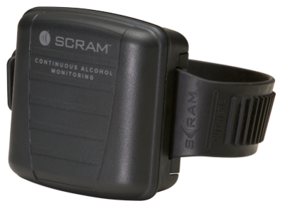
Currently, there are a number of different biosensors based on a variety of analog principles that can measure TAC essentially continuously, passively, unobtrusively, and relatively accurately, and make it available for processing in real time. Some of these devices are already commercially available and more are on the way. Several of these biosensors, like the breathalyzer, rely on relatively standard fuel-cell technology (i.e. converting chemical energy into electricity through redox reactions) to effectively count the number of ethanol molecules that evaporate during perspiration from the epidermal layer of the skin in near-continuous time Marques:2009. Figure (1) shows two of these TAC measuring devices; the WrisTAS^TM7, developed by Giner, Inc. in Waltham, MA and the SCRAM CAM^® (Secure Continuous Remote Alcohol Monitor), developed by Alcohol Monitoring Systems, Inc. (AMS) in Littleton, Colorado.

Historically, researchers, clinicians, and the courts have always relied on BrAC or, when available, BAC. Consequently, in order to make TAC biosensors practical and accepted by the alcohol community, reliable and consistent means for converting TAC into equivalent BrAC or BAC must be developed. However, unfortunately, as indicated previously, a number of challenges must be dealt with before this can be done. In the past, our approach to developing a method for converting TAC into BrAC or BAC was based on deterministic methods for estimating parameters in distributed parameter systems such as those described in Banks:1997; Banks:1989. Our earlier work along these lines has been reported in, for example, Dai:2016; Dumett:2008; Rosen:2014. In these treatments, a forward model in the form of a one-dimensional diffusion equation based on Fick’s law Smith:2004 with BrAC as the input and TAC as the output is first calibrated (i.e. fit) using BrAC and TAC data collected from the patient or research subject in the clinic or laboratory during what is known as a controlled alcohol challenge. Then, after the same patient or research subject has worn the TAC sensor in the field for an extended period of time (e.g. days, weeks, or even months), the TAC data is downloaded, and the fit forward model is used to deconvolve the BrAC or BAC input from the observed TAC output.

In order to eliminate the calibration process, we developed a population model-based approach wherein the parameters in the model were assumed to be random. Then, rather than fitting the values of the parameters themselves, their distributions were estimated based on BrAC and TAC data from a cohort of individuals (see, for example, Asserian:2021; Sirlanci:2019A; Sirlanci:2017; Sirlanci:2019B).

In all of our approaches to the TAC to BAC/BrAC conversion problem, the underlying model was taken to be based on the first principles physics based initial-boundary value problem for a parabolic partial differential equation. This will also be the basic model to which we will direct our efforts in the present treatment. Transformed to be in terms of dimensionless variables, the model is given by

where $t$ and $\eta$ are the temporal and spatial variables, respectively, and $x(t,\eta)$ indicates the concentration of ethanol in the epidermal layer of the skin at time $t$ and depth $\eta$, where $\eta=0$ is at the skin surface and $\eta=1$ is at the boundary between the epidermal and dermal layers of the skin. The input to the system is $u(t)$, which is the BrAC/BAC at time $t$, and the output is $y(t)$, which is the TAC at time $t$. Equation (1) represents the transport of ethanol through the epidermal layer of the skin. The boundary conditions (2) and (3) represent respectively the evaporation of ethanol at the skin surface and the flux of ethanol across the boundary between the epidermal and dermal layers. It is assumed that there is no alcohol in the epidermal layer of the skin at time $t=0$, so the initial condition (4) is $x_{0}(\eta)=0$, $0<\eta<1$. Finally, the output equation (5) represents the TAC level measured by the biosensor at the skin surface.

The parameters in the system (1)-(5) that will be assumed to be random are $q_{1}$ and $q_{2}$, which represent respectively the normalized diffusivity and the normalized flux gain at the boundary between the dermal and epidermal layers. The values or distributions of these parameters are assumed to depend on environmental conditions, the particular sensor being used, and the physiological characteristics of the individual wearing the sensor. The parameter vector is $\bm{q}=(q_{1},q_{2})\in Q$, where $Q$ is assumed to be a compact subset of $\mathbb{R}^{+}\times\mathbb{R}^{+}$ with metric $d$.

In population modeling, we can statistically classify the methods as parametric or nonparametric. In the parametric approach, we assume that the general structure of the distribution is known a-priori but with unknown parameters. Then, for example, if we know that the distribution is normal with unknown mean and variance, the estimation problem is to estimate these two unknown parameters. On the other hand; in the nonparametric approach, the structure of the distribution is assumed to be unknown, and the problem is to estimate the distribution itself. In either of these paradigms, different statistical approaches to the estimation problem can be taken. For example, in Sirlanci:2019A; Sirlanci:2017; Sirlanci:2019B, a parametric least squares naive pooled data approach was used, while in Asserian:2021; Banks:2012; Banks:2018A, the approach was nonparametric. In Hawekotte:2021, a Bayesian framework was developed, and in the present treatment we consider a mixed effects (see, for example, Davidian:1995; Davidian:2003; Demidenko:2013) maximum likelihood based statistical model. In the mixed effects model, it is assumed that observations are specific to a single individual plus a random error. The mixed effects model is a combination of the fixed-effects model, which describes the characteristics for an average individual in the population, and the random-effects model, which describes the inter-individual variability Lovern:2009. An overview of these different statistical approaches in the context of pharmacokinetics can be found in Tatarinova:2013.

In addition to the work of our group on TAC to BAC/BrAC conversion cited above, other researchers have also been looking at this problem and have tried a number of different approaches. For example, in Dougherty:2012; Dougherty:2015, a more traditional approach based on standard linear regression techniques is developed and discussed. A number of ideas from the machine learning literature have also been considered. In Fairbairn:2021, a scheme based on random forests is used to recover BrAC from TAC, and in our group, in Oszkinat:2021, the authors develop a method using physics-informed neural networks, and in Oszkinat:2021A, BrAC or BAC is estimated from observations of TAC using a Hidden Markov Model (HMM) based approach.

An outline of the remainder of the paper is as follows. In Section 2, we provide a summary of the Prohorov metric on the set of probability measures as it was used by Banks and his co-authors in Banks:2012. In Section 3, we define our mathematical model in the form of a random discrete-time dynamical system and we define the maximum likelihood estimator for the distribution of the random parameters. In the Section 4, we establish the existence and consistency of the maximum likelihood estimator, while in Section 5, we demonstrate the convergence of finite dimensional approximations for our estimator. In Section 6, we summarize results for abstract parabolic systems, their finite dimensional approximation, and an associated convergence theory. In Section 7, the application of our scheme to the transdermal transport of alcohol is presented and discussed. This includes numerical studies for two examples, one involving simulated data and the other, actual data collected in the laboratory of one of the co-authors, Dr. Susan Luczak, in the Department of Psychology at University of Southern California (USC). For the simulated data example in Section 7.1, we are able to observe the convergence of the estimated distribution of the random parameter vector $\bm{q}=(q_{1},q_{2})$ to the “true” distribution as the number of drinking episodes increases, as the number of Dirac measure nodes increases, and as the level of discretization in the finite dimensional approximations increases. We look at each case separately and in turn. In the actual data example discussed in Section 7.2, we apply the leave-one-out cross-validation (LOOCV) method by first estimating the distribution of the parameter vector $\bm{q}$ using a training set, and then estimating the TAC output using the estimated distribution and the BrAC input of a testing episode.

Banks and his co-authors developed a framework for estimation of the probability measure for random parameters in continuous-time dynamical systems based on the Prohorov metric Banks:2012. Here, we summarize the Prohorov metric and its properties.

Let $Q$ be a Hausdorff metric space with metric $d$. Define

and given any probability measure $P\in\mathcal{P}(Q)$, where $\mathcal{P}(Q)$ denotes the set of all probability measures defined on $\Sigma_{Q}$, the Borel sigma algebra on $Q$, and some $\epsilon>0$, an $\epsilon$-neighborhood of $P$ is defined by

Let $E\in\Sigma_{Q}$, and define the $\epsilon$-neighborhood of $E$ by

Given two probability measures, $P$ and $\tilde{P}$ in $\mathcal{P}(Q)$, the Prohorov metric $\rho$ on $\mathcal{P}(Q)\times\mathcal{P}(Q)$ is defined such that

where

It can be shown that $(\mathcal{P}(Q),\rho)$ is a metric space. Also, the Prohorov metric metrizes the weak convergence of measures, i.e. given a sequence of measures $P_{M}\in\mathcal{P}(Q)$, for all $M=1,2,\dots$, and $P\in\mathcal{P}(Q)$,

It is important to note that the weak^∗ topology and the weak topology are equivalent on the space of probability measures.

For some $n_{\bm{q}}$, $Q\subseteq\mathbb{R}^{n_{\bm{q}}}$ and $P\in\mathcal{P}(Q)$, consider the random vector $X:Q\rightarrow\mathbb{R}^{n_{\bm{q}}}$ on the probability space $(Q,\Sigma_{Q},P)$ given by $X(\bm{q})=\bm{q}$ for $\bm{q}\in Q$. The cumulative distribution function for $X$ is given by $F_{X}(q_{1},\dots,q_{n})=P(X\in\times_{\ell=1}^{n_{\bm{q}}}(-\infty,q_{\ell}])=P(\times_{\ell=1}^{n_{\bm{q}}}\{(-\infty,q_{\ell}]\cap Q\})$. In this case, it follows that if $\{P_{M}\},P_{0}\in(\mathcal{P}(Q)$, $\rho)$, then $\rho(P_{M},P_{0})\to 0$ if and only if $F_{X_{M}}\to F_{X_{0}}$ at all points of continuity of $F_{X_{0}}$. Consequently, Prohorov metric convergence and weak and weak^∗ convergence in $\mathcal{P}(Q)$ are also referred to as convergence in distribution.

If $\bm{q}_{1},\bm{q}_{2}\in Q$, then $\rho(\delta_{\bm{q}_{1}},\delta_{\bm{q}_{2}})=\min\{d(\bm{q}_{1},\bm{q}_{2}),1\}$, where $\delta_{\bm{q}_{j}}\in D=\{\delta_{\bm{q}}\enskip|\enskip\bm{q}\in Q\},$ the space of Dirac measures on $Q$, where for all $E\in\Sigma_{Q}$,

The metric space $(\mathcal{P}(Q),\rho)$ is separable if and only if the metric space $(Q,d)$ is separable. The sequence $\{\bm{q}_{j}\}_{j=1}^{\infty}$ is Cauchy in $(Q,d)$ if and only if the sequence $\{\delta_{\bm{q}_{j}}\}_{j=1}^{\infty}$ is Cauchy in $(\mathcal{P}(Q),\rho)$. We also have $(Q,d)$ is complete if and only if $(\mathcal{P}(Q),\rho)$ is complete, and $(Q,d)$ is compact if and only if $(\mathcal{P}(Q),\rho)$ is compact. The details and proofs can be found in Banks:2012.

Assume the metric space $(Q,d)$ is separable and let $Q_{d}=\{\bm{q}_{j}\}_{j=1}^{\infty}$ be a countable dense subset of $Q$. Define the dense (see Banks:2012) subset of $\mathcal{P}(Q)$, $\tilde{\mathcal{P}}_{d}(Q)$, as

the collection of all convex combinations of Dirac measures on $Q$ with rational weights $p_{j}$ at nodes $\bm{q}_{j}\in Q_{d}$, and for each $M\in\mathbb{N}$ let

Consider the following discrete-time mathematical model for the $i^{th}$ subject at time-step $k$

where $\bm{q}_{i}$ is the $i^{th}$ subject’s parameter vector in $Q$, denoting the set of admissible parameters, $g_{k-1}:\mathcal{H}\times\mathbb{R}^{\nu}\times Q\to\mathcal{H}$, $\mathcal{H}$ is in general an infinite dimensional Hilbert space, and $u_{k-1,i}\in\mathbb{R}^{\nu}$ is the input. The output is given by

where $h_{k}:\mathcal{H}\times\mathcal{H}\times\mathbb{R}^{\nu}\times Q\to\mathbb{R}$.

For the mixed effects model, we define

where for each $i=1,2,\dots,m$, $e_{k,i}$ are independent and identically distributed (i.i.d.) with mean $0$, variance $\sigma^{2}$, and $e_{k,i}\sim\varphi$, $k=1,2,\dots,n_{i}$, where $\varphi$ is a density with respect to a sigma finite measure $\mu$ on $\mathbb{R}$ and assumed to be continuous on $\mathbb{R}$, and we assume that the random vectors $[e_{1,i},\dots,e_{n_{i},i}]$ are independent with respect to $i$, $i=1,2,\dots,m$. That is, we assume that the error is independent across individuals and conditionally independent within individuals (i.e. given $\bm{q}_{i}$). For each $i=1,2,\dots,m$, let $\bm{Y}_{i}=[Y_{1,i},Y_{2,i},\dots,Y_{n_{i},i}]^{T}$, $\bm{y}_{i}(\bm{q}_{i})=[y_{1,i}(\bm{q}_{i}),y_{2,i}(\bm{q}_{i}),\dots,y_{n_{i},i}(\bm{q}_{i})]^{T}$, $\bm{e}_{i}=[e_{1,i},e_{2,i},\dots,e_{n_{i},i}]^{T}$ and rewrite (7) as

Then, for $i=1,2,\dots,m$, $\bm{Y}_{i}$ are independent with $\bm{Y}_{i}\sim f_{i}(\cdot;\bm{q}_{i}):\mathbb{R}^{n_{i}}\rightarrow\mathbb{R}$, where

where $\bm{v}=[v_{1},v_{2},\dots,v_{n_{i}}]^{T}\in\mathbb{R}^{n_{i}}$. Let $P\in\mathcal{P}(Q)$ denote a probability measure on the Borel sigma algebra on $Q$, $\Sigma_{Q}$, where $\mathcal{P}(Q)$ denotes the set of all probability measures defined on $\Sigma_{Q}$, and let $P_{0}\in\mathcal{P}(Q)$ be the “true” distribution of the random vector $\bm{q}_{i}$. The goal is to find an estimate of $P_{0}$. In order to generate an estimator for $P_{0}$, and establish theoretical results and computational tools, we use the nonparametric maximum likelihood (NPML) approach, introduced by Lindsay and Mallet in Lindsay:1983; Mallet:1986, using the Prohorov metric-based framework on $\mathcal{P}(Q)$, introduced by Banks and his co-authors in Banks:2012, and summarized in Section 2.

For $P\in\mathcal{P}(Q)$ and $i=1,2,\dots,m$, let

be the contribution of the $i^{th}$ subject to the likelihood function

where $\bm{n}=\{n_{i}\}_{i=1}^{m}$ and $\bm{Y}=\{\bm{Y}_{i}\}_{i=1}^{m}$. The goal is to find $P$ that maximizes the likelihood function. Define the estimator

Let ${\hat{y}}_{k,i}$ be realizations of the random variables $Y_{k,i}$, and define

where $\boldsymbol{{\hat{y}}}=\{{\boldsymbol{{\hat{y}}}}_{i}\}_{i=1}^{m}$, with ${\boldsymbol{{\hat{y}}}}_{i}=[{\hat{y}}_{1,i},{\hat{y}}_{2,i},\dots,{\hat{y}}_{n_{i},i}]^{T}$.

The results of Lindsay and Mallet in Lindsay:1983; Mallet:1986 states that the maximum likelihood estimator $\hat{P}_{\bm{n},m}$ can be found in the class of discrete distributions with at most $m$ support points, i.e. $\hat{P}_{\bm{n},m}\in\mathcal{P}_{M}(Q)$, where $M\leq m$.

We cannot exactly compute the maximum likelihood estimator, $\hat{P}_{\bm{n},m}$, since $y_{k,i}$ must be approximated numerically by $y^{N}_{k,i}$ using a Galerkin numerical scheme with $N$ denoting the level of discretization. Also, similarly, we define our approximating estimator over the set $\mathcal{P}_{M}(Q)$ where $M$ denotes the number of nodes, $\{\bm{q}_{j}\}_{j=1}^{M}$. As a result, the optimization is over a finite set of parameters, being the rational weights $\{p_{j}\}_{j=1}^{M}$. Thus, our approximating estimator is

In Lindsay:1983, the existence and uniqueness of a maximum likelihood estimator of a mixing distribution using the geometry of mixture likelihoods was established. Similarly, in Mallet:1986, the existence and uniqueness of the maximum likelihood estimator for the distribution of the parameters of a random coefficient regression model was established. Here we provide an existence argument based on the maximization of a continuous function over a compact set.

The following theorem establishes the existence of the estimator $\hat{P}_{\bm{n},m}$ in (13), obtained from the realizations $\{{\hat{y}}_{k,i}\},\enskip k=1,\dots,n_{i},\enskip i=1,\dots,m$ of the random variables $\{Y_{k,i}\},\enskip k=1,\dots,n_{i},\enskip i=1,\dots,m$. This is sufficient for establishing the existence of the maximum likelihood estimator $P_{\bm{n},m}$ in (11).

In order to establish the consistency of the maximum likelihood estimator $P_{\bm{n},m}$, we show that $\rho(P_{\bm{n},m},P_{0})$ converges almost surely to zero. We do this by applying a theorem by Kiefer and Wolfowitz in Kiefer:1956, establishing that the nonparametric maximum likelihood approach is statistically consistent. In other words, as the number of subjects, $m$, gets larger, the estimator $P_{\bm{n},m}$ converges in probability to $P_{0}$, the “true” distribution, in the sense of the Prohorov metric, or weakly, or in distribution. Here, we have set up our problem in a way that makes establishing the consistency a straightforward application of the consistency result in Kiefer:1956.

We want to establish the convergence of the finite dimensional maximum likelihood estimators to the maximum likelihood estimator corresponding to the infinite dimensional model. As mentioned earlier, we cannot actually compute $\hat{P}_{\bm{n},m}$ in (12) and consequently we approximate it by $\hat{P}_{\bm{n},m,M}^{N}$ in (13). Consider the following assumptions,

• A1.

  For all $\bm{n}$, $m$, and $N$, the map $P\mapsto\mathcal{L}_{\bm{n},m}^{N}(P;\boldsymbol{{\hat{y}}})$ is a continuous map.

• A2.

  For any $\{P_{M}\},P\in\mathcal{P}(Q)$ such that $\rho(P_{M},P)\to 0$, we have $\mathcal{L}_{i}^{N}(P_{M};\boldsymbol{{\hat{y}}}_{i})\to\mathcal{L}_{i}(P;\boldsymbol{{\hat{y}}}_{i})$ as $N,M\to\infty$ for $i=1,\dots,m$.

• A3.

  For all $P\in\mathcal{P}(Q)$ and $i=1,\dots,m$, $\mathcal{L}_{i}^{N}(P_{M};\boldsymbol{{\hat{y}}}_{i})$ and $\mathcal{L}_{i}(P;\boldsymbol{{\hat{y}}}_{i})$ are uniformly bounded.

In practice, to achieve a desired level of accuracy, $M$ and $N$ are fixed sufficiently large. We choose a sufficiently large value for $N$, how large that needs to be, of course, depends on the particular numerical discretization scheme chosen. The most common choice would be using a Galerkin-based method to the approximate ${y}_{k,i}$ by ${y}_{k,i}^{N}$. We also choose a sufficiently large value for $M$, the number of nodes, $\{\bm{q}_{j}\}_{j=1}^{M}$. Therefore, the optimization problem is reduced to a standard constrained estimation problem over Euclidean $M$-space, in which we determine the values of the weights $p_{j}$ at each node $\bm{q}_{j}$ with the constraints that they all be non-negative and sum to one. By equation (13). It follows that

where $\tilde{\bm{p}}=(p_{1},\dots,p_{M})\in\widetilde{\mathbb{R}^{M}}=\{\tilde{\bm{p}}\enskip|\enskip p_{j}\in\mathbb{R}^{+},\sum_{j=1}^{M}p_{j}=1\}$.

We note that computing $\hat{P}_{\bm{n},m,M}^{N}$ involves high order products of very small numbers which not unexpectedly can cause numerical underflow. In order to mitigate this, we maximize the log-likelihood function instead and rewrite it in a form that lends itself to the use of the MATLAB optimization routine logsumexp as follows

In order to apply our estimation theory to equations (1)-(5), our model for the transdermal transport of ethanol given in Section 1, we reformulate it as an abstract parabolic system. We briefly describe what an abstract parabolic system is, its properties, and its finite dimensional approximation, and then we show how assumptions A1-A3 are satisfied for such a system.

Let $H$ and $V$ be Hilbert spaces with $V$ densely and continuously embedded in $H$. Pivoting on $H$, it follows that $H$ is therefore densely and continuously embedded in the dual of $V$, $V^{*}$. This is known as a Gelfand triple and is generally written as $V\hookrightarrow H\hookrightarrow V^{*}$ Tanabe:1979. Then an abstract parabolic system is a dynamical system of the following form

where $<\cdot,\cdot>_{V^{*},V}$ denotes the duality pairing between $V^{*}$ and $V$, $Q$ is as defined in Section 1, and for each $\bm{q}\in Q$, $a(\bm{q};.,.):V\times V\to\mathbb{C}$ is a sesquilinear form satisfying the following three assumptions,

• B1.

  (Boundedness) There exists a constant $\alpha_{0}$ such that for all $\psi_{1},\psi_{2}\in V$, we have

  $\displaystyle|a(\bm{q};\psi_{1},\psi_{2})|\leq\alpha_{0}\parallel\psi_{1}\parallel_{V}\parallel\psi_{2}\parallel_{V}.$

• B2.

  (Coercivity) There exists $\lambda_{0}\in\mathbb{R}$ and $\mu_{0}>0$ such that for all $\psi\in V$, we have

  $\displaystyle a(\bm{q};\psi,\psi)+\lambda_{0}|\psi|_{H}^{2}\geq\mu_{0}\parallel\psi\parallel_{V}^{2}.$

• B3.

  (Continuity) For all $\psi_{1},\psi_{2}\in V$ and $\bm{q},\tilde{\bm{q}}\in Q$, we have

  $$|a(\bm{q},\psi_{1},\psi_{2})-a(\tilde{\bm{q}},\psi_{1},\psi_{2})|\leq d(\bm{q},\tilde{\bm{q}})\parallel\psi_{1}\parallel_{V}\parallel\psi_{2}\parallel_{V}.$$

In these assumptions, $\parallel.\parallel_{V}$ and $|.|_{H}$ denotes the norm on the spaces $V$ and $H$, respectively. Further, in (16), $\bm{B}(\bm{q}):\mathbb{R}^{\nu}\to V^{*}$, and $\bm{C}(\bm{q}):V\to\mathbb{R}$ are bounded linear operators with initial conditions $x_{0}\in H$, input $u\in L^{2}([0,T],\mathbb{R}^{\nu})$, and output $y\in L^{2}([0,T],\mathbb{R})$.

References

- (1) Adams, R.A., Fournier, J.J.F.: Sobolev Spaces. (2003)
- (2) Asserian, L., Rosen, I.G., Luczak, S.E.: Prohorov metric-based nonparametric estimation of random parameters in abstract parabolic systems with application to the transdermal transport of alcohol. submitted. (2021)
- (3) Banks, H.T., Flores, K.B., Rosen, I.G., Rutter, E.M., Sirlanci, M., Thompson, W.C.: The prohorov metric framework and aggregate data inverse problems for random PDEs. Communications in Applied Analysis. 22(3), 415-446 (2018)
- (4) Banks, H.T., Ito, K.: A unified framework for approximation in inverse problems for distributed parameter systems. NASA. Hampton, VA. Technical Reports NASA-CR-181621 (1988)
- (5) Banks, H.T., Ito, K.: Approximation in LQR problems for infinite dimensional systems with unbounded input operators. Journal of Mathematical Systems, Estimation and Control. 7, 1-34 (1997)
- (6) Banks, H.T., Kunisch, K.: Estimation Techniques for Distributed Parameter Systems. Birkhauser, Boston (1989)
- (7) Banks, H.T., Kunisch, K.: The linear regulator problem for parabolic systems. SIAM Journal on Control and Optimization. 22(5), 684-698 (1984)
- (8) Banks, H.T., Thompson, W.C.: Least Squares Estimation of Probability Measures in the Prohorov Metric Framework. Technical report, DTIC (2012)
- (9) Banks, H.T., Flores, K.B., Rosen, I.G., Rutter, E.M., Sirlanci, M. and Thompson, W. C.: The Prohorov metric framework and aggregate data inverse problems for random PDEs, Communications in Applied Analysis, 22(3), 415-446 (2018)
- (10) Dai, Z., Rosen, I.G., Wang, C., Barnett, N.P., Luczak, S.E.: Using drinking data and pharmacokinetic modeling to calibrate transport model and blind deconvolution-based data analysis software for transdermal alcohol biosensors. Mathematical Biosciences and Engineering. 13, 911-934 (2016)
- (11) Davidian, M., Giltinan, D.: Nonlinear Models for Repeated Measurement Data. Chapman and Hall, New York (1995)
- (12) Davidian, M., Giltinan, D. M.: Nonlinear models for repeated measurement data: An overview and update. Journal of Agricultural, Biological, and Environmental Statistics. 8, 387-419 (2003)
- (13) Demidenko, E.: Mixed models, theory and applications (2nd ed.). John Wiley and Sons, Hoboken (2013)
- (14) Dougherty, D.M., Charles, N.E., Acheson, A., John, S., Furr, R.M., and Hill-Kapturczak, N.: Comparing the detection of transdermal and breath alcohol concentrations during periods of alcohol consumption ranging from moderate drinking to binge drinking, Exp. Clin. Psychopharm. 20, 373-81 (2012)
- (15) Dougherty, D.M., Karns, T.E., Mullen, J., Liang, Y., Lake, S.L., Roache, J.D., and Hill-Kapturczak, N.: Transdermal alcohol concentration data collected during a contingency management program to reduce at-risk drinking, Drug and Alc. Dep. 148, 77-84 (2015)
- (16) Dumett, M.A., Rosen, I.G., Sabat, J., Shaman, A., Tempelman, L., Wang, C., and Swift, R.: Deconvolving an estimate of breath measured blood alcohol concentration from biosensor collected transdermal ethanol data, Applied Mathematics and Computation. 196(2), 724-743 (2008)
- (17) Fairbairn, C.E., Kang, D., and Bosch, N.: Using machine learning for real-time BAC estimation from a new-generation transdermal biosensor in the laboratory, Drug and Alc. Dep. 216, 108205 (2021)
- (18) Hawekotte, K., Luczak, S. E., and Rosen, I. G.: A Bayesian approach to quantifying uncertainty in transport model parameters for, and breath alcohol concentration deconvolved from, biosensor measured transdermal alcohol level, submitted. (2021)
- (19) Kiefer, J., Wolfowitz, J.: Consistency of the maximum likelihood estimator in the presence of infinitely many incidental parameters. Annals of Mathematical Statistics. 27(4), 887-906 (1956)
- (20) Labianca, D.A.: The chemical basis of the breathalyzer. Journal of Chemical Education. 67(3), 259-261 (1990)
- (21) Lindsay, B.: The geometry of mixture likelihoods: a general theory. Ann Stat. 11, 86-94 (1983)
- (22) Lions, J.L.: Optimal Control of Systems Governed by Partial Differential Equations. Grundlehren der mathematischen Wissenschaften in Einzeldarstellungen mit besonderer Berucksichtigung der Anwendungsgebiete. Springer-Verlag (1971)
- (23) Lovern, M., Sargentini-Maier, M., Otoul, C., Watelet, J.: Population pharmacokinetic and pharmacodynamic analysis in allergic diseases. Drug Metabolism Reviews. 41(3), 475-485 (2009)
- (24) Luczak, S.E., Rosen, I.G., Wall, T.L.: Development of a real-time repeated-measures assessment protocol to capture change over the course of drinking episodes. Alcohol and Alcoholism. 50, 1-8 (2015)
- (25) Mallet, A.: A maximum likelihood estimation method for random coefficient regression models. Biometrika. 73(3), 645-656 (1986)
- (26) Marques, P.R., McKnight, A.S.: Field and laboratory alcohol detection with 2 types of transdermal devices. Alcoholism: Clinical and Experimental Research. 33(4), 703-711 (2009)
- (27) Oszkinat, C., Luczak, S.E. and Rosen, I.G.: Uncertainty quantification in the estimation of blood alcohol concentration using physics-informed neural networks. submitted. (2021)
- (28) Oszkinat, C., Shao, T., Wang, C., Rosen, I.G., Rosen, A.D., Saldich, E. and Luczak, S.E.: A covariate-dependent hidden Markov model for uncertainty quantification and estimation of blood and breath alcohol concentration from transdermal alcohol biosensor data. submitted. (2021)
- (29) Pazy, A.: Semigroups of Linear Operators and Applications to Partial Differential Equations. New York Springer (1983)
- (30) Rosen, I.G., Luczak, S.E., Weiss, J.: Blind deconvolution for distributed parameter systems with unbounded input and output and determining blood alcohol concentration from transdermal biosensor data. Applied Math and Computation. 231, 357-376 (2014)
- (31) Sakai, J.T., Mikulich-Gilbertson, S.K., Long, R.J., Crowley, T.J.: Validity of transdermal alcohol monitoring: fixed and self-regulated dosing. Alcoholism: Clinical and Experimental Research. 30(1), 26-33 (2006)
- (32) Saldich, E.B., Wang, C., Rose, I.G., Goldstein, L., Bartroff, J., Swift, R.M., Luczak, S.E.: Obtaining high-resolution multi-biosensor data for modeling transdermal alcohol concentration data. Alcoholism: Clinical and Experimental Research. 44(1), 181A (2020)
- (33) Schultz, M.H.: Spline Analysis. Prentice-Hall (1973)
- (34) Sirlanci, M., Luczak, S.E., Fairbairn, C.E., Kang, D., Pan, R., Yu, X., Rosen, I.G.: Estimating the distribution of random parameters in a diffusion equation forward model for a transdermal alcohol biosensor. Automatica. 106, 101-109 (2019)
- (35) Sirlanci, M., Luczak, S.E., Rosen, I.G.: Approximation and convergence in the estimation of random parameters in linear holomorphic semigroups generated by regularly dissipative operators. American Control Conference (ACC). 3171-3176 (2017)
- (36) Sirlanci, M., Luczak, S.E., Rosen, I.G.: Estimation of the distribution of random parameters in discrete time abstract parabolic systems with unbounded input and output: approximation and convergence. Communications in Applied Analysis. 23(2), 287-329 (2019)
- (37) Sirlanci, M., Rosen, I.G., Luczak, S.E., Fairbairn, C.E., Bresin, K., Kang, D.: Deconvolving the input to random abstract parabolic systems: a population model-based approach to estimating blood/breath alcohol concentration from transdermal alcohol biosensor data. Inverse Problems. 34, 125006 (27pp) (2018)
- (38) Smith, W.F., Hashemi, J., Presuel-Moreno, F.: Foundations of Materials Science and Engineering. McGraw-Hill, New York, NY, 3rd edition (2004)
- (39) Swift, R.M.: Transdermal alcohol measurement for estimation of blood alcohol concentration. Alcoholism: Clinical and Experimental Research. 24(4), 422-423 (2000)
- (40) Tanabe, H.: Equations of Evolution. Monographs and Studies in Mathematics. Pitman (1979)
- (41) Tatarinova, T., Neely, M., Bartroff, J., van Guilder, M., Yamada, W., Bayard, D., Jelliffe, R., Leary, R., Chubatiuk, A., Schumitzky, A.: Two general methods for population pharmacokinetic modeling: non-parametric adaptive grid and non-parametric Bayesian. J Pharmacokinet Pharmacodyn. 40, 189-199 (2013)