跳到论文正文
W Papers独立论文阅读器 arXiv:2304.12011 论文正文 计算阅读时间 · 0%
引用这篇论文根据当前论文元数据生成,正式投稿前建议核对。


License: CC BY 4.0
arXiv:2304.12011v1 [hep-th] 24 Apr 2023

.

On the ultraviolet behavior of conformally reduced quadratic gravity

Alfio Bonanno Email: alfio.bonanno@inaf.it Affiliation: INAF, Osservatorio Astrofisico di Catania, via S.Sofia 78, I-95123 Catania, Italy    Maria Conti Email: mconti@uninsubria.it Affiliation: DISAT, Università degli Studi dell’Insubria, via Valleggio 11, I-22100 Como, Italy
INFN, Sezione di Milano, Via Celoria 16, I-20133 Milano, Italy
   Sergio Cacciatori Email: sergio.cacciatori@uninsubria.it Affiliation: DISAT, Università degli Studi dell’Insubria, via Valleggio 11, I-22100 Como, Italy
INFN, Sezione di Milano, Via Celoria 16, I-20133 Milano, Italy
Abstract

We study the conformally reduced R+R2R+R^{2} theory of gravity and we show that the theory is asymptotically safe with an ultraviolet critical manifold of dimension three. In particular, we discuss the universality properties of the fixed point and its stability under the use of different regulators with the help of the proper-time flow equation. We find three relevant directions, corresponding to the g\sqrt{g}, g​R\sqrt{g}R and g​R2\sqrt{g}R^{2} operators, whose critical properties are very similar to the ones shared by the full theory. Our result shows that the basic mechanism at the core of the Asymptotic Safety program is still well described by the conformal sector also beyond the Einstein-Hilbert truncation. Possible consequences for the asymptotic safety program are discussed.

I Introduction

Despite the fact that the Asymptotically Safe approach to quantum gravity is a relatively new approach to the quantization of the gravitational field, the basic assumptions of this approach are deeply rooted in old-fashioned, standard Quantum Field Theory. The basic idea at the core of this program is that, as long as we do not insist on the notion of continuum limit tailored to perturbation theory, gravity can be treated along the same lines as similar quantum field theories whose continuum limit is defined non-perturbatively. This possibility was first suggested by Weinberg Weinberg 1979 and further implemented by Reuter Reuter 1998 by means of the Wilsonian renormalization group (RG) formalism in Quantum Field Theory (QFT) Niedermaier and Reuter 2006; Bonanno 2011; Litim 2011; Nagy 2014; Eichhorn 2018; Pereira 2019; Reichert 2020; Bonanno et al. 2020; Platania 2020. (See the recent books Percacci 2017; Reuter and Saueressig 2019 for a pedagogical introduction to the subject.)

It is possible to explain the technical mechanism which lies at the root of the non-perturbative renormalization of Einstein’s gravity in simple physical terms. Perhaps the most illuminating discussion in this context has been presented by Polyakov Polyakov 1993, who noticed that as gravity is always attractive and therefore a larger cloud of virtual particle implies a stronger gravitational force, Newton’s constant GG should be antiscreened at small distances. The implication of this behaviour suggests that the dimensionless coupling constant g⁡(ℓ)=G⁡(ℓ)/ℓ2g(\ell)=G(\ell)/\ell^{2} tends to a finite non-zero limit at small distances

limℓ→0g⁡(ℓ)∝g∗≠0\lim_{\ell\rightarrow 0}g(\ell)\propto g^{\ast}\not=0 (1)

as GG scales as ℓ2\ell^{2} according to its natural dimensions. A theory whose dimensionless coupling constant approaches a non-Gaussian (non-vanishing) fixed point (NGFP) in the short distance limit as in (1) is called asymptotically safe (at variance with the more familiar case of the asymptotic freedom where g∗=0g^{\ast}=0.)

In a series of papers Reuters and collaborators have clarified that conformal factor plays a central role in the emergence of the NGFP in the ultraviolet region and in the determination of the critical properties of the theory Reuter and Weyer 2009a; Reuter and Weyer 2009b; Manrique et al. 2011. There are two issues in particular which make the emergence of 1 highly non-trivial, the first one is the use of the background field approach, and the second is the pivotal role played by the conformal field instability. In fact, the central idea of conformal field quantization is to employ the background metric (in the sense of the background field method) in constructing the Wilsonian renormalization group equations. On the other hand, as the conformal factor has the wrong kinetic sign in the euclidean theory, a special regulator must be employed to cutoff modes with the “wrong” ultraviolet stability properties. As first discussed in Bonanno and Guarnieri 2012, the IR evolution of the renormalization trajectory can be problematic and only an ultraviolet evolution can be consistently defined. Most probably a new kind of perturbative continuum limit for quantum gravity emerges in the deep UV for the conformally reduced theory, in this case, Mitchell and Morris 2020.

The role of the conformal degrees of freedom in determining the presence of the NGFP has been discussed for pure R2R^{2} in Machado and Percacci 2009. The authors found that the fixed point disappears for pure gravity but is present when matter is included. In four dimensions the question was further discussion in a conformally reduced version of the f⁡(R)f(R) theory in Demmel et al. 2015 . The authors found a scaling solution with properties qualitatively very similar to the ones constructed from the full flow equation obtained using a smooth approximation to the full spectrum of the hyperspherical harmonics. More recently the existence of the NGFP for the conformally reduced R+R2R+R^{2} theory has been questioned in Knorr 2021 a flat-space derivative expansion combined with an exponential parametrisation for the fluctuations of the conformal factor has been used.

In this work, close in spirit to the original Lauscher and Reuter 2002 calculation, we consider a conformally reduced R+R2R+R^{2} theory with a linear parametrization for conformal factor fluctuations, and a compact background projection. We find that the NGFP is clearly present and, more importantly, the universal properties of the UV critical manifold of the reduced theory are very similar to those shared by the full quadratic theory. Our conclusion is that the role of the other degrees of freedom of the metric is mostly relevant for the actual location of the fixed point in the space of the coupling constants, but it plays no significant role in deciding the universal properties of the theory.

II Functional flow equation for the conformal factor

It is instructive to clarify the main steps in the derivation of the flow equation for the conformal factor. In fact despite the fact that formally one deals with a scalar theory, the requirement of background independence plays an important role in the definition of the regulator.

Let S⁡[χ]S[\chi] be the action for the fundamental field χ⁡(x)\chi(x) that we write as χ⁡(x)=χB​(x)+f⁡(x)\chi(x)=\chi_{B}(x)+f(x) where χB​(x)\chi_{B}(x) is a non-dynamical background field and f⁡(x)f(x) a dynamical (fluctuating) field. In this formalism χ\chi plays the same role of a microscopic metric γμ​ν\gamma_{\mu\nu} in the full theory. In the complete framework a background metric g¯μ​ν\bar{g}_{\mu\nu} is chosen in order to perform the actual calculations, and the fluctuations hμ​νh_{\mu\nu} are thus “integrated-out” in momentum shell (in the wilsonian approach). The background should be dynamically determined by the requirement that the expectation value of the fluctuation field vanishes, ⟨hμ​ν⟩≡h¯μ​ν=0\langle h_{\mu\nu}\rangle\equiv\bar{h}_{\mu\nu}=0. Any physical length must then be proper with respect to the background metric g¯μ​ν\bar{g}_{\mu\nu}. In the conformally reduced theory the expectation values f¯≡⟨f⟩\bar{f}\equiv\langle f\rangle and ϕ≡⟨χ⟩=χB+f¯\phi\equiv\langle\chi\rangle=\chi_{B}+\bar{f} are the analogs of h¯μ​ν≡⟨hμ​ν⟩\bar{h}_{\mu\nu}\equiv\langle h_{\mu\nu}\rangle and gμ​ν=⟨γμ​ν⟩=g¯μ​ν+h¯μ​νg_{\mu\nu}=\langle\gamma_{\mu\nu}\rangle=\bar{g}_{\mu\nu}+\bar{h}_{\mu\nu} in the full theory.

The central idea of the conformal field quantization is to employ the background metric

g¯μ​ν=χB2​ν​g^μ​ν\bar{g}_{\mu\nu}=\chi_{B}^{2\nu}\,\hat{g}_{\mu\nu} (2)

where g^μ​ν\hat{g}_{\mu\nu} is a reference metric which plays no dynamical role but it is instead fixed to perform the actual calculations on the geometry defined by g¯\bar{g}. The momentum scale kk is therefore a “proper”-g¯μ​ν\bar{g}_{\mu\nu} momentum scale defined from the eigenvalues of the −□¯-\bar{\Box} operator. Therefore

k¯2=χB−2​ν​k2\bar{k}^{2}=\chi_{B}^{-2\,\nu}\,k^{2} (3)

in the case of a constant χB\chi_{B}. As discussed in Reuter and Weyer 2009a; Bonanno and Guarnieri 2012 the difference Δ​SkB=Skb+δ​kB−SkB\Delta S_{k_{B}}=S_{k_{b}+\delta k_{B}}-S_{k_{B}} can then be evaluated in the infinitesimal momentum shell between kBk_{B} and kB+δ​kBk_{B}+\delta k_{B}, where kBk_{B} is the “proper” momentum operator built with the background metric g¯μ​ν\bar{g}_{\mu\nu}. A functional flow equation is finally obtained by taking the δ​kB→0\delta k_{B}\rightarrow 0 limit and performing a renormalization group improvement of the resulting expression. After this step is accomplished, the “background-independent” flow is obtained expressing all the running “proper” momenta in terms of the reference energy scale kk. Rewriting the (regularized) one-loop contribution in the Schwinger “proper-time” formalism one finds

∂tSk[f;χB]=−12Tr∫0∞d​ss∂tρkexp{−sδ2​Sk​[f;χB]δ​f2},\partial_{t}\,{S}_{k}[f;\chi_{B}]=-\frac{1}{2}\,{\rm Tr}\int_{0}^{\infty}\frac{ds}{s}\,\partial_{t}\,\rho_{k}\,\exp\Big\{-s\frac{\delta^{2}S_{k}[f;\chi_{B}]}{\delta{f}^{2}}\Big\}\,, (4)

where t≡log⁡(k)t\equiv\log(k) is the RG time and ρk=ρk​[χB]\rho_{k}=\rho_{k}[\chi_{B}]. The important difference between this type of functional “proper-time” flow equation and the version used in earlier investigations is that the trace in (4) is here computed by means of the representation provided by the spectrum of −□¯-\bar{\Box},

Tr¯​[A]≡∫dd​x​g¯​⟨x|A|x⟩=∫dd​x​g^​χBd​ν​⟨x|A|x⟩.\overline{{\rm Tr}}[A]\equiv\int d^{d}x\,\sqrt{\bar{g}}\,\,\langle x|A|x\rangle=\int d^{d}x\,\sqrt{\hat{g}}\,\chi_{B}^{d\nu}\,\langle x|A|x\rangle\,. (5)

For actual calculations we shall use various families of smooth cutoffs ρk≡ρk1,2​(s,n)\rho_{k}\equiv\rho_{k}^{1,2}(s,n) that have been widely used in the literature Bonanno and Guarnieri 2012; Bonanno and Reuter 2005; Litim and Zappala 2011 whose explicit expressions are

ρk1​(s,n)=Γ⁡(n,s​𝒵​k^2)−Γ⁡(n,s​𝒵​Λ2)Γ⁡(n)\displaystyle\rho_{k}^{1}(s,n)=\frac{\Gamma(n,s\,{\cal Z}\,\hat{k}^{2})-\Gamma(n,s\,{\cal Z}\,\Lambda^{2})}{\Gamma(n)} (6)
ρk2​(s,n)=Γ⁡(n,s​n​𝒵​k^2)−Γ⁡(n,s​n​𝒵​Λ2)Γ⁡(n).\displaystyle\rho_{k}^{2}(s,n)=\frac{\Gamma(n,s\,n\,{\cal Z}\,\hat{k}^{2})-\Gamma(n,s\,n\,{\cal Z}\,\Lambda^{2})}{\Gamma(n)}. (7)

Here nn is an arbitrary real, positive parameter that controls the shape of the ρk1,2​(s,n)\rho_{k}^{1,2}(s,n) in the interpolating regions, and Γ⁡(α,x)=∫x∞d​t​tα−1​e−t\Gamma(\alpha,x)=\int^{\infty}_{x}dt\;t^{\alpha-1}e^{-t} denotes the incomplete Gamma-function. Furthermore, 𝒵{\cal Z} is a constant which has to be adjusted: being the kinetic terms of the field of type aa of the form −Za​□^-Z_{a}\hat{\Box}, we impose exactly 𝒵=Za{\cal Z}=Z_{a}. With this prescription, in (6) the eigenvalues of □^\hat{\Box} are cut off at ∼k^2\sim\hat{k}^{2}, instead of ∼k^2/Za\sim\hat{k}^{2}/Z_{a}. Similarly, in (7) the cutoff is located at ∼k^2/n\sim\hat{k}^{2}/n. These two choices represent two so-called ‘spectral adjustments’. Moreover, as background independence must be achieved, the trace inside the flow equation (4) must be performed on the modes of the background g¯μ​ν\bar{g}_{\mu\nu}. This is concretely performed inside the regularizators through the identification k^2=χB2​ν​k¯2\hat{k}^{2}=\chi_{B}^{2\nu}\bar{k}^{2}. Finally, Λ\Lambda represents the cutoff in the UV. As we are interested only in the Wilson-Kadanoff portion of the RG, the UV cut-off is sent to infinity. Overall, this leads to implementing the scaling laws

∂tρk1​(s,n)=−2Γ⁡(n)​(s​Z​k2​χB2​ν)n​e−s​Z​k2​χB2​ν.\displaystyle\partial_{t}\rho^{1}_{k}(s,n)=-\frac{2}{\Gamma(n)}(s\,Z\,k^{2}\,\chi_{B}^{2\nu})^{n}e^{-s\,Zk^{2}\chi_{B}^{2\nu}}. (8)
∂tρk2​(s,n)=−2Γ⁡(n)​(s​n​Z​k2​χB2​ν)n​e−s​n​Z​k2​χB2​ν\displaystyle\partial_{t}\rho^{2}_{k}(s,n)=-\frac{2}{\Gamma(n)}(s\,n\,Zk^{2}\,\chi_{B}^{2\nu})^{n}e^{-s\,nZk^{2}\chi_{B}^{2\nu}} (9)

inside the flow equation. Concretely, the calculations for both cutoff families are performed through a range of values for the smoothness parameter nn: n={3,5,7,9,10,15,20,30,40,50}{n=\left\{3,5,7,9,10,15,20,30,40,50\right\}}. The limiting case n→∞{n\to\infty} is also considered for the second regularizator: this is readily done through the already known identity Bonanno and Lacagnina 2004

limn→∞∂tρk(2)​(s,n)=−2Z​k2​χB2​ν​δ​(s−1Z​k2​χB2​ν).\lim_{n\to\infty}\partial_{t}\rho^{(2)}_{k}(s,n)=-\frac{2}{Z\,k^{2}\,\chi_{B}^{2\nu}}\delta\left(s-\frac{1}{Z\,k^{2}\,\chi_{B}^{2\nu}}\right). (10)

Finally, as an extra check for the robustness of the physical results under a change in the regularizator shapes, a slight modification in the cutoff structure ρk1,2\rho_{k}^{1,2} is also studied. Cutoffs (8) and (9) are built through the regularization on k¯2\bar{k}^{2}, which are the modes of the −□¯-\bar{\Box} operator. Because our model (described in detail in Section III) contains both −□¯-\bar{\Box} and □¯2\bar{\Box}^{2} operators, following the reasonings of Buccio and Percacci 2022, we also apply a regularization on the quadratic operator in order to check possible differences in the physics of the results. New cutoffs are defined:

ρ~k1​(s,n)=Γ⁡(n,s⁡(Z​k^2+Z2​k^4))−Γ⁡(n,s⁡(Z​Λ2+Z2​Λ4))Γ⁡(n)\displaystyle\tilde{\rho}_{k}^{1}(s,n)=\frac{\Gamma(n,s\,(Z\hat{k}^{2}+Z^{2}\hat{k}^{4}))-\Gamma(n,s\,(Z\Lambda^{2}+Z^{2}\Lambda^{4}))}{\Gamma(n)} (11)
ρ~k2​(s,n)=Γ⁡(n,s​n​(Z​k^2+Z2​k^4))−Γ⁡(n,s​n​(Z​Λ2+Z2​Λ4))Γ⁡(n),\displaystyle\tilde{\rho}_{k}^{2}(s,n)=\frac{\Gamma(n,s\,n\,(Z\hat{k}^{2}+Z^{2}\hat{k}^{4}))-\Gamma(n,s\,n\,(Z\Lambda^{2}+Z^{2}\Lambda^{4}))}{\Gamma(n)}, (12)

Requiring background independence by cutting the modes of the background metric and sending the UV cutoff Λ→∞\Lambda\to\infty leads to the the following scaling laws:

∂tρ~k1(s,n)=−2Γ⁡(n)(s(Zk2χB2​ν+Z2k4χB4​ν))n×\displaystyle\partial_{t}\tilde{\rho}^{1}_{k}(s,n)=-\frac{2}{\Gamma(n)}(s\,(Zk^{2}\chi_{B}^{2\nu}+Z^{2}k^{4}\chi_{B}^{4\nu}))^{n}\times
×e−s⁡(Z​k2​χB2​ν+Z2​k4​χB4​ν).\displaystyle\hskip 9.24994pt\hskip 9.24994pt\hskip 9.24994pt\hskip 9.24994pt\hskip 9.24994pt\hskip 9.24994pt\times e^{-s\,(Zk^{2}\chi_{B}^{2\nu}+Z^{2}k^{4}\chi_{B}^{4\nu})}. (13)
∂tρ~k2(s,n)=−2Γ⁡(n)(sn(Zk2χB2​ν+Z2k4χB4​ν))n×\displaystyle\partial_{t}\tilde{\rho}^{2}_{k}(s,n)=-\frac{2}{\Gamma(n)}(s\,n\,(Zk^{2}\chi_{B}^{2\nu}+Z^{2}k^{4}\chi_{B}^{4\nu}))^{n}\times
×e−s​n​(Z​k2​χB2​ν+Z2​k4​χB4​ν).\displaystyle\hskip 9.24994pt\hskip 9.24994pt\hskip 9.24994pt\hskip 9.24994pt\hskip 9.24994pt\hskip 9.24994pt\times e^{-s\,n\,(Zk^{2}\chi_{B}^{2\nu}+Z^{2}k^{4}\chi_{B}^{4\nu})}. (14)

III Non-perturbative β\beta-functions

In this section implement the RG flow equation approach to study the conformal sector of the the following theory:

S=∫dd​x​g​[116​π​G​(−R+2​Λ)+β​R2].S=\int d^{d}x\sqrt{g}\left[\frac{1}{16\pi G}(-R+2\Lambda)+\beta R^{2}\right]. (15)

A Weyl rescaling gμ​ν=ϕ​(x)2​ν​g^μ​νg_{\mu\nu}=\phi(x)^{2\nu}\hat{g}_{\mu\nu} is implemented, where ν=2/(d−2)\nu=2/(d-2) and g^μ​ν\hat{g}_{\mu\nu} is a reference metric. Weyl rescaling leads to

R=ϕ−2​ν​(R^−2​ν​(d−1)​□^​ϕϕ+g⁡(d)​g^μ​ν​∂μϕ​∂νϕϕ2),\displaystyle R=\phi^{-2\nu}\left(\hat{R}-\frac{2\nu(d-1)\hat{\Box}\phi}{\phi}+g(d)\frac{\hat{g}^{\mu\nu}\partial_{\mu}\phi\partial_{\nu}\phi}{\phi^{2}}\right), (16)

where g⁡(d)=(2​ν​(d−1)−ν2​(d−1)​(d−2))=0{g(d)=\left(2\nu(d-1)-\nu^{2}(d-1)(d-2)\right)=0} as ν=2/(d−2){\nu=2/(d-2)} and R^=R⁡(g^){\hat{R}=R(\hat{g})}. Being the scaling of the metric g=ϕd​ν​g^\sqrt{g}=\phi^{d\nu}\sqrt{\hat{g}}, the effective action is

Γk=∫dd​x​g^\displaystyle\Gamma_{k}=\int d^{d}x\sqrt{\hat{g}} [−12Zkϕ□^ϕ+U[ϕ]+\displaystyle\left[-\frac{1}{2}Z_{k}\phi\hat{\Box}\phi+U[\phi]+\right.
+16​(d−1d−2)2​βk​(□^​ϕ)2​ϕ2​d−8d−2−2+\displaystyle+16\left(\frac{d-1}{d-2}\right)^{2}\beta_{k}(\hat{\Box}\phi)^{2}\phi^{\frac{2d-8}{d-2}-2}+
−8(d−1d−2)βkR^(□^ϕ)ϕ2​d−8d−2−1],\displaystyle\left.-8\left(\frac{d-1}{d-2}\right)\beta_{k}\hat{R}(\hat{\Box}\phi)\phi^{\frac{2d-8}{d-2}-1}\right], (17)

where U⁡[ϕ]=A​Zk​R^​ϕ2−2​A​Zk​Λk​ϕ2​dd−2+βk​R^2​ϕ2​d−8d−2{U[\phi]=AZ_{k}\hat{R}\phi^{2}-2AZ_{k}\Lambda_{k}\phi^{\frac{2d}{d-2}}+\beta_{k}\hat{R}^{2}\phi^{\frac{2d-8}{d-2}}}, A=(d−2)/8​(d−1)A=(d-2)/8(d-1) and

Zk=−12​π​Gk​d−1d−2.Z_{k}=-\frac{1}{2\pi G_{k}}\frac{d-1}{d-2}.

The expansion of the conformal factor ϕ=χB+f¯\phi=\chi_{B}+\bar{f} with f¯=0\bar{f}=0 leads to the l.h.s. of the flow equation:

∂tΓk=∫dd​x​g^\displaystyle\partial_{t}\Gamma_{k}=\int d^{d}x\sqrt{\hat{g}} [(∂tZk)AR^χB2−2A∂t(ZkΛk)χB2​dd−2+\displaystyle\left[(\partial_{t}Z_{k})A\hat{R}\chi_{B}^{2}-2A\partial_{t}(Z_{k}\Lambda_{k})\chi_{B}^{\frac{2d}{d-2}}+\right.
+(∂tβk)R^2χB2​d−8d−2].\displaystyle+\left.(\partial_{t}\beta_{k})\hat{R}^{2}\chi_{B}^{\frac{2d-8}{d-2}}\right]. (18)

The explicit expression for the r.h.s. requires the computation of the contribution of the second functional derivative of the effective action inside the trace. From the expression of effective action (17) it is possible to write its second functional derivative. Because the field is then expanded as ϕ=χB+f¯\phi=\chi_{B}+\bar{f} with constant background χB\chi_{B} and fluctuation f¯→0\bar{f}\to 0, we can write Γk(2)\Gamma_{k}^{(2)} as the sum of two terms:

Γk(2)=𝒳+𝒴,\Gamma_{k}^{(2)}=\mathcal{X}+\mathcal{Y}, (19)

where 𝒳\mathcal{X} indicates the terms surviving f¯→0\bar{f}\to 0, while the operator 𝒴\mathcal{Y} will contain only terms involving powers of f¯\bar{f} or derivatives of f¯\bar{f}, which will be null when considering f¯→0\bar{f}\to 0, hence adding no contribution to the present calculation. We are only left with the 𝒳\mathcal{X} operator, which can be written as:

𝒳\displaystyle\mathcal{X} =2​Zk​A​R^−2​A​B​ZK​Λk​χB2​dd−2−2+C​βk​R^2​χB2​d−8d−2−2+\displaystyle=2Z_{k}A\hat{R}-2ABZ_{K}\Lambda_{k}\chi_{B}^{\frac{2d}{d-2}-2}+C\beta_{k}\hat{R}^{2}\chi_{B}^{\frac{2d-8}{d-2}-2}+
−(Zk+16​(d−1d−2)​(2​d−8d−2−1)​βk​R^​χB2​d−8d−2−2)​□^+\displaystyle-\left(Z_{k}+16\left(\frac{d-1}{d-2}\right)\left(\frac{2d-8}{d-2}-1\right)\beta_{k}\hat{R}\chi_{B}^{\frac{2d-8}{d-2}-2}\right)\hat{\Box}\,+
+32​(d−1d−2)2​βk​χB2​d−8d−2−2​□^2.\displaystyle+32\left(\frac{d-1}{d-2}\right)^{2}\beta_{k}\chi_{B}^{\frac{2d-8}{d-2}-2}\hat{\Box}^{2}. (20)

This relatively short expression for the second functional derivative of the effective action is due to the choice of the projection onto a spherical geometry, where the 𝒴\mathcal{Y} operator can be dismissed right away. In a flat geometry, for example, R^=0\hat{R}=0 and the effective action (17) would look very different. In this case, the terms involving derivatives of the fluctuation field should be carried on throughout the calculation in order to find their respective equivalents in the r.h.s. of the flow equation: this would require the computation of 𝒴\mathcal{Y} and its evaluation inside the trace - a lengthy task, as 𝒴\mathcal{Y} will contain many non-commuting operators, especially going at higher orders in curvature. The choice of the spherical geometry corresponds instead with a constant, non-null curvature, which allows one to readily forget about all the operators involving derivatives of the fluctuation field, which can be considered null at earlier steps in the computation. The original pure CREH study Bonanno and Guarnieri 2012 considered two different geometry projections (𝕊d\mathbb{S}^{d} spherical and ℝd\mathbb{R}^{d} flat geometry) in order to perform comparisons on the results and identify ‘universal quantities’, i.e. quantities unaltered by external factors such as the choice of the geometry projection: following the same spirit, we consider the spherical projection but implement different regularization schemes in the cutoff of the IR spectrum. In particular, we implement the scaling laws (8)-(9) of two different regularization families (6)-(7) already introduced in Section II. As the trace must be performed on the modes of the operator −□¯-\bar{\Box}, each −□^-\hat{\Box} in the operator 𝒳\mathcal{X} and each mode k^\hat{k} in the regularizators must be expressed in terms of their background counterparts through □^=χB2​ν​□¯\hat{\Box}=\chi_{B}^{2\nu}\bar{\Box} and k^2=χB2​ν​k¯2\hat{k}^{2}=\chi_{B}^{2\nu}\bar{k}^{2}. For example, using the second regularizator ρk2​(s,n)\rho_{k}^{2}(s,n) leads to the following r.h.s. of the flow equation:

∂tΓk=12∫0∞d​ss(−2Γ⁡(n)(snZkχB4d−2k2)ne−s​n​Zk​χB4d−2​k2)×\displaystyle\partial_{t}\Gamma_{k}=\frac{1}{2}\int_{0}^{\infty}\frac{ds}{s}\left(-\frac{2}{\Gamma(n)}(s\,n\,Z_{k}\chi_{B}^{\frac{4}{d-2}}k^{2})^{n}e^{-s\,n\,Z_{k}\chi_{B}^{\frac{4}{d-2}}k^{2}}\right)\times
×e−s⁡[Zk​(2​A​R^−2​A​B​Λk​χB2​dd−2−2)+C​βk​R^2​χB2​d−8d−2−2]​Tr¯​W​(−□¯),\displaystyle\times e^{-s\left[Z_{k}\left(2A\hat{R}-2AB\Lambda_{k}\chi_{B}^{\frac{2d}{d-2}-2}\right)+C\beta_{k}\hat{R}^{2}\chi_{B}^{\frac{2d-8}{d-2}-2}\right]}\overline{\text{Tr}}W(-\bar{\Box}), (21)

where

W⁡(−□¯)=e−s⁡[−(Zk​χB4d−2+D​βk​R^​χB2​d−4d−2−2)​□¯+E​βk​χB2​dd−2−2​□¯2],\displaystyle W(-\bar{\Box})=e^{-s\left[-\left(Z_{k}\chi_{B}^{\frac{4}{d-2}}+D\beta_{k}\hat{R}\chi_{B}^{\frac{2d-4}{d-2}-2}\right)\bar{\Box}+E\beta_{k}\chi_{B}^{\frac{2d}{d-2}-2}\bar{\Box}^{2}\right]}, (22)

with D=16​(d−1d−2)​(2​d−8d−2−1)D=16\left(\frac{d-1}{d-2}\right)\left(\frac{2d-8}{d-2}-1\right) and E=32​(d−1d−2)2E=32\left(\frac{d-1}{d-2}\right)^{2}. The last trace can be performed through a Seeley-Gilkey-deWitt heat kernel expansion at quadratic order in curvature:

Tr¯​[W​(−□¯)]\displaystyle\overline{\text{Tr}}[W(-\bar{\Box})] =1(4​π)d/2​∫dd​x​g¯​∑k≥0[ak]​Qd2−k,\displaystyle=\frac{1}{(4\pi)^{d/2}}\int d^{d}x\sqrt{\bar{g}}\sum_{k\geq 0}[a_{k}]Q_{\frac{d}{2}-k}, (23)

where Qn=1Γ⁡[n]​∫0∞d​z​W​(z)​zn−1Q_{n}=\frac{1}{\Gamma[n]}\int_{0}^{\infty}dzW(z)z^{n-1} and where the first coefficients of the expansion in the spherical projection are [a0]=1[a_{0}]=1, [a1]=R^/6[a_{1}]=\hat{R}/{6}, [a2]=f⁡(d)​R^2[a_{2}]=f(d)\hat{R}^{2} with

f⁡(d)=118​(14+15​d​(d−1)−110​d).f(d)=\frac{1}{18}\left(\frac{1}{4}+\frac{1}{5d(d-1)}-\frac{1}{10d}\right). (24)

With this expansion, the r.h.s. of the flow equation can be written as the sum of three integrals: for example, in the case of the second regularizator it becomes explicitly

∂tΓk=I1+R^6​I2+R^2​f​(d)​I3\partial_{t}\Gamma_{k}=I_{1}+\frac{\hat{R}}{6}I_{2}+\hat{R}^{2}f(d)I_{3} (25)

where each integral IjI_{j} (with j=1,2,3j=1,2,3) is defined as

Ij=∫dd​x\displaystyle I_{j}=\int d^{d}x g^χBd​ν1(4​π)d/2(Zknk2χB4d−2)n×\displaystyle\sqrt{\hat{g}}\,\chi_{B}^{d\nu}\frac{1}{(4\pi)^{d/2}}(Z_{k}nk^{2}\chi_{B}^{\frac{4}{d-2}})^{n}\times
×1Γ⁡(d2+1−j)​∫0∞d​q​qd2−j[a+b​q+c​q2]n,\displaystyle\times\frac{1}{\Gamma(\frac{d}{2}+1-j)}\int_{0}^{\infty}dq\,\frac{q^{\frac{d}{2}-j}}{\left[a+bq+cq^{2}\right]^{n}}, (26)

where

a=Zk​n​k2​χB4d−2+Zk​(2​A​R^−2​A​B​Λk​χB2​dd−2−2)+\displaystyle a=Z_{k}nk^{2}\chi_{B}^{\frac{4}{d-2}}+Z_{k}(2A\hat{R}-2AB\Lambda_{k}\chi_{B}^{\frac{2d}{d-2}-2})+
+C​βk​R^2​χB2​d−8d−2−2,\displaystyle\hskip 9.24994pt+C\beta_{k}\hat{R}^{2}\chi_{B}^{\frac{2d-8}{d-2}-2},
b=Zk​χB4d−2+D​βk​R^​χB2​d−4d−2−2,\displaystyle b=Z_{k}\chi_{B}^{\frac{4}{d-2}}+D\beta_{k}\hat{R}\chi_{B}^{\frac{2d-4}{d-2}-2},
c=E​βk​χB2​dd−2−2.\displaystyle c=E\beta_{k}\chi_{B}^{\frac{2d}{d-2}-2}.

Notice that for d=4d=4 and for j=3j=3, the integral in the qq variable in (26) is seemingly divergent in q=0q=0. This causes no problem, as this apparent divergence is cured by the opposite divergence given by the factor 1/Γ⁡(3−j)1/\Gamma(3-j). After having performed the IjI_{j} integrals, the r.h.s. (25) is then expanded in powers of χB\chi_{B}. The trajectories ∂tZk\partial_{t}Z_{k}, ∂t(Zk​Λk)\partial_{t}(Z_{k}\Lambda_{k}) and ∂tβk\partial_{t}\beta_{k} in (18) are then recovered through the identification with the corrensponding terms R^​χB2\hat{R}\chi_{B}^{2}, χB2​d/(d−2)\chi_{B}^{{2d}/(d-2)} and R^2​χB(2​d−8)/(d−2)\hat{R}^{2}\chi_{B}^{(2d-8)/(d-2)} respectively. Finally, the beta functions for the dimensionless couplings zkz_{k}, λk\lambda_{k} and βk\beta_{k} can be recovered, where Z=kd−2​zZ=k^{d-2}\,z, Λ=k2​λ\Lambda=k^{2}\,\lambda and β=kd−4​b\beta=k^{d-4}\,b.

Because of the exceeding length in computation time for general dimension dd and regularizator smoothing parameter nn, the computation was performed fixing the value d=4d=4 and different finite values of nn: n={3,5,7,9,10,15,20,30,40,50}{n=\left\{3,5,7,9,10,15,20,30,40,50\right\}\,}, as already mentioned in Section II. This was done for both regularizators ρk1,2\rho_{k}^{1,2}, where we expect no significant differences in the physics described by the two different cutoffs. Some examples of resulting beta functions can be found in Appendix B. While the procedure outlined in this section is related to finite values of smoothness parameter nn, the limiting case n→∞n\to\infty was also studied for the second cutoff family. This is readily performed through the identity (10). With this scaling law, the computations of the r.h.s. of the flow equation are straightforward. The r.h.s. is then

∂tΓk=∫dd​x​g^​χBd​ν​2​πd/2(2​π)d​Γ​(d/2)​∫0∞d​ss​1Zk​k2​χB4d−2\displaystyle\partial_{t}\Gamma_{k}=\int d^{d}x\sqrt{\hat{g}}\chi_{B}^{d\nu}\frac{2\pi^{d/2}}{(2\pi)^{d}\Gamma(d/2)}\int_{0}^{\infty}\frac{ds}{s}\frac{1}{Z_{k}k^{2}\chi_{B}^{\frac{4}{d-2}}}
×δ(s−1Zk​k2​χB4d−2)×\displaystyle\times\delta\left(s-\frac{1}{Z_{k}k^{2}\chi_{B}^{\frac{4}{d-2}}}\right)\times
×e−s⁡(2​Zk​A​R^−2​A​B​Zk​Λk​χB2​dd−2−2+C​βk​R^2​χB2​d−8d−2−2)​Intp​(s),\displaystyle\times e^{-s\left(2Z_{k}A\hat{R}-2ABZ_{k}\Lambda_{k}\chi_{B}^{\frac{2d}{d-2}-2}+C\beta_{k}\hat{R}^{2}\chi_{B}^{\frac{2d-8}{d-2}-2}\right)}\text{Int}_{p}(s), (27)

where Intp​(s)\text{Int}_{p}(s) is defined as the integral

∫0∞d​p​pd−1​e−s⁡[(Zk​χB4d−2+D​βk​R^​χB2​d−4d−2−2)​p2+E​βk​χB2​dd−2−2​p4].\int_{0}^{\infty}dp\,p^{d-1}e^{-s\left[\left(Z_{k}\chi_{B}^{\frac{4}{d-2}}+D\beta_{k}\hat{R}\chi_{B}^{\frac{2d-4}{d-2}-2}\right)p^{2}+E\beta_{k}\chi_{B}^{\frac{2d}{d-2}-2}p^{4}\right]}. (28)

The result of the computation of (27) is then expanded in powers of R^\hat{R} up to quadratic order and in powers of the background field χB\chi_{B} to identify matchings between the r.h.s. and the l.h.s. of the flow equation (18) as in the finite nn case. Examples of the resulting beta functions for the dimensionless couplings related to the d=4d=4 case can be found in Appendix B.

Finally, the same calculations were performed with the slightly altered cutoff families defined in (11)-(12), with corrensponding scaling laws (13)-(14). As already mentioned in Section II, with these new scaling laws also the □¯2\bar{\Box}^{2} operator appearing in our model is regularized. The subsequent calculations are extremely similar to the ones shown until now. It is found that the resulting beta functions at fixed dimension dd and steepness nn perfectly coincide with the beta functions obtained with the original regularizators scaling laws (8)-(9) at the same dd and nn, highlighting the robustness of the results under a change in the cutoff shape.

IV Results

IV.1 Check: CREH limit case β→0\beta\to 0

As a first check it was shown that, in the limit β→0\beta\to 0, the newfound beta functions reproduce the old beta functions of the pure CREH model studied originally in Bonanno and Guarnieri 2012, together with their UV attractive fixed points. We remind that critical exponents are defined as the eigenvalues of the stability matrix of the derivatives of beta functions with respect to the different dimensionless couplings, evaluated at the fixed point coordinates:

Ms​t​a​b​(FP)=[∂βz∂z∂βz∂λ∂βλ∂z∂βλ∂λ]|(z,λ)=(z∗,λ∗).M_{stab}(\text{FP})=\begin{bmatrix}\frac{\partial\beta_{z}}{\partial_{z}}&\frac{\partial\beta_{z}}{\partial_{\lambda}}\\ \frac{\partial\beta_{\lambda}}{\partial_{z}}&\frac{\partial\beta_{\lambda}}{\partial_{\lambda}}\end{bmatrix}\Bigg|_{(z,\lambda)=(z^{*},\,\lambda^{*})}.

As shown in Bonanno and Guarnieri 2012 and Table 1 (which can be found in Appendix A), the pure CREH critical exponents always assume a form of the type θ′±i​θ′′\theta^{\prime}\pm i\theta^{\prime\prime}, where the Lyapunov exponent θ′\theta^{\prime} is always a negative number, while the imaginary part θ′′\theta^{\prime\prime} represents a spiral behaviour of the trajectories around the fixed point. The contents of Table 1 contain the results pertaining the employment of both cutoff families ρk1,2​(s,n)\rho_{k}^{1,2}(s,n). As this serves only as a check, a small selection of the finite nn values was taken into account: n={3,5,7,9}n=\left\{3,5,7,9\right\}. The limit n→+∞n\to+\infty was also considered for the second cutoff ρk2​(s,n)\rho_{k}^{2}(s,n), exploiting the identity (10) as shown in the previous Section. As expected, the parameters obtained with ρk2​(s,n)\rho_{k}^{2}(s,n) coincide with the results in Bonanno and Guarnieri 2012, where only the second type of cutoff ρk2​(s,n)\rho_{k}^{2}(s,n) was studied. Switching between the two different regularizators, it is possible to see that while the coordinates of the fixed points are not preserved by the regularizator switch, the product g∗​λ∗g^{*}\lambda^{*} and the values of the critical exponents represent more universal properties of the CREH model. This was already shown in the original paper Bonanno and Guarnieri 2012, where a comparison between the parameters obtained by the spherical and flat geometry projection was performed. Here the comparison is performed within the same spherical geometry projection, but with different cutoff shapes: this different approach leads nonetheless to the same conclusions of Bonanno and Guarnieri 2012.

IV.2 Results for the conformally reduced quadratic theory

The beta function systems obtained in the conformal R+R2R+R^{2} theory (some examples of beta functions appear in Appendix B) lead to the determination of a new UV attractive fixed point. This happens in particular for the beta functions related to the choice of β<0\beta<0. The properties of this new UV fixed point (such as the coordinates (g∗​(or​z∗),λ∗,b∗)(g^{*}(\text{or}\,z^{*}),\lambda^{*},b^{*}), the products of the previous coordinates and the critical exponents λ1\lambda_{1},λ2,3=θ′±i​θ′′\,\lambda_{2,3}=\theta^{\prime}\pm i\theta^{\prime\prime}) are summarised inside Tables 2-3) in Appendix A. The new fixed point is characterised by three critical exponents: a real, negative λ1\lambda_{1} and two complex λ2,3=θ′±i​θ′′\lambda_{2,3}=\theta^{\prime}\pm i\theta^{\prime\prime}, with negative Lyapunov exponent θ′\theta^{\prime}, closely following the CREH behaviour outlined in Section IV.1. Similarly to the CREH study results, the fixed point coordinates g∗g^{*} and λ∗\lambda^{*} values do not represent universal quantities per se, as they vary switching between the two different cutoffs ρk1​(s,n)\rho_{k}^{1}(s,n) and ρk2​(s,n)\rho_{k}^{2}(s,n) - even though the signs of the coordinates g∗g^{*} (or z∗z^{*}), λ∗\lambda^{*} and b∗b^{*} are kept untouched. On the other hand, the coordinate products g∗​λ∗g^{*}\lambda^{*} and b∗​g∗​λ∗b^{*}g^{*}\lambda^{*}, the coordinate b∗b^{*} and the critical exponents do not change with the cutoff choice. The spiral-like behaviour which already appeared in the pure CREH model is still preserved, as shown by the structure of the eigenvalues λ2,3=θ′±i​θ′′\lambda_{2,3}=\theta^{\prime}\pm i\theta^{\prime\prime}. Note that the signs of the newfound fixed point g∗<0g^{*}<0 , λ∗>0\lambda^{*}>0 and b∗<0b^{*}<0 simply correspond to an overall negative sign on the action (15) at the fixed point. Clearly the precise value of the action at the fixed point has no importance in this discussion as we are only interested in discussing the structure of the UV critical manifold, in particular the possibility of defining a non-trivial continuum limit for the conformal factor in the quadratic sector of the full theory.

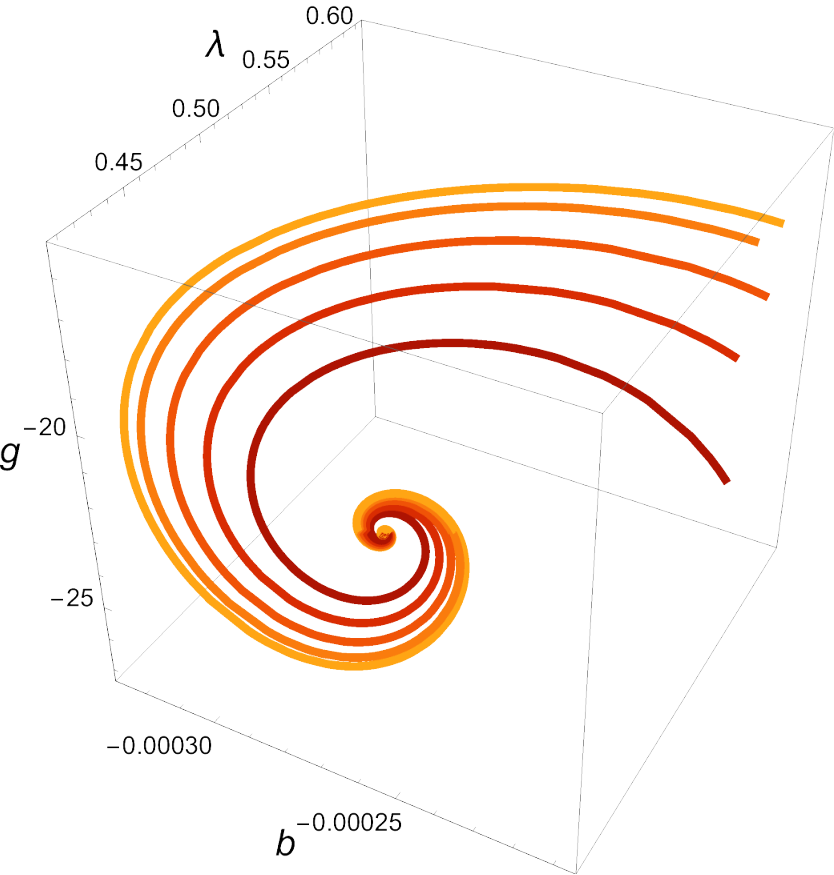
We show in Figure 1 some examples of trajectories in the 3D parameter space obtained by integrating their correspondent beta functions. Each figure depicts the attractive, spiral-like behaviour of the system around their fixed point. In particular, the figure on the left shows how the spiral behaviour flattens onto a plane when it is close to the fixed point: this is represented mathematically by the purely real, negative critical exponent λ1\lambda_{1} which contributes to the attractiveness of the fixed point, while λ2,3=θ′±i​θ′′\lambda_{2,3}=\theta^{\prime}\pm i\theta^{\prime\prime} describe the attractive spiral motion component onto a 2D plane.

Refer to caption
Refer to caption
Refer to caption
Figure 1: Flow of gg, λ\lambda and bb for various values of the cutoff.

While the present analysis was able to show the existence of a UV attractive fixed point for the quadratically truncated theory, we also wish to compare our results with the ones of of Lauscher and Reuter 2002, where a similar study was conducted taking into account all the tensorial degrees of freedom of the metric and leading, similarly, to the identification of an attractive fixed point. While this main feature once again seems to be related purely to the conformal degree of the metric, we also wish to study in depth the details of the newfound fixed point through its parameters shown in Tables 2-4. Before doing this, we also notice that while in the pure CREH model the UV-attractive non-Gaussian fixed point coexisted with the usual Gaussian fixed point (g∗,λ∗)=(0,0)(g^{*},\lambda^{*})=(0,0), characterized by both an attractive and repulsive direction, in this new model the Gaussian fixed point is lost: (g,λ,b)=(0,0,0)(g,\lambda,b)=(0,0,0) is a fixed point solution only for the beta functions ∂tgk\partial_{t}g_{k} and ∂tλk\partial_{t}\lambda_{k}. This is in line with the results of Lauscher and Reuter 2002, where a Gaussian fixed point does not appear. Regarding the parameters in Tables 2-4, we show in Figure 2 the plots of the resulting critical exponents at different values of nn. In order to perform a clear comparison with Lauscher and Reuter 2002, we have renamed θ3≔−λ1{\theta_{3}\coloneqq-\lambda_{1}} and −λ2,3≔θ′±i​θ′′{-\lambda_{2,3}\coloneqq\theta^{\prime}\pm i\theta^{\prime\prime}} to work with positive quantities. Figure 3 contains similar plots for the coordinate values of b∗b^{*} and the product b∗​g∗​λ∗b^{*}g^{*}\lambda^{*}, where the rotation (g∗,λ∗,b∗)→(−g∗,λ∗,−b∗)(g^{*},\lambda^{*},b^{*})\to(-g^{*},\lambda^{*},-b^{*}) was performed for the same reason. As the quantities described in Figures 2-3 do not change switching cutoff family, such plots are represented for only one regularizator shape ρk2​(s,n)\rho_{k}^{2}(s,n). Figure 4 contains instead plots regarding the behaviour of the coordinates g∗g^{*}, λ∗\lambda^{*} and product g∗​λ∗g^{*}\lambda^{*}. As the coordinates g∗g^{*} and λ∗\lambda^{*} depend on the regularizator shape applied, we represent the plot for each cutoff family .

Figure 2: Plot of the critical exponents λ1\lambda_{1}, θ′\theta^{\prime} and θ′′\theta^{\prime\prime} for different values of nn. Second cutoff family ρk2​(s,n)\rho^{2}_{k}(s,n) implemented.
Figure 3: Plot of the fixed point coordinate b∗b^{*} and the product b∗​g∗​λ∗b^{*}g^{*}\lambda^{*} for different values of nn. Second cutoff family ρk2​(s,n)\rho^{2}_{k}(s,n) implemented.
Figure 4: Plot of the fixed point coordinates g∗g^{*}, λ∗\lambda^{*} and the product g∗​λ∗g^{*}\lambda^{*} for different values of nn. First cutoff family ρk1​(s,n)\rho^{1}_{k}(s,n) implemented on the left figure, second cutoff family ρk2​(s,n)\rho^{2}_{k}(s,n) implemented on the right figure.

The curve describing the critical exponents closely resembles the behaviour found by Lauscher and Reuter 2002 when implementing a family of exponential shape functions as regulators (see Figure 6 of Lauscher and Reuter 2002). On top of this, the new critical exponent θ3\theta_{3} is of bigger order of magnitude with respect to the other exponents, exactly as in Lauscher and Reuter 2002. The curve for b∗b^{*} and the coordinates g∗g^{*}, λ∗\lambda^{*} and g∗​λ∗g^{*}\lambda^{*} also share similar behaviours as in Figure 3 of Lauscher and Reuter 2002, further highlighting the many similarities of the two studies, in spite of the big difference in the difficulty of the problems tackled. The only clear difference between the purely conformal theory results and the full degrees of freedom problem is shown in the right panel of Figure 4, where the behaviour of g∗g^{*} decreases with nn instead of increasing. As we already determined that the universal quantities emerging from this analysis are the critical exponents, together with g∗​λ∗g^{*}\lambda^{*}, g∗​λ∗​b∗g^{*}\lambda^{*}b^{*} and b∗b^{*}, it does not surprise us that these are the quantities which can safely be compared between different pictures of the same model, such as this analysis and the one already performed in Lauscher and Reuter 2002. While strictly focusing on these parameters, the behaviours in both results share many similarities: this once again suggests that the conformal component of the metric is truly able to capture a significant portion of the UV behaviour of the model.

V Conclusions

In this work we have shown that the critical properties Reuter fixed point of a conformally reduced quadratic gravity theory like R+R2R+R^{2} are determined by the dynamics of the conformal factor. Our approach is closer in spirit to the original paper by Reuter and Lauscher Lauscher and Reuter 2002 it employs a linear parametrisation of the fluctuations and a compact topology for the projection of the flow equation. The role of the additional propagating degrees of freedom, if we compare our result with the full calculation presented in Lauscher and Reuter 2002 is essentially confined to the location of the fixed point in the theory space. On the contrary the behavior and the stability of the critical exponents against change in the regulator is qualitatively very similar to that of the full theory. It would be very important to consider higher truncation in the CREH approximation to see if the critical properties of the theory are still determined by the conformal factor. In fact this would have far reaching consequences for the structure of the vacuum of the full theory which could be dominated by non-homogeneous field configuration which dominated the path integral as showed in Bonanno and Reuter 2013. Moreover it could also shed light in a proper definition of the cutoff for the general f⁡(R)f(R) theory for which the definition of a global scaling solution strongly depend on the details of the chosen regulator Morris and Stulga 2022. We hope to return on these points in a following work.

Acknowledgements

AB and MC would like to thank Benjamin Knorr for important comments and suggestions on an earlier version of the manuscript. MC would like to thank the National Institute of Astrophysics (INAF) section of Catania and the INAF- Catania Astrophysical Observatory for warm hospitality during the preparation of the manuscript. MC acknowledges support from INFN.

Appendix A Fixed point parameter tables

Fixed point parameters for ρk1​(s,n)\rho_{k}^{1}(s,n), β→0\beta\to 0 Fixed point parameters for ρk2​(s,n)\rho_{k}^{2}(s,n), β→0\beta\to 0
𝐧\mathbf{n} 𝐳∗\mathbf{z^{*}} 𝐠∗\mathbf{g^{*}} λ∗\mathbf{\lambda^{*}} 𝐠∗​λ∗\mathbf{g^{*}\lambda^{*}} θ′\mathbf{\theta^{\prime}} θ′′\mathbf{\theta^{\prime\prime}} 𝐧\mathbf{n} 𝐳∗\mathbf{z^{*}} 𝐠∗\mathbf{g^{*}} λ∗\mathbf{\lambda^{*}} 𝐠∗​λ∗\mathbf{g^{*}\lambda^{*}} θ′\mathbf{\theta^{\prime}} θ′′\mathbf{\theta^{\prime\prime}}
𝟑\mathbf{3} −0.050-0.050 4.7124.712 0.3750.375 1.7671.767 −3.000-3.000 4.7954.795 𝟑\mathbf{3} −0.151-0.151 1.5701.570 1.1251.125 1.7671.767 −3.000-3.000 4.7954.795
𝟓\mathbf{5} −0.025-0.025 9.4249.424 0.2500.250 2.3562.356 −1.000-1.000 3.8723.872 𝟓\mathbf{5} −0.126-0.126 1.8841.884 1.2501.250 2.3562.356 −1.000-1.000 3.8723.872
𝟕\mathbf{7} −0.017-0.017 13.48213.482 0.1870.187 2.5272.527 −0.600-0.600 3.5273.527 𝟕\mathbf{7} −0.123-0.123 1.9261.926 1.3121.312 2.5272.527 −0.600-0.600 3.5273.527
𝟗\mathbf{9} −0.013-0.013 17.38617.386 0.1500.150 2.6072.607 −0.428-0.428 3.3533.353 𝟗\mathbf{9} −0.123-0.123 1.9311.931 1.3501.350 2.6072.607 −0.428-0.428 3.3533.353
+∞\mathbf{+\infty} −- −- −- −- −- −- +∞\mathbf{+\infty} −0.127-0.127 1.8761.876 1.5001.500 2.8152.815 00 2.8282.828
Table 1: Fixed point parameters obtained using the first cutoff ρk1​(s,n)\rho_{k}^{1}(s,n) (on the left) and the second cutoff ρk2​(s,n)\rho_{k}^{2}(s,n) (on the right) in the pure CREH limit case β→0\beta\to 0.
Fixed point parameters for ρk1​(s,n)\rho_{k}^{1}(s,n) Fixed point parameters for ρk2​(s,n)\rho_{k}^{2}(s,n)
𝐧\mathbf{n} 𝐳∗\mathbf{z^{*}} 𝐠∗\mathbf{g^{*}} λ∗\mathbf{\lambda^{*}} 𝐛∗\mathbf{b^{*}} 𝐧\mathbf{n} 𝐳∗\mathbf{z^{*}} 𝐠∗\mathbf{g^{*}} λ∗\mathbf{\lambda^{*}} 𝐛∗\mathbf{b^{*}}
𝟑\mathbf{3} 3.276×10−33.276\times 10^{-3} −72.870-72.870 0.1690.169 −3.695×10⁻⁴-3.695\times 10^{-4} 𝟑\mathbf{3} 9.828×10−39.828\times 10^{-3} −24.290-24.290 0.5090.509 −3.695×10⁻⁴-3.695\times 10^{-4}
𝟓\mathbf{5} 2.027×10−32.027\times 10^{-3} −117.731-117.731 0.0990.099 −3.223×10⁻⁴-3.223\times 10^{-4} 𝟓\mathbf{5} 1.013×10−21.013\times 10^{-2} −23.546-23.546 0.4960.496 −3.223×10⁻⁴-3.223\times 10^{-4}
𝟕\mathbf{7} 1.460×10−31.460\times 10^{-3} −163.484-163.484 0.0690.069 −3.061×10⁻⁴-3.061\times 10^{-4} 𝟕\mathbf{7} 1.022×10−21.022\times 10^{-2} −23.354-23.354 0.4880.488 −3.061×10⁻⁴-3.061\times 10^{-4}
𝟗\mathbf{9} 1.139×10−31.139\times 10^{-3} −209.495-209.495 0.0530.053 −2.979×10⁻⁴-2.979\times 10^{-4} 𝟗\mathbf{9} 1.025×10−21.025\times 10^{-2} −23.277-23.277 0.4840.484 −2.979×10⁻⁴-2.979\times 10^{-4}
𝟏𝟎\mathbf{10} 1.026×10−31.026\times 10^{-3} −232.547-232.547 0.0480.048 −2.951×10⁻⁴-2.951\times 10^{-4} 𝟏𝟎\mathbf{10} 1.026×10−21.026\times 10^{-2} −23.254-23.254 0.4820.482 −2.951×10⁻⁴-2.951\times 10^{-4}
𝟏𝟓\mathbf{15} 6.859×10−46.859\times 10^{-4} −348.009-348.009 0.0310.031 −2.872×10⁻⁴-2.872\times 10^{-4} 𝟏𝟓\mathbf{15} 1.028×10−21.028\times 10^{-2} −23.200-23.200 0.4780.478 −2.872×10⁻⁴-2.872\times 10^{-4}
𝟐𝟎\mathbf{20} 5.149×10−45.149\times 10^{-4} −463.619-463.619 0.0230.023 −2.835×10⁻⁴-2.835\times 10^{-4} 𝟐𝟎\mathbf{20} 1.029×10−21.029\times 10^{-2} −23.180-23.180 0.4750.475 −2.835×10⁻⁴-2.835\times 10^{-4}
𝟑𝟎\mathbf{30} 3.435×10−43.435\times 10^{-4} −694.983-694.983 0.0150.015 −2.798×10⁻⁴-2.798\times 10^{-4} 𝟑𝟎\mathbf{30} 1.030×10−21.030\times 10^{-2} −23.166-23.166 0.4720.472 −2.798×10⁻⁴-2.798\times 10^{-4}
𝟒𝟎\mathbf{40} 2.576×10−42.576\times 10^{-4} −926.417-926.417 0.0110.011 −2.781×10⁻⁴-2.781\times 10^{-4} 𝟒𝟎\mathbf{40} 1.030×10−21.030\times 10^{-2} −23.160-23.160 0.4710.471 −2.781×10⁻⁴-2.781\times 10^{-4}
𝟓𝟎\mathbf{50} 2.061×10−42.061\times 10^{-4} −1157.879-1157.879 0.0090.009 −2.770×10⁻⁴-2.770\times 10^{-4} 𝟓𝟎\mathbf{50} 1.030×10−21.030\times 10^{-2} −23.157-23.157 0.4700.470 −2.770×10⁻⁴-2.770\times 10^{-4}
+∞\mathbf{+\infty} −- −- −- −- +∞\mathbf{+\infty} 1.031×10−21.031\times 10^{-2} −23.150-23.150 0.4670.467 −2.729×10⁻⁴-2.729\times 10^{-4}
Table 2: Fixed point parameters obtained using the first cutoff ρk1​(s,n)\rho_{k}^{1}(s,n) (on the left) and the second cutoff ρk2​(s,n)\rho_{k}^{2}(s,n) (on the right) in the quadratic theory.
Fixed point parameters for ρk1​(s,n)\rho_{k}^{1}(s,n) Fixed point parameters for ρk2​(s,n)\rho_{k}^{2}(s,n)
𝐧\mathbf{n} 𝐠∗​λ∗\mathbf{g^{*}\lambda^{*}} 𝐛∗​λ∗\mathbf{b^{*}\lambda^{*}} 𝐛∗​𝐠∗\mathbf{b^{*}g^{*}} 𝐛∗​𝐠∗​λ∗\mathbf{b^{*}g^{*}\lambda^{*}} 𝐧\mathbf{n} 𝐠∗​λ∗\mathbf{g^{*}\lambda^{*}} 𝐛∗​λ∗\mathbf{b^{*}\lambda^{*}} 𝐛∗​𝐠∗\mathbf{b^{*}g^{*}} 𝐛∗​𝐠∗​λ∗\mathbf{b^{*}g^{*}\lambda^{*}}
𝟑\mathbf{3} −12.382-12.382 −6.279×10⁻⁵-6.279\times 10^{-5} 0.0260.026 4.575×10−34.575\times 10^{-3} 𝟑\mathbf{3} −12.382-12.382 −1.883×10⁻⁴-1.883\times 10^{-4} 8.975×10−38.975\times 10^{-3} 4.575×10−34.575\times 10^{-3}
𝟓\mathbf{5} −11.682-11.682 −3.198×10⁻⁵-3.198\times 10^{-5} 0.0370.037 3.765×10−33.765\times 10^{-3} 𝟓\mathbf{5} −11.682-11.682 −1.599×10⁻⁴-1.599\times 10^{-4} 7.589×10−37.589\times 10^{-3} 3.765×10−33.765\times 10^{-3}
𝟕\mathbf{7} −11.418-11.418 −2.138×10⁻⁵-2.138\times 10^{-5} 0.0500.050 3.495×10−33.495\times 10^{-3} 𝟕\mathbf{7} −11.418-11.418 −1.496×10⁻⁴-1.496\times 10^{-4} 7.149×10−37.149\times 10^{-3} 3.495×10−33.495\times 10^{-3}
𝟗\mathbf{9} −11.279-11.279 −1.604×10⁻⁵-1.604\times 10^{-5} 0.0620.062 3.360×10−33.360\times 10^{-3} 𝟗\mathbf{9} −11.279-11.279 −1.443×10⁻⁴-1.443\times 10^{-4} 6.934×10−36.934\times 10^{-3} 3.360×10−33.360\times 10^{-3}
𝟏𝟎\mathbf{10} −11.231-11.231 −1.425×10⁻⁵-1.425\times 10^{-5} 0.0680.068 3.315×10−33.315\times 10^{-3} 𝟏𝟎\mathbf{10} −11.231-11.231 −1.425×10⁻⁴-1.425\times 10^{-4} 6.864×10−36.864\times 10^{-3} 3.315×10−33.315\times 10^{-3}
𝟏𝟓\mathbf{15} −11.092-11.092 −9.156×10⁻⁶-9.156\times 10^{-6} 0.0990.099 3.186×10−33.186\times 10^{-3} 𝟏𝟓\mathbf{15} −11.092-11.092 −1.373×10⁻⁴-1.373\times 10^{-4} 6.665×10−36.665\times 10^{-3} 3.186×10−33.186\times 10^{-3}
𝟐𝟎\mathbf{20} −11.024-11.024 −6.741×10⁻⁶-6.741\times 10^{-6} 0.1310.131 3.125×10−33.125\times 10^{-3} 𝟐𝟎\mathbf{20} −11.024-11.024 −1.348×10⁻⁴-1.348\times 10^{-4} 6.572×10−36.572\times 10^{-3} 3.125×10−33.125\times 10^{-3}
𝟑𝟎\mathbf{30} −10.957-10.957 −4.412×10⁻⁶-4.412\times 10^{-6} 0.1940.194 3.066×10−33.066\times 10^{-3} 𝟑𝟎\mathbf{30} −10.957-10.957 −1.323×10⁻⁴-1.323\times 10^{-4} 6.483×10−36.483\times 10^{-3} 3.066×10−33.066\times 10^{-3}
𝟒𝟎\mathbf{40} −10.924-10.924 −3.279×10⁻⁶-3.279\times 10^{-6} 0.2570.257 3.038×10−33.038\times 10^{-3} 𝟒𝟎\mathbf{40} −10.924-10.924 −1.311×10⁻⁴-1.311\times 10^{-4} 6.441×10−36.441\times 10^{-3} 3.038×10−33.038\times 10^{-3}
𝟓𝟎\mathbf{50} −10.904-10.904 −2.609×10⁻⁶-2.609\times 10^{-6} 0.3200.320 3.021×10−33.021\times 10^{-3} 𝟓𝟎\mathbf{50} −10.904-10.904 −1.304×10⁻⁴-1.304\times 10^{-4} 6.415×10−36.415\times 10^{-3} 3.021×10−33.021\times 10^{-3}
+∞\mathbf{+\infty} −- −- −- −- +∞\mathbf{+\infty} −10.826-10.826 −1.276×10⁻⁴-1.276\times 10^{-4} 6.318×10−36.318\times 10^{-3} 2.954×10−32.954\times 10^{-3}
Table 3: Fixed point parameters obtained using the first cutoff ρk1​(s,n)\rho_{k}^{1}(s,n) (on the left) and the second cutoff ρk2​(s,n)\rho_{k}^{2}(s,n) (on the right) in the quadratic theory.
Fixed point parameters for ρk1​(s,n)\rho_{k}^{1}(s,n) Fixed point parameters for ρk2​(s,n)\rho_{k}^{2}(s,n)
𝐧\mathbf{n} λ𝟏\mathbf{\lambda_{1}} θ′\mathbf{\theta^{\prime}} θ′′\mathbf{\theta^{\prime\prime}} 𝐧\mathbf{n} λ𝟏\mathbf{\lambda_{1}} θ′\mathbf{\theta^{\prime}} θ′′\mathbf{\theta^{\prime\prime}}
𝟑\mathbf{3} −3.035-3.035 −0.584-0.584 1.4881.488 𝟑\mathbf{3} −3.035-3.035 −0.584-0.584 1.4881.488
𝟓\mathbf{5} −2.546-2.546 −0.586-0.586 1.4941.494 𝟓\mathbf{5} −2.546-2.546 −0.586-0.586 1.4941.494
𝟕\mathbf{7} −2.382-2.382 −0.588-0.588 1.5001.500 𝟕\mathbf{7} −2.382-2.382 −0.588-0.588 1.5001.500
𝟗\mathbf{9} −2.300-2.300 −0.589-0.589 1.5041.504 𝟗\mathbf{9} −2.300-2.300 −0.589-0.589 1.5041.504
𝟏𝟎\mathbf{10} −2.272-2.272 −0.589-0.589 1.5051.505 𝟏𝟎\mathbf{10} −2.272-2.272 −0.589-0.589 1.5051.505
𝟏𝟓\mathbf{15} −2.193-2.193 −0.590-0.590 1.5101.510 𝟏𝟓\mathbf{15} −2.193-2.193 −0.590-0.590 1.5101.510
𝟐𝟎\mathbf{20} −2.156-2.156 −0.591-0.591 1.5121.512 𝟐𝟎\mathbf{20} −2.156-2.156 −0.591-0.591 1.5121.512
𝟑𝟎\mathbf{30} −2.120-2.120 −0.592-0.592 1.5151.515 𝟑𝟎\mathbf{30} −2.120-2.120 −0.592-0.592 1.5151.515
𝟒𝟎\mathbf{40} −2.103-2.103 −0.592-0.592 1.5161.516 𝟒𝟎\mathbf{40} −2.103-2.103 −0.592-0.592 1.5161.516
𝟓𝟎\mathbf{50} −2.092-2.092 −0.592-0.592 1.5171.517 𝟓𝟎\mathbf{50} −2.092-2.092 −0.592-0.592 1.5171.517
+∞\mathbf{+\infty} −- −- −- +∞\mathbf{+\infty} −2.503-2.503 −0.709-0.709 1.9661.966
Table 4: Fixed point parameters obtained using the first cutoff ρk1​(s,n)\rho_{k}^{1}(s,n) (on the left) and the second cutoff ρk2​(s,n)\rho_{k}^{2}(s,n) (on the right) in the quadratic theory.

Appendix B Explicit expressions for beta functions

In this section, we explicitly report some explicit expressions for the beta functions obtained for dimension d=4d=4 using the second cutoff ρk2​(s,n)\rho_{k}^{2}(s,n) at different values for the smoothness parameter nn (finite n={3,5,7,9}n=\left\{3,5,7,9\right\} and the limit n→∞n\to\infty). We do not show the remaining n={10,15,20,30,40,50}n=\left\{10,15,20,30,40,50\right\} as their expressions get extremely cumbersome. Each choice of nn leads to couples of beta functions depending on the sign of the coupling β\beta. This section contains beta functions only related to the sign β<0\beta<0, which are the ones leading to significant physical results as shown in Section IV. Beta functions for β>0\beta>0 are not shown here due to excessive length. To avoid further prolixity, we do not include the explicit expressions for the beta functions pertaining the choice of the first cutoff ρk1​(s,n)\rho_{k}^{1}(s,n), as they share similar structure to their second cutoff counterparts.

B.0.1 Beta functions for dimensionless couplings at d=4d=4, with second cutoff ρk2​(s,n)\rho_{k}^{2}(s,n), smoothness parameter n=3n=3

∂tz=−116​π2​(3−2​λ)2​(288​b​(2​λ−3)+z)4​(220150628352​π2​b4​(3−2​λ)6​z+z4​(32​π2​(3−2​λ)2​z+27)+CLOSE\displaystyle\partial_{t}z=-\frac{1}{16\pi^{2}(3-2\lambda)^{2}(288b(2\lambda-3)+z)^{4}}\left(220150628352\pi^{2}b^{4}(3-2\lambda)^{6}z+z^{4}\left(32\pi^{2}(3-2\lambda)^{2}z+27\right)+\right.
+144​b​(2​λ−3)​z3​(256​π2​(3−2​λ)2​z+351)+\displaystyle+144b(2\lambda-3)z^{3}\left(256\pi^{2}(3-2\lambda)^{2}z+351\right)+
+5971968​b3​(2​λ−3)3​z​(−81​π​288​b​(3−2​λ)−z+512​π2​(3−2​λ)2​z3/2−1134​z)+\displaystyle+5971968b^{3}(2\lambda-3)^{3}\sqrt{z}\left(-81\pi\sqrt{288b(3-2\lambda)-z}+512\pi^{2}(3-2\lambda)^{2}z^{3/2}-1134\sqrt{z}\right)+
+62208​b2​(3−2​λ)2​z3/2​(243​π​288​b​(3−2​λ)−z+256​π2​(3−2​λ)2​z3/2−180​z)+\displaystyle+62208b^{2}(3-2\lambda)^{2}z^{3/2}\left(243\pi\sqrt{288b(3-2\lambda)-z}+256\pi^{2}(3-2\lambda)^{2}z^{3/2}-180\sqrt{z}\right)+
OPEN−30233088​b2​(3−2​λ)2​z​(32​b​(2​λ−3)−z)​288​b​(2​λ−3)+z​tanh−1⁡(z288​b​(2​λ−3)+z))\displaystyle\left.-30233088b^{2}(3-2\lambda)^{2}\sqrt{z}(32b(2\lambda-3)-z)\sqrt{288b(2\lambda-3)+z}\tanh^{-1}\left(\frac{\sqrt{z}}{\sqrt{288b(2\lambda-3)+z}}\right)\right)
∂tλ=116​π2​(3−2​λ)2​z​(288​b​(2​λ−3)+z)4​(z7/2​(λ⁡(189−32​π2​(3−2​λ)2​z)−243)−220150628352​π2​b4​(3−2​λ)6​λ​z+CLOSE\displaystyle\partial_{t}\lambda=\frac{1}{16\pi^{2}(3-2\lambda)^{2}\sqrt{z}(288b(2\lambda-3)+z)^{4}}\left(z^{7/2}\left(\lambda\left(189-32\pi^{2}(3-2\lambda)^{2}z\right)-243\right)-220150628352\pi^{2}b^{4}(3-2\lambda)^{6}\lambda\sqrt{z}+\right.
−5971968​b3​(2​λ−3)3​(81​π​λ​288​b​(3−2​λ)−z+512​π2​λ​(3−2​λ)2​z3/2+486​(5​λ−4)​z)+\displaystyle-5971968b^{3}(2\lambda-3)^{3}\left(81\pi\lambda\sqrt{288b(3-2\lambda)-z}+512\pi^{2}\lambda(3-2\lambda)^{2}z^{3/2}+486(5\lambda-4)\sqrt{z}\right)+
+144​b​(2​λ−3)​z2​(243​π​(2​λ−3)​288​b​(3−2​λ)−z−256​π2​λ​(3−2​λ)2​z3/2+351​λ​z)+\displaystyle+144b(2\lambda-3)z^{2}\left(243\pi(2\lambda-3)\sqrt{288b(3-2\lambda)-z}-256\pi^{2}\lambda(3-2\lambda)^{2}z^{3/2}+351\lambda\sqrt{z}\right)+
−62208​b2​(3−2​λ)2​z​(−81​π​(7​λ−6)​288​b​(3−2​λ)−z+256​π2​λ​(3−2​λ)2​z3/2+36​(23​λ−27)​z)+\displaystyle-62208b^{2}(3-2\lambda)^{2}z\left(-81\pi(7\lambda-6)\sqrt{288b(3-2\lambda)-z}+256\pi^{2}\lambda(3-2\lambda)^{2}z^{3/2}+36(23\lambda-27)\sqrt{z}\right)+
OPEN−69984​b​(3−2​λ)2​288​b​(2​λ−3)+z​(13824​b2​λ​(2​λ−3)+144​b​(6−7​λ)​z−z2)​tanh−1⁡(z288​b​(2​λ−3)+z))\displaystyle\left.-69984b(3-2\lambda)^{2}\sqrt{288b(2\lambda-3)+z}\left(13824b^{2}\lambda(2\lambda-3)+144b(6-7\lambda)z-z^{2}\right)\tanh^{-1}\left(\frac{\sqrt{z}}{\sqrt{288b(2\lambda-3)+z}}\right)\right)
∂tb=−3256​π2​(288​b​(2​λ−3)+z)5​(3962711310336​b5​(3−2​λ)2+2021760​b2​z32​λ−3+1944​b​z4(3−2​λ)2+z5(2​λ−3)3+CLOSE\displaystyle\partial_{t}b=-\frac{3}{256\pi^{2}(288b(2\lambda-3)+z)^{5}}\left(3962711310336b^{5}(3-2\lambda)^{2}+\frac{2021760b^{2}z^{3}}{2\lambda-3}+\frac{1944bz^{4}}{(3-2\lambda)^{2}}+\frac{z^{5}}{(2\lambda-3)^{3}}+\right.
−4478976​b3​z3/2​(96​z−115​π​288​b​(3−2​λ)−z)−429981696​b4​(2​λ−3)​(75​π​z​288​b​(3−2​λ)−z+554​z)+\displaystyle-4478976b^{3}z^{3/2}\left(96\sqrt{z}-115\pi\sqrt{288b(3-2\lambda)-z}\right)-429981696b^{4}(2\lambda-3)\left(75\pi\sqrt{z}\sqrt{288b(3-2\lambda)-z}+554z\right)+
OPEN+44789760​b3​z​(23​z−1440​b​(2​λ−3))​288​b​(2​λ−3)+z​tanh−1⁡(z288​b​(2​λ−3)+z))\displaystyle\left.+44789760b^{3}\sqrt{z}(23z-1440b(2\lambda-3))\sqrt{288b(2\lambda-3)+z}\tanh^{-1}\left(\frac{\sqrt{z}}{\sqrt{288b(2\lambda-3)+z}}\right)\right)

B.0.2 Beta functions for dimensionless couplings at d=4d=4, with second cutoff ρk2​(s,n)\rho_{k}^{2}(s,n), smoothness parameter n=5n=5

∂tz=−132​π2​(5−2​λ)4​(288​b​(2​λ−5)+z)6​(z6​(64​π2​(5−2​λ)4​z+3125)+CLOSE\displaystyle\partial_{t}z=-\frac{1}{32\pi^{2}(5-2\lambda)^{4}(288b(2\lambda-5)+z)^{6}}\left(z^{6}\left(64\pi^{2}(5-2\lambda)^{4}z+3125\right)+\right.
+51840​b2​(5−2​λ)2​z4​(1536​π2​(5−2​λ)4​z+105625)+36520347436056576​π2​b6​(5−2​λ)10​z+\displaystyle+51840b^{2}(5-2\lambda)^{2}z^{4}\left(1536\pi^{2}(5-2\lambda)^{4}z+105625\right)+36520347436056576\pi^{2}b^{6}(5-2\lambda)^{10}z+
+7464960​b3​(2​λ−5)3​z3​(4096​π2​(5−2​λ)4​z+433125)+48​b​(2​λ−5)​z5​(2304​π2​(5−2​λ)4​z+128125)+\displaystyle+7464960b^{3}(2\lambda-5)^{3}z^{3}\left(4096\pi^{2}(5-2\lambda)^{4}z+433125\right)+48b(2\lambda-5)z^{5}\left(2304\pi^{2}(5-2\lambda)^{4}z+128125\right)+
+61917364224​b5​(2​λ−5)5​z​(−109375​π​288​b​(5−2​λ)−z+12288​π2​(5−2​λ)4​z3/2−2181250​z)+\displaystyle+61917364224b^{5}(2\lambda-5)^{5}\sqrt{z}\left(-109375\pi\sqrt{288b(5-2\lambda)-z}+12288\pi^{2}(5-2\lambda)^{4}z^{3/2}-2181250\sqrt{z}\right)+
+358318080​b4​(5−2​λ)4​z3/2​(1115625​π​288​b​(5−2​λ)−z+18432​π2​(5−2​λ)4​z3/2+372500​z)+\displaystyle+358318080b^{4}(5-2\lambda)^{4}z^{3/2}\left(1115625\pi\sqrt{288b(5-2\lambda)-z}+18432\pi^{2}(5-2\lambda)^{4}z^{3/2}+372500\sqrt{z}\right)+
OPEN−47029248000000​b4​(5−2​λ)4​z​(288​b​(2​λ−5)−17​z)​288​b​(2​λ−5)+z​tanh−1⁡(z288​b​(2​λ−5)+z))\displaystyle\left.-47029248000000b^{4}(5-2\lambda)^{4}\sqrt{z}(288b(2\lambda-5)-17z)\sqrt{288b(2\lambda-5)+z}\tanh^{-1}\left(\frac{\sqrt{z}}{\sqrt{288b(2\lambda-5)+z}}\right)\right)
∂tλ=132​π2​(5−2​λ)4​z​(288​b​(2​λ−5)+z)6​(−36520347436056576​π2​b6​(5−2​λ)10​λ​z+CLOSE\displaystyle\partial_{t}\lambda=\frac{1}{32\pi^{2}(5-2\lambda)^{4}\sqrt{z}(288b(2\lambda-5)+z)^{6}}\left(-36520347436056576\pi^{2}b^{6}(5-2\lambda)^{10}\lambda\sqrt{z}+\right.
+z11/2​(λ⁡(9375−64​π2​(5−2​λ)4​z)−15625)−24​b​(2​λ−5)​z9/2​(4​λ​(1152​π2​(5−2​λ)4​z−190625)+1265625)+\displaystyle+z^{11/2}\left(\lambda\left(9375-64\pi^{2}(5-2\lambda)^{4}z\right)-15625\right)-24b(2\lambda-5)z^{9/2}\left(4\lambda\left(1152\pi^{2}(5-2\lambda)^{4}z-190625\right)+1265625\right)+
−51840​b2​(5−2​λ)2​z7/2​(λ⁡(1536​π2​(5−2​λ)4​z−319375)+534375)+\displaystyle-51840b^{2}(5-2\lambda)^{2}z^{7/2}\left(\lambda\left(1536\pi^{2}(5-2\lambda)^{4}z-319375\right)+534375\right)+
−61917364224​b5​(2​λ−5)5​(109375​π​λ​288​b​(5−2​λ)−z+12288​π2​λ​(5−2​λ)4​z3/2+6250​(541​λ−480)​z)+\displaystyle-61917364224b^{5}(2\lambda-5)^{5}\left(109375\pi\lambda\sqrt{288b(5-2\lambda)-z}+12288\pi^{2}\lambda(5-2\lambda)^{4}z^{3/2}+6250(541\lambda-480)\sqrt{z}\right)+
−7464960​b3​(2​λ−5)3​z2​(−65625​π​(2​λ−5)​288​b​(5−2​λ)−z+4096​π2​λ​(5−2​λ)4​z3/2+625​(1640−1349​λ)​z)+\displaystyle-7464960b^{3}(2\lambda-5)^{3}z^{2}\left(-65625\pi(2\lambda-5)\sqrt{288b(5-2\lambda)-z}+4096\pi^{2}\lambda(5-2\lambda)^{4}z^{3/2}+625(1640-1349\lambda)\sqrt{z}\right)+
+358318080​b4​(5−2​λ)4​z​(65625​π​(29​λ−30)​288​b​(5−2​λ)−z−18432​π2​λ​(5−2​λ)4​z3/2+12500​(19​λ+27)​z)+\displaystyle+358318080b^{4}(5-2\lambda)^{4}z\left(65625\pi(29\lambda-30)\sqrt{288b(5-2\lambda)-z}-18432\pi^{2}\lambda(5-2\lambda)^{4}z^{3/2}+12500(19\lambda+27)\sqrt{z}\right)+
−979776000000b3(5−2λ)4288​b​(2​λ−5)+z×\displaystyle-979776000000b^{3}(5-2\lambda)^{4}\sqrt{288b(2\lambda-5)+z}\times
×(13824b2λ(2λ−5)+48b(30−29λ)z−z2)tanh−1(z288​b​(2​λ−5)+z))\displaystyle\left.\times\left(13824b^{2}\lambda(2\lambda-5)+48b(30-29\lambda)z-z^{2}\right)\tanh^{-1}\left(\frac{\sqrt{z}}{\sqrt{288b(2\lambda-5)+z}}\right)\right)
∂tb=−31252304​π2​(288​b​(2​λ−5)+z)7​(328683126924509184​b7​(5−2​λ)2+1474702848​b3​z4(5−2​λ)2+2268​b​z6(5−2​λ)4+CLOSE\displaystyle\partial_{t}b=-\frac{3125}{2304\pi^{2}(288b(2\lambda-5)+z)^{7}}\left(328683126924509184b^{7}(5-2\lambda)^{2}+\frac{1474702848b^{3}z^{4}}{(5-2\lambda)^{2}}+\frac{2268bz^{6}}{(5-2\lambda)^{4}}+\right.
+2327616​b2​z5(2​λ−5)3+731775098880​b4​z32​λ−5+7739670528​b5​z3/2​(32​z+12285​π​288​b​(5−2​λ)−z)+z7(2​λ−5)5+\displaystyle+\frac{2327616b^{2}z^{5}}{(2\lambda-5)^{3}}+\frac{731775098880b^{4}z^{3}}{2\lambda-5}+7739670528b^{5}z^{3/2}\left(32\sqrt{z}+12285\pi\sqrt{288b(5-2\lambda)-z}\right)+\frac{z^{7}}{(2\lambda-5)^{5}}+
−2229025112064​b6​(2​λ−5)​(1575​π​z​288​b​(5−2​λ)−z+16306​z)+\displaystyle-2229025112064b^{6}(2\lambda-5)\left(1575\pi\sqrt{z}\sqrt{288b(5-2\lambda)-z}+16306z\right)+
OPEN+14627977297920​b5​z​(13​z−480​b​(2​λ−5))​288​b​(2​λ−5)+z​tanh−1⁡(z288​b​(2​λ−5)+z))\displaystyle+\left.14627977297920b^{5}\sqrt{z}(13z-480b(2\lambda-5))\sqrt{288b(2\lambda-5)+z}\tanh^{-1}\left(\frac{\sqrt{z}}{\sqrt{288b(2\lambda-5)+z}}\right)\right)

B.0.3 Beta functions for dimensionless couplings at d=4d=4, with second cutoff ρk2​(s,n)\rho_{k}^{2}(s,n), smoothness parameter n=7n=7

∂tz=−1240​π2​(7−2​λ)6​(288​b​(2​λ−7)+z)8​(5​z8​(96​π2​(7−2​λ)6​z+823543)+CLOSE\displaystyle\partial_{t}z=-\frac{1}{240\pi^{2}(7-2\lambda)^{6}(288b(2\lambda-7)+z)^{8}}\left(5z^{8}\left(96\pi^{2}(7-2\lambda)^{6}z+823543\right)+\right.
+36288​b2​(7−2​λ)2​z6​(30720​π2​(7−2​λ)6​z+304357963)+\displaystyle+36288b^{2}(7-2\lambda)^{2}z^{6}\left(30720\pi^{2}(7-2\lambda)^{6}z+304357963\right)+
+376233984​b4​(7−2​λ)4​z4​(614400​π2​(7−2​λ)6​z+8405197507)+\displaystyle+376233984b^{4}(7-2\lambda)^{4}z^{4}\left(614400\pi^{2}(7-2\lambda)^{6}z+8405197507\right)+
+22718577733022074798080​π2​b8​(7−2​λ)14​z+720​b​(2​λ−7)​z7​(1536​π2​(7−2​λ)6​z+14000231)+\displaystyle+22718577733022074798080\pi^{2}b^{8}(7-2\lambda)^{14}z+720b(2\lambda-7)z^{7}\left(1536\pi^{2}(7-2\lambda)^{6}z+14000231\right)+
+15676416​b3​(2​λ−7)3​z5​(40960​π2​(7−2​λ)6​z+458713451)+\displaystyle+15676416b^{3}(2\lambda-7)^{3}z^{5}\left(40960\pi^{2}(7-2\lambda)^{6}z+458713451\right)+
+54177693696​b5​(2​λ−7)5​z3​(983040​π2​(7−2​λ)6​z+20161156183)+\displaystyle+54177693696b^{5}(2\lambda-7)^{5}z^{3}\left(983040\pi^{2}(7-2\lambda)^{6}z+20161156183\right)+
+4814694242058240​b7​(2​λ−7)7​z​(190238433​π​288​b​(7−2​λ)−z+131072​π2​(7−2​λ)6​z3/2−4679371326​z)+\displaystyle+4814694242058240b^{7}(2\lambda-7)^{7}\sqrt{z}\left(190238433\pi\sqrt{288b(7-2\lambda)-z}+131072\pi^{2}(7-2\lambda)^{6}z^{3/2}-4679371326\sqrt{z}\right)+
+39007939461120​b6​(7−2​λ)6​z3/2​(−2038268925​π​288​b​(7−2​λ)−z+196608​π2​(7−2​λ)6​z3/2+2242389940​z)+\displaystyle+39007939461120b^{6}(7-2\lambda)^{6}z^{3/2}\left(-2038268925\pi\sqrt{288b(7-2\lambda)-z}+196608\pi^{2}(7-2\lambda)^{6}z^{3/2}+2242389940\sqrt{z}\right)+
OPEN−6360693666550571335680​b6​(7−2​λ)6​z​(288​b​(2​λ−7)−25​z)​288​b​(2​λ−7)+z​tanh−1⁡(z288​b​(2​λ−7)+z))\displaystyle\left.-6360693666550571335680b^{6}(7-2\lambda)^{6}\sqrt{z}(288b(2\lambda-7)-25z)\sqrt{288b(2\lambda-7)+z}\tanh^{-1}\left(\frac{\sqrt{z}}{\sqrt{288b(2\lambda-7)+z}}\right)\right)
∂tλ=1240​π2​(7−2​λ)6​z​(288​b​(2​λ−7)+z)8​(−22718577733022074798080​π2​b8​(7−2​λ)14​λ​z+CLOSE\displaystyle\partial_{t}\lambda=\frac{1}{240\pi^{2}(7-2\lambda)^{6}\sqrt{z}(288b(2\lambda-7)+z)^{8}}\left(-22718577733022074798080\pi^{2}b^{8}(7-2\lambda)^{14}\lambda\sqrt{z}+\right.
+z15/2​(λ⁡(9058973−480​π2​(7−2​λ)6​z)−17294403)+\displaystyle+z^{15/2}\left(\lambda\left(9058973-480\pi^{2}(7-2\lambda)^{6}z\right)-17294403\right)+
−7838208​b3​(2​λ−7)3​z9/2​(20​λ​(4096​π2​(7−2​λ)6​z−98236915)+3665589893)+\displaystyle-7838208b^{3}(2\lambda-7)^{3}z^{9/2}\left(20\lambda\left(4096\pi^{2}(7-2\lambda)^{6}z-98236915\right)+3665589893\right)+
−36​b​(2​λ−7)​z13/2​(2​λ​(15360​π2​(7−2​λ)6​z−305534453)+1158725001)+\displaystyle-36b(2\lambda-7)z^{13/2}\left(2\lambda\left(15360\pi^{2}(7-2\lambda)^{6}z-305534453\right)+1158725001\right)+
−36288​b2​(7−2​λ)2​z11/2​(λ⁡(30720​π2​(7−2​λ)6​z−658010857)+1237785129)+\displaystyle-36288b^{2}(7-2\lambda)^{2}z^{11/2}\left(\lambda\left(30720\pi^{2}(7-2\lambda)^{6}z-658010857\right)+1237785129\right)+
−376233984​b4​(7−2​λ)4​z7/2​(λ⁡(614400​π2​(7−2​λ)6​z−18035709349)+33706791447)+\displaystyle-376233984b^{4}(7-2\lambda)^{4}z^{7/2}\left(\lambda\left(614400\pi^{2}(7-2\lambda)^{6}z-18035709349\right)+33706791447\right)+
+4814694242058240​b7​(7−2​λ)7​(131072​π2​λ​(7−2​λ)6​z3/2+1647086​(3865​λ−3584)​z)+\displaystyle+4814694242058240b^{7}(7-2\lambda)^{7}\left(131072\pi^{2}\lambda(7-2\lambda)^{6}z^{3/2}+1647086(3865\lambda-3584)\sqrt{z}\right)+
−915939887983282272337920​π​b7​(7−2​λ)7​λ​288​b​(7−2​λ)−z+\displaystyle-915939887983282272337920\pi b^{7}(7-2\lambda)^{7}\lambda\sqrt{288b(7-2\lambda)-z}+
−54177693696​b5​(2​λ−7)5​z2​(983040​π2​(7−2​λ)6​λ​z3/2−117649​(300247​λ−451080)​z)+\displaystyle-54177693696b^{5}(2\lambda-7)^{5}z^{2}\left(983040\pi^{2}(7-2\lambda)^{6}\lambda z^{3/2}-117649(300247\lambda-451080)\sqrt{z}\right)+
−66257225693235118080​π​b5​(2​λ−7)6​z2​288​b​(7−2​λ)−z+\displaystyle-66257225693235118080\pi b^{5}(2\lambda-7)^{6}z^{2}\sqrt{288b(7-2\lambda)-z}+
−39007939461120​b6​(7−2​λ)6​z​(196608​π2​(7−2​λ)6​λ​z3/2−470596​(6751​λ−6951)​z)+\displaystyle-39007939461120b^{6}(7-2\lambda)^{6}z\left(196608\pi^{2}(7-2\lambda)^{6}\lambda z^{3/2}-470596(6751\lambda-6951)\sqrt{z}\right)+
−3180346833275285667840​π​b6​(7−2​λ)6​(37​λ−42)​z​288​b​(7−2​λ)−z+\displaystyle-3180346833275285667840\pi b^{6}(7-2\lambda)^{6}(37\lambda-42)z\sqrt{288b(7-2\lambda)-z}+
−132514451386470236160b5(7−2λ)6288​b​(2​λ−7)+z×\displaystyle-132514451386470236160b^{5}(7-2\lambda)^{6}\sqrt{288b(2\lambda-7)+z}\times
×(13824b2λ(2λ−7)+48b(42−37λ)z−z2)tanh−1(z288​b​(2​λ−7)+z))\displaystyle\left.\times\left(13824b^{2}\lambda(2\lambda-7)+48b(42-37\lambda)z-z^{2}\right)\tanh^{-1}\left(\frac{\sqrt{z}}{\sqrt{288b(2\lambda-7)+z}}\right)\right)
∂tb=−8235432304​π2​(288​b​(2​λ−7)+z)9​(2597432832​b3​z6(7−2​λ)4+496573391241216​b5​z4(7−2​λ)2+2760​b​z8(7−2​λ)6+CLOSE\displaystyle\partial_{t}b=-\frac{823543}{2304\pi^{2}(288b(2\lambda-7)+z)^{9}}\left(\frac{2597432832b^{3}z^{6}}{(7-2\lambda)^{4}}+\frac{496573391241216b^{5}z^{4}}{(7-2\lambda)^{2}}+\frac{2760bz^{8}}{(7-2\lambda)^{6}}+\right.
+27262293279626489757696​b9​(7−2​λ)2+1322964099072​b4​z5(2​λ−7)3+3452544​b2​z7(2​λ−7)5+z9(2​λ−7)7+\displaystyle+27262293279626489757696b^{9}(7-2\lambda)^{2}+\frac{1322964099072b^{4}z^{5}}{(2\lambda-7)^{3}}+\frac{3452544b^{2}z^{7}}{(2\lambda-7)^{5}}+\frac{z^{9}}{(2\lambda-7)^{7}}+
+159936452584538112​b6​z32​λ−7+69331597085638656​b8​(2​λ−7)​z​(5005​π​288​b​(7−2​λ)−z−63718​z)+\displaystyle+\frac{159936452584538112b^{6}z^{3}}{2\lambda-7}+69331597085638656b^{8}(2\lambda-7)\sqrt{z}\left(5005\pi\sqrt{288b(7-2\lambda)-z}-63718\sqrt{z}\right)+
+26748301344768​b7​(312896​z2−495495​π​z3/2​288​b​(7−2​λ)−z)+\displaystyle+26748301344768b^{7}\left(312896z^{2}-495495\pi z^{3/2}\sqrt{288b(7-2\lambda)-z}\right)+
OPEN−2409754468150149120​b7​z​(288​b​(2​λ−7)−11​z)​288​b​(2​λ−7)+z​tanh−1⁡(z288​b​(2​λ−7)+z))\displaystyle\left.-2409754468150149120b^{7}\sqrt{z}(288b(2\lambda-7)-11z)\sqrt{288b(2\lambda-7)+z}\tanh^{-1}\left(\frac{\sqrt{z}}{\sqrt{288b(2\lambda-7)+z}}\right)\right)

B.0.4 Beta functions for dimensionless couplings at d=4d=4, with second cutoff ρk2​(s,n)\rho_{k}^{2}(s,n), smoothness parameter n=9n=9

∂tz=−1448​π2​(9−2​λ)8​(288​b​(2​λ−9)+z)10​(7​z10​(128​π2​(9−2​λ)8​z+387420489)+CLOSE\displaystyle\partial_{t}z=-\frac{1}{448\pi^{2}(9-2\lambda)^{8}(288b(2\lambda-9)+z)^{10}}\left(7z^{10}\left(128\pi^{2}(9-2\lambda)^{8}z+387420489\right)+\right.
+93312​b2​(9−2​λ)2​z8​(35840​π2​(9−2​λ)8​z+117474501609)+\displaystyle+93312b^{2}(9-2\lambda)^{2}z^{8}\left(35840\pi^{2}(9-2\lambda)^{8}z+117474501609\right)+
+1128701952​b4​(9−2​λ)4​z6​(1146880​π2​(9−2​λ)8​z+4320642433491)+\displaystyle+1128701952b^{4}(9-2\lambda)^{4}z^{6}\left(1146880\pi^{2}(9-2\lambda)^{8}z+4320642433491\right)+
+8358844170240​b6​(9−2​λ)6​z4​(12845056​π2​(9−2​λ)8​z+66078826024329)+\displaystyle+8358844170240b^{6}(9-2\lambda)^{6}z^{4}\left(12845056\pi^{2}(9-2\lambda)^{8}z+66078826024329\right)+
+3517490128110528214496968704​π2​b10​(9−2​λ)18​z+720​b​(2​λ−9)​z9​(3584​π2​(9−2​λ)8​z+11235194181)+\displaystyle+3517490128110528214496968704\pi^{2}b^{10}(9-2\lambda)^{18}z+720b(2\lambda-9)z^{9}\left(3584\pi^{2}(9-2\lambda)^{8}z+11235194181\right)+
+4478976​b3​(2​λ−9)3​z7​(573440​π2​(9−2​λ)8​z+1993020135579)+\displaystyle+4478976b^{3}(2\lambda-9)^{3}z^{7}\left(573440\pi^{2}(9-2\lambda)^{8}z+1993020135579\right)+
+69657034752​b5​(2​λ−9)5​z5​(6422528​π2​(9−2​λ)8​z+27236736544725)+\displaystyle+69657034752b^{5}(2\lambda-9)^{5}z^{5}\left(6422528\pi^{2}(9-2\lambda)^{8}z+27236736544725\right)+
+8425714923601920​b7​(2​λ−9)7​z3​(2097152​π2​(9−2​λ)8​z+15922594677411)+\displaystyle+8425714923601920b^{7}(2\lambda-9)^{7}z^{3}\left(2097152\pi^{2}(9-2\lambda)^{8}z+15922594677411\right)+
+23295416620774588416​b9​(2​λ−9)9​z​(5242880​π2​(9−2​λ)8​z3/2−71183865807882​z)+\displaystyle+23295416620774588416b^{9}(2\lambda-9)^{9}\sqrt{z}\left(5242880\pi^{2}(9-2\lambda)^{8}z^{3/2}-71183865807882\sqrt{z}\right)+
+58076658131000771709664430653440​π​b9​(2​λ−9)9​z​288​b​(9−2​λ)−z+\displaystyle+58076658131000771709664430653440\pi b^{9}(2\lambda-9)^{9}\sqrt{z}\sqrt{288b(9-2\lambda)-z}+
+727981769399205888​b8​(9−2​λ)8​z3/2​(2621440​π2​(9−2​λ)8​z3/2+15755616446652​z)+\displaystyle+727981769399205888b^{8}(9-2\lambda)^{8}z^{3/2}\left(2621440\pi^{2}(9-2\lambda)^{8}z^{3/2}+15755616446652\sqrt{z}\right)+
−6654617077510505091732382679040​π​b8​(9−2​λ)8​z3/2​288​b​(9−2​λ)−z+\displaystyle-6654617077510505091732382679040\pi b^{8}(9-2\lambda)^{8}z^{3/2}\sqrt{288b(9-2\lambda)-z}+
−1209930377729182743951342305280b8(9−2λ)8z(96b(2λ−9)−11z)×\displaystyle-1209930377729182743951342305280b^{8}(9-2\lambda)^{8}\sqrt{z}(96b(2\lambda-9)-11z)\times
×288​b​(2​λ−9)+ztanh−1(z288​b​(2​λ−9)+z))\displaystyle\times\left.\sqrt{288b(2\lambda-9)+z}\tanh^{-1}\left(\frac{\sqrt{z}}{\sqrt{288b(2\lambda-9)+z}}\right)\right)
∂tλ=1448​π2​(9−2​λ)8​z​(288​b​(2​λ−9)+z)10​(−3517490128110528214496968704​π2​b10​(9−2​λ)18​λ​z+CLOSE\displaystyle\partial_{t}\lambda=\frac{1}{448\pi^{2}(9-2\lambda)^{8}\sqrt{z}(288b(2\lambda-9)+z)^{10}}\left(-3517490128110528214496968704\pi^{2}b^{10}(9-2\lambda)^{18}\lambda\sqrt{z}+\right.
+z19/2​(λ⁡(5036466357−896​π2​(9−2​λ)8​z)−10460353203)+\displaystyle+z^{19/2}\left(\lambda\left(5036466357-896\pi^{2}(9-2\lambda)^{8}z\right)-10460353203\right)+
−72​b​(2​λ−9)​z17/2​(8​λ​(4480​π2​(9−2​λ)8​z−25957172763)+428874481323)+\displaystyle-72b(2\lambda-9)z^{17/2}\left(8\lambda\left(4480\pi^{2}(9-2\lambda)^{8}z-25957172763\right)+428874481323\right)+
−93312​b2​(9−2​λ)2​z15/2​(5​λ​(7168​π2​(9−2​λ)8​z−43175861163)+442821618927)+\displaystyle-93312b^{2}(9-2\lambda)^{2}z^{15/2}\left(5\lambda\left(7168\pi^{2}(9-2\lambda)^{8}z-43175861163\right)+442821618927\right)+
−1119744​b3​(2​λ−9)3​z13/2​(2​λ​(1146880​π2​(9−2​λ)8​z−7274077961301)+29592339211287)+\displaystyle-1119744b^{3}(2\lambda-9)^{3}z^{13/2}\left(2\lambda\left(1146880\pi^{2}(9-2\lambda)^{8}z-7274077961301\right)+29592339211287\right)+
−161243136​b4​(9−2​λ)4​z11/2​(5​λ​(1605632​π2​(9−2​λ)8​z−10946049356043)+110185873856001)+\displaystyle-161243136b^{4}(9-2\lambda)^{4}z^{11/2}\left(5\lambda\left(1605632\pi^{2}(9-2\lambda)^{8}z-10946049356043\right)+110185873856001\right)+
−34828517376​b5​(2​λ−9)5​z9/2​(4​λ​(3211264​π2​(9−2​λ)8​z−24412871647125)+194301060745725)+\displaystyle-34828517376b^{5}(2\lambda-9)^{5}z^{9/2}\left(4\lambda\left(3211264\pi^{2}(9-2\lambda)^{8}z-24412871647125\right)+194301060745725\right)+
−8358844170240​b6​(9−2​λ)6​z7/2​(λ⁡(12845056​π2​(9−2​λ)8​z−118001694801087)+233652909495411)+\displaystyle-8358844170240b^{6}(9-2\lambda)^{6}z^{7/2}\left(\lambda\left(12845056\pi^{2}(9-2\lambda)^{8}z-118001694801087\right)+233652909495411\right)+
+23295416620774588416​b9​(9−2​λ)9​(5242880​π2​λ​(9−2​λ)8​z3/2+2324522934​(38815​λ−36864)​z)+\displaystyle+23295416620774588416b^{9}(9-2\lambda)^{9}\left(5242880\pi^{2}\lambda(9-2\lambda)^{8}z^{3/2}+2324522934(38815\lambda-36864)\sqrt{z}\right)+
−58076658131000771709664430653440​π​b9​(9−2​λ)9​λ​288​b​(9−2​λ)−z+\displaystyle-58076658131000771709664430653440\pi b^{9}(9-2\lambda)^{9}\lambda\sqrt{288b(9-2\lambda)-z}+
+1685142984720384​b7​(9−2​λ)7​z2​(10485760​π2​(9−2​λ)8​λ​z3/2−1162261467​(108941​λ−181992)​z)+\displaystyle+1685142984720384b^{7}(9-2\lambda)^{7}z^{2}\left(10485760\pi^{2}(9-2\lambda)^{8}\lambda z^{3/2}-1162261467(108941\lambda-181992)\sqrt{z}\right)+
+4201147144892995638719938560​π​b7​(9−2​λ)7​(2​λ−9)​z2​288​b​(9−2​λ)−z+\displaystyle+4201147144892995638719938560\pi b^{7}(9-2\lambda)^{7}(2\lambda-9)z^{2}\sqrt{288b(9-2\lambda)-z}+
−727981769399205888​b8​(9−2​λ)8​z​(2621440​π2​(9−2​λ)8​λ​z3/2−1549681956​(14069​λ−17559)​z)+\displaystyle-727981769399205888b^{8}(9-2\lambda)^{8}z\left(2621440\pi^{2}(9-2\lambda)^{8}\lambda z^{3/2}-1549681956(14069\lambda-17559)\sqrt{z}\right)+
−1814895566593774115927013457920​π​b8​(9−2​λ)8​(5​λ−6)​z​288​b​(9−2​λ)−z+\displaystyle-1814895566593774115927013457920\pi b^{8}(9-2\lambda)^{8}(5\lambda-6)z\sqrt{288b(9-2\lambda)-z}+
−8402294289785991277439877120b7(9−2λ)8288​b​(2​λ−9)+z×\displaystyle-8402294289785991277439877120b^{7}(9-2\lambda)^{8}\sqrt{288b(2\lambda-9)+z}\times
×(13824b2λ(2λ−9)−432b(5λ−6)z−z2)tanh−1(z288​b​(2​λ−9)+z))\displaystyle\left.\times\left(13824b^{2}\lambda(2\lambda-9)-432b(5\lambda-6)z-z^{2}\right)\tanh^{-1}\left(\frac{\sqrt{z}}{\sqrt{288b(2\lambda-9)+z}}\right)\right)
∂tb=−430467211792​π2​(288​b​(2​λ−9)+z)11​(32005082880​b3​z8(9−2​λ)6+8988606649221120​b5​z6(9−2​λ)4+807924802135145840640​b7​z4(9−2​λ)2+CLOSE\displaystyle\partial_{t}b=-\frac{43046721}{1792\pi^{2}(288b(2\lambda-9)+z)^{11}}\left(\frac{32005082880b^{3}z^{8}}{(9-2\lambda)^{6}}+\frac{8988606649221120b^{5}z^{6}}{(9-2\lambda)^{4}}+\frac{807924802135145840640b^{7}z^{4}}{(9-2\lambda)^{2}}+\right.
+15828705576497376965236359168​b11​(9−2​λ)2+19974450327552​b4​z7(2​λ−9)5+34844256​b2​z9(2​λ−9)7+7​z11(2​λ−9)9+\displaystyle+15828705576497376965236359168b^{11}(9-2\lambda)^{2}+\frac{19974450327552b^{4}z^{7}}{(2\lambda-9)^{5}}+\frac{34844256b^{2}z^{9}}{(2\lambda-9)^{7}}+\frac{7z^{11}}{(2\lambda-9)^{9}}+
+191751763025568454410240​b8​z32​λ−9+3037835650762801152​b6​z5(2​λ−9)3+23058​b​z10(9−2​λ)8+\displaystyle+\frac{191751763025568454410240b^{8}z^{3}}{2\lambda-9}+\frac{3037835650762801152b^{6}z^{5}}{(2\lambda-9)^{3}}+\frac{23058bz^{10}}{(9-2\lambda)^{8}}+
+2096587495869712957440​b10​(2​λ−9)​z​(109395​π​288​b​(9−2​λ)−z−1616218​z)\displaystyle+2096587495869712957440b^{10}(2\lambda-9)\sqrt{z}\left(109395\pi\sqrt{288b(9-2\lambda)-z}-1616218\sqrt{z}\right)
+1455963538798411776​b9​(8947808​z2−7767045​π​z3/2​288​b​(9−2​λ)−z)+\displaystyle+1455963538798411776b^{9}\left(8947808z^{2}-7767045\pi z^{3/2}\sqrt{288b(9-2\lambda)-z}\right)+
OPEN−318550262653704512471040​b9​z​288​b​(2​λ−9)+z​(1440​b​(2​λ−9)−71​z)​tanh−1⁡(z288​b​(2​λ−9)+z))\displaystyle-\left.318550262653704512471040b^{9}\sqrt{z}\sqrt{288b(2\lambda-9)+z}(1440b(2\lambda-9)-71z)\tanh^{-1}\left(\frac{\sqrt{z}}{\sqrt{288b(2\lambda-9)+z}}\right)\right)

B.0.5 Beta functions for dimensionless couplings at d=4d=4, with second cutoff ρk2​(s,n)\rho_{k}^{2}(s,n), smoothness parameter n→∞n\to\infty

∂tz=2​π​z​(72​b+z)​erfc​(z12​2​b)​ez288​b+2​λ−24​b​z​(1152​π2​b+e2​λ)13824​π2​b3/2\displaystyle\partial_{t}z=\frac{\sqrt{2\pi}\sqrt{z}(72b+z)\text{erfc}\left(\frac{\sqrt{z}}{12\sqrt{2}\sqrt{b}}\right)e^{\frac{z}{288b}+2\lambda}-24\sqrt{b}z\left(1152\pi^{2}b+e^{2\lambda}\right)}{13824\pi^{2}b^{3/2}}
∂tλ=−2​π​erfc​(z12​2​b)​ez288​b+2​λ​(2​λ​(72​b+z)−3​z)−24​b​z​(2304​π2​b​λ+e2​λ​(3−2​λ))27648​π2​b3/2​z\displaystyle\partial_{t}\lambda=\frac{-\sqrt{2\pi}\text{erfc}\left(\frac{\sqrt{z}}{12\sqrt{2}\sqrt{b}}\right)e^{\frac{z}{288b}+2\lambda}(2\lambda(72b+z)-3z)-24\sqrt{b}\sqrt{z}\left(2304\pi^{2}b\lambda+e^{2\lambda}(3-2\lambda)\right)}{27648\pi^{2}b^{3/2}\sqrt{z}}
∂tb=e2​λ​(24​b​(72​b+z)−2​π​z​ez288​b​(180​b+z)​erfc​(z12​2​b))995328​π2​b3/2\displaystyle\partial_{t}b=\frac{e^{2\lambda}\left(24\sqrt{b}(72b+z)-\sqrt{2\pi}\sqrt{z}e^{\frac{z}{288b}}(180b+z)\text{erfc}\left(\frac{\sqrt{z}}{12\sqrt{2}\sqrt{b}}\right)\right)}{995328\pi^{2}b^{3/2}}

References

  • Weinberg (1979) S. Weinberg, in General Relativity: An Einstein centenary survey, edited by S. W. Hawking and W. Israel (1979), pp. 790–831.
  • Reuter (1998) M. Reuter, Phys. Rev. D 57, 971 (1998), eprint hep-th/9605030.
  • Niedermaier and Reuter (2006) M. Niedermaier and M. Reuter, Living Rev. Rel. 9, 5 (2006).
  • Bonanno (2011) A. Bonanno, PoS CLAQG08, 008 (2011), eprint 0911.2727.
  • Litim (2011) D. F. Litim, Phil. Trans. Roy. Soc. Lond. A 369, 2759 (2011), eprint 1102.4624.
  • Nagy (2014) S. Nagy, Annals Phys. 350, 310 (2014), eprint 1211.4151.
  • Eichhorn (2018) A. Eichhorn, Found. Phys. 48, 1407 (2018), eprint 1709.03696.
  • Pereira (2019) A. D. Pereira, in Progress and Visions in Quantum Theory in View of Gravity: Bridging foundations of physics and mathematics (2019), eprint 1904.07042.
  • Reichert (2020) M. Reichert, PoS 384, 005 (2020).
  • Bonanno et al. (2020) A. Bonanno, A. Eichhorn, H. Gies, J. M. Pawlowski, R. Percacci, M. Reuter, F. Saueressig, and G. P. Vacca, Front. in Phys. 8, 269 (2020), eprint 2004.06810.
  • Platania (2020) A. Platania, Front. in Phys. 8, 188 (2020), eprint 2003.13656.
  • Percacci (2017) R. Percacci, An Introduction to Covariant Quantum Gravity and Asymptotic Safety, vol. 3 of 100 Years of General Relativity (World Scientific, 2017), ISBN 978-981-320-717-2, 978-981-320-719-6.
  • Reuter and Saueressig (2019) M. Reuter and F. Saueressig, Quantum Gravity and the Functional Renormalization Group: The Road towards Asymptotic Safety (Cambridge University Press, 2019), ISBN 978-1-107-10732-8, 978-1-108-67074-6.
  • Polyakov (1993) A. M. Polyakov, in Les Houches Summer School on Gravitation and Quantizations, Session 57 (1993), pp. 0783–804, eprint hep-th/9304146.
  • Reuter and Weyer (2009a) M. Reuter and H. Weyer, Phys. Rev. D 79, 105005 (2009a), eprint 0801.3287.
  • Reuter and Weyer (2009b) M. Reuter and H. Weyer, Phys. Rev. D 80, 025001 (2009b), eprint 0804.1475.
  • Manrique et al. (2011) E. Manrique, M. Reuter, and F. Saueressig, Annals Phys. 326, 463 (2011), eprint 1006.0099.
  • Bonanno and Guarnieri (2012) A. Bonanno and F. Guarnieri, Phys. Rev. D 86, 105027 (2012), eprint 1206.6531.
  • Mitchell and Morris (2020) A. Mitchell and T. R. Morris, JHEP 06, 138 (2020), eprint 2004.06475.
  • Machado and Percacci (2009) P. F. Machado and R. Percacci, Phys. Rev. D 80, 024020 (2009), eprint 0904.2510.
  • Demmel et al. (2015) M. Demmel, F. Saueressig, and O. Zanusso, JHEP 08, 113 (2015), eprint 1504.07656.
  • Knorr (2021) B. Knorr, Class. Quant. Grav. 38, 065003 (2021), eprint 2010.00492.
  • Lauscher and Reuter (2002) O. Lauscher and M. Reuter, Phys. Rev. D 66, 025026 (2002), eprint hep-th/0205062.
  • Bonanno and Reuter (2005) A. Bonanno and M. Reuter, JHEP 02, 035 (2005), eprint hep-th/0410191.
  • Litim and Zappala (2011) D. F. Litim and D. Zappala, Phys. Rev. D 83, 085009 (2011), eprint 1009.1948.
  • Bonanno and Lacagnina (2004) A. Bonanno and G. Lacagnina, Nucl. Phys. B 693, 36 (2004), eprint hep-th/0403176.
  • Buccio and Percacci (2022) D. Buccio and R. Percacci, JHEP 10, 113 (2022), eprint 2207.10596.
  • Bonanno and Reuter (2013) A. Bonanno and M. Reuter, Phys. Rev. D 87, 084019 (2013), eprint 1302.2928.
  • Morris and Stulga (2022) T. R. Morris and D. Stulga (2022), eprint 2210.11356.