Designing Optimal Personalized Incentive
for Traffic Routing using BIG Hype algorithm Thanks: This work was supported by NCCR Automation, a National Centre of Competence in Research, funded by the Swiss National Science Foundation (grant number $180545$).Thanks: Authors are with Automatic Control Laboratory, Department of Electrical Engineering and Information Technology, ETH Zürich, Physikstrasse 3 8092 Zürich, Switzerland. (e-mail:{pgrontas, ccenedese, mfochesato, gbelgioioso, jlygeros, dorfler}@ethz.ch).

We group the commuters into $N$ classes of similar characteristics, referred to as agents and indexed by the set $\mathcal{N}\coloneqq\{1,\ldots,N\}$. Each agent $i\in\mathcal{N}$ represents a population of PEVs or FVs composed of $P_{i}$ vehicles sharing the same origin and destination nodes, denoted by $(o_{i},d_{i})\in\mathcal{V}\times\mathcal{V}$ where we assume $o_{i}\neq d_{i}$. Each driver aims at reaching $d_{i}$, but has to leave the car at a node $j\in\mathcal{C}$ and then complete its trip by travelling from $j$ to $d_{i}$. Notice that we allow for $d_{i}\notin\mathcal{C}$. Each agent $i$ seeks to determine the fraction of vehicles that will park at the lot $\ell\in\mathcal{C}^{\textup{p}}$, denoted by $g_{i}^{\textup{p},\ell}\in[0,1]$. If $i$ is composed of PEVs, the fraction that will charge at each station $j\in\mathcal{C}^{\textup{c}}$, is denoted by $g_{i}^{\textup{c},j}\in[0,1]$, while if the vehicles in $i$ are FVs then $g_{i}^{\textup{c},j}=0$ for all $j\in\mathcal{C}^{\textup{c}}$. For conciseness, we let $g_{i}^{\textup{c}}\coloneqq(g_{i}^{\textup{c},j})_{j\in\mathcal{V}}\in\mathbb{R}^{\left|\mathcal{V}\right|}$, where $g_{i}^{\textup{c},j}=0$ if $j\notin\mathcal{C}^{\textup{c}}$, similarly we define $g_{i}^{\textup{p}}\coloneqq(g_{i}^{\textup{p},\ell})_{\ell\in\mathcal{V}}\in\mathbb{R}^{\left|\mathcal{V}\right|}$, and the collective vectors $\boldsymbol{g}^{\textup{c}}\coloneqq(g_{i}^{\textup{c}})_{i\in\mathcal{N}},~\boldsymbol{g}^{\textup{p}}\coloneqq(g_{i}^{\textup{p}})_{i\in\mathcal{N}}$.

Further, agent $i$ determines the route towards a charging station or parking lot via the decision variable $\phi_{i}^{\varepsilon}\in[0,1]$, that indicates the percentage of vehicles traversing road $\varepsilon\in\mathcal{E}$, so $\phi_{i}\coloneqq(\phi_{i}^{\varepsilon})_{\varepsilon\in\mathcal{E}},~\boldsymbol{\phi}\coloneqq(\phi_{i})_{i\in\mathcal{N}}$. To ensure compatibility of vehicle flows we impose, for all $v\in\mathcal{V}$, the constraint:

The goal of agent $i\in\mathcal{N}$ is to choose $g_{i}^{\textup{c}}$, $g_{i}^{\textup{p}}$ and $\phi_{i}$ so as to minimize its cost function, namely $f_{i}$, consisting of three terms: travel time, charging/parking cost, and last-mile cost.

The travel time of agent $i\in\mathcal{N}$ is given by

where $\eta_{i}$ is the (monetary) value of time, and $\sigma_{\varepsilon}(\boldsymbol{\phi})\coloneqq\sum_{i\in\mathcal{N}}P_{i}\phi_{i}^{\varepsilon}$ is the aggregate agents’ flow on road $\varepsilon$. We denote $t_{\varepsilon}(\cdot)$ the latency on $\varepsilon$ as a function of total agents’ flow. Similarly to [14, 15], we derive our latency function form the one used by the Bureau of Public Roads and attain the following affine function

where $a_{\varepsilon},b_{\varepsilon}$ are positive constants (see [14], [15] for details), and $h_{\varepsilon}$ represents the flow due to vehicles that are not reactive to the discounts or traffic conditions and it is assumed fixed.

The charging cost reads as:

where $q_{i}$ is the total amount of electricity that all the PEVs in class $i$ should purchase to fully charge their batteries, $\overline{c}_{j}^{\textup{c}}>0$ is the base price of electricity at station $j\in\mathcal{C}^{\textup{c}}$, whereas $c_{j}^{\textup{c},i}\geq 0$ is the discount provided for class $i$ in station $j$ by the TA. We stress that $c_{j}^{\textup{c},i}$ is a design variable of the TA. Among the PEVs in each population $i\in\mathcal{N}$, there can be a small percentage $\overline{g}_{i}^{\textup{c}}\in[0,1]$ that necessitates to charge during the day due to an initial low state of charge, this translates into the local constraint

Similarly, the cost of parking reads as

where the cost of parking at $j\in\mathcal{C}^{\textup{p}}$ and the associated discount for agent $i$ are denoted by $\overline{c}_{j}^{\textup{p}},~c_{j}^{\textup{p},i}$, respectively. We denote the vector of all the discounts provided by $\boldsymbol{c}\coloneqq(c^{i})_{i\in\mathcal{N}}\in\mathbb{R}^{m}$ and $m\coloneqq N(n_{\textup{c}}+n_{\textup{p}})$, while $c^{i}\coloneqq(c_{j}^{i})_{j\in\mathcal{C}}$, and $c_{j}^{i}\coloneqq(c_{j}^{\textup{c},i},c_{j}^{\textup{p},i})$; we define $\boldsymbol{\overline{c}}$ similarly.

Finally, each agent $i\in\mathcal{N}$ encounters a cost for travelling from the charging station/ parking $j\in\mathcal{C}$ (where they left their car) to their destination $d_{i}$, the last-mile cost. To model this, let us define a vector $\hat{g}_{i}\in\mathbb{R}^{|\mathcal{V}|}$ as a vector of all $0$s except for its $d_{i}$-th component that is equal to $1$. Then, the last-mile cost is defined as

where $W\succ 0$ is a diagonal matrix with positive elements. The above cost is zero if all the vehicles in $i$ leave their vehicle at $d_{i}$. The weights in $W_{jj}$ represents the discomfort that agent $i$ faces for travelling to $d_{i}$ from the facility $j\in\mathcal{C}$. There are several ways to model $W$ and depend not only on the particular city’s structure, but also on the different means of transportation that can be used to cover the last-mile trip. Hereafter, we assume that the discomfort is proportional to the time required to move from $j$ to $d_{i}$ in free-flow conditions via the shortest path. Notice that from (3), it follows that the time necessary to travel through road $\varepsilon\in\mathcal{E}$ in free-flow conditions is $a_{\varepsilon}>0$. Moreover, we impose $W_{d_{i}d_{i}}=\epsilon>0$ where $\epsilon$ is a small scalar that ensures $W\succ 0$.

To guarantee that each agent has the possibility to access the selected facility, we introduce a constraint over the maximum number of vehicles of class $i$ that can use $j\in\mathcal{C}$. For every $j\in\mathcal{C}^{\textup{c}}$, we denote the facility maximum number of slots allocated a priori for agent $i$ by the TA by $\delta_{i}^{\textup{c},j}>0$, thus the agents decisions must satisfy

Analogously, we define the same constraint for the parking facilities as follows

We denote the decision variable of each agent as $y_{i}\coloneqq(\phi_{i},g_{i}^{\textup{c}},g_{i}^{\textup{p}})\in\mathbb{R}^{n_{i}}$, constrained to the local feasible set

where $n_{i}=n_{e}+2n_{v}$. We let $\boldsymbol{y}\coloneqq((y_{i})_{i\in\mathcal{N}})\in\mathcal{Y}$ be the collective strategy profile of all agents, where $\mathcal{Y}\coloneqq\prod_{i\in\mathcal{N}}\mathcal{Y}_{i}\subseteq\mathbb{R}^{n}$ and $n\coloneqq\sum_{i\in\mathcal{N}}n_{i}$. Agent $i\in\mathcal{N}$ is faced with the optimization problem

where $f_{i}\coloneqq f_{i}^{\textrm{t}}+f_{i}^{\text{c}}+f_{i}^{\text{p}}+f_{i}^{\text{lm}}$ is the sum of the objective functions, and $\boldsymbol{\sigma}(\boldsymbol{y})\coloneqq((\sigma_{\varepsilon})_{\varepsilon\in\mathcal{E}})$ is the aggregative agents’ flow over $\mathcal{G}$. Observe that $f_{i}$ depends both on the lower-level variables $y_{i}$ and the aggregative quantity $\boldsymbol{\sigma}(\boldsymbol{y})$, owned by the agents $i\in\mathcal{N}$. Moreover, it also depends on the upper-level variable $\boldsymbol{c}$, controlled by the TA, thus ( P i ) is an aggregative parametric game.

Next, we describe the objective of the TA that is assumed here to be interested into minimizing the traffic congestion over the network or on relevant parts of it. As anticipated, it can design a set of personalized incentives, viz. $\boldsymbol{c}$ , for each agent $i$ and facility $j\in\mathcal{C}$. Therefore, the the TA aims at minimizing the Total Travel Time (TTT) that reads as

where $\mathcal{E}_{D}\subseteq\mathcal{E}$ corresponds to a subset of the road network that the TA is interested in decongesting, e.g., the city center. For example since $2007$ the city of Zürich uses a perimeter control scheme to limit the congestion in the city center while allowing for higher levels of congestion in other areas [17]. Naturally, if the TA aims at decongesting the entire network it would set $\mathcal{E}_{D}=\mathcal{E}$. It is important to highlight that, the dependence of $\varphi$ on $\boldsymbol{c}$ is implicit, i.e., the discounts $\boldsymbol{c}$ shape the traffic pattern $\boldsymbol{\phi}$ which, in turn, determines the TTT over $\mathcal{E}_{D}$.

To avoid large discrepancies in facility prices for different agents, we restrict the personalized discounts to the feasible set $\mathcal{D}\coloneqq\{\boldsymbol{c}\in\mathbb{R}^{m}\,|\,c^{i}_{j}\in[0,\,\theta^{i}_{j}\overline{c}^{i}_{j}]\}$, where $\theta^{i}_{j}\in(0,1)$. Further, we assume that the TA has to compensate the facilities for the provided discounts, but can only spend a limited budget $C>0$. Concretely, the TA’s budget constraint reads

For computational reasons, we model (12) as a soft constraint via the penalty function

Hence, the TA’s objective is

where $\mu>0$ is a penalty parameter used to ensure that the final TA’s discounts require satisfy (12).

Overall, our considered traffic model operates as follows. The TA broadcasts the personalized incentives $\boldsymbol{c}$ to the commuters in $\mathcal{N}$. Then, the latter respond by choosing the routing and facilities that solve the collection of interdependent optimization problem $\mathcal{L}(\boldsymbol{c})\coloneqq\{\text{\eqref{eq:lower_level_single}}\}_{i\in\mathcal{N}}$ which constitute a parametric Nash game, with parameter $\boldsymbol{c}$.

A relevant solution concept for $\mathcal{L}(\boldsymbol{c})$ is the Nash equilibrium that corresponds to a strategy profile where no agent can reduce its cost by unilaterally deviating from it.

In our setting, $\boldsymbol{y}^{\star}$ is a NE if and only if it is a solution to a specific Variational Inequality (VI) problem [18, Prop. 1.4.2], namely, if it satisfies:

where $F(\boldsymbol{c},\boldsymbol{\sigma}(\boldsymbol{y}))\coloneqq(\nabla_{y_{i}}f_{i}(\boldsymbol{c},y_{i},\boldsymbol{\sigma}(\boldsymbol{y})))_{i\in\mathcal{N}}$ is the so-called Pseudo-Gradient (PG) mapping. We denote $\sol(F(\boldsymbol{c},\cdot),\mathcal{Y})$ the set of solutions to $\mathcal{L}(\boldsymbol{c})$. Next, we prove existence and uniqueness of a NE.

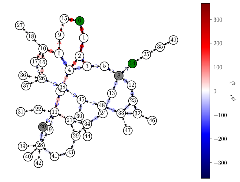
We deploy our proposed traffic-shaping scheme on the Anaheim city dataset [24]. For demonstration purposes, we only consider a sub-network of Anaheim consisting of 50 nodes and 118 edges presented in Figure 2, which includes some additional edges to ensure path connectivity of the sub-network.

The parameters $a_{\varepsilon},b_{\varepsilon},h_{\varepsilon}$ are derived from Anaheim’s original non-linear data via linearization as in [15]. We let $\eta_{i}=30\,[\$/\text{hr}]$ for all agents, while $q_{i}$ is drawn uniformly at random in the interval $[20,60]$. We assume the presence of two charging stations located at nodes $0$ and $14$, hence $\mathcal{C}^{\textup{c}}=\{0,14\}$. The associated prices are set to $\overline{c}_{0}^{\textup{c}}=0.35\,[\$/\text{kWh}]$ and $\overline{c}_{14}^{\textup{c}}=0.3\,[\$/\text{kWh}]$. Similarly, parking are located in nodes $8$ and $20$, hence $\mathcal{C}^{\textup{p}}=\{8,20\}$, and the prices are $\overline{c}_{8}^{\textup{p}}=17\,\$$ and $\overline{c}_{20}^{\textup{p}}=20\,\$$. The provided discounts are restricted to $c_{i}^{\textup{c},j}\in[0,0.2]$, for all $i\in\mathcal{N},j\in\mathcal{C}^{\textup{c}}$, whereas $c_{i}^{\textup{p},j}\in[0,5]$, for all $i\in\mathcal{N},j\in\mathcal{C}^{\textup{p}}$. The access rate of class $i$ to facility $j$ is set to $\delta_{i}^{c,j}=0.75\frac{P_{i}}{n_{\textup{c}}}$ and $\delta_{i}^{p,j}=0.75\frac{P_{i}}{n_{\textup{p}}}$ for all $i\in\mathcal{N},j\in\mathcal{C}$.

We consider $20$ classes of PEV s and $20$ classes of FV s that amount to $5\%$ and $15\%$ of the total vehicles for their respective type, ensuring a policy penetration rate of $20\%$. Given the total vehicles $n_{\text{veh}}=242584$ on the network, each class size is computed as $P_{i}=\rho_{i}\frac{n_{\text{veh}}}{20}$, where $\rho_{i}=0.05$ if $i$ is composed of PEVs and $\rho_{i}=0.20$ otherwise. For each PEVs class, the minimum fraction of vehicles that need to charge, i.e., $\bar{g}_{i}^{c}$, is randomly selected.

We investigate the TTT reduction attained by our algorithm as a function of the available budget. We consider both personalized and uniform discounts, where the latter correspond to providing the same discount to all agents that access a particular facility, i.e., $\mathcal{D}$ is endowed for every $j\in\mathcal{C}$ with the additional constraints $c_{i}^{\textup{c},j}=c_{\ell}^{\textup{c},j}$ and $c_{i}^{\textup{p},j}=c_{\ell}^{\textup{p},j}$ for all $i,\ell\in\mathcal{N}$. In Figure 3, we present the TTT reduction as a percentage of the TTT without intervention.

We observe that for large budgets both personalized and uniform incentives perform similarly, and are able to provide sensible decongestion of the network, around $3\%$. The magnitude of the result is inline with those obtain in other works considering incentives. For example, in an experiment performed in Lee county almost $17\text{M}\,\$$ has been put in place to achieve a traffic reduction of around $5\%$ see [25].

In our case, as the available budget decreases, personalized incentives outperform uniform ones due the more efficient and targeted allocation of resources. As an example to showcase the effect of the TA’s discounting policy on the routing game, we report in Figure 4 the difference in the flow of controllable vehicles, i.e., PEV and FV, with and without TA intervention, considering a budget of 5000 $. In this specific setting, the TA tends to offer discounts in the facility placed at node 0 to convey more vehicles towards that node and decongesting areas around remaining facilities, resulting in a decrement of the TTT of $76\,\text{h}$ every day.

Next, we explore the scalability of our proposed scheme by considering sub-networks of Anaheim of increasing size, starting form $n_{{v}}=50$ to $n_{{v}}=400$. We consider the computational cost of the TA’s updates, in the outer loop, and the agents’ updates, in the inner loop. Specifically, assuming a distributed implementation, the inner loop cost corresponds to the maximum computation time among all the agents. In Figure 5, we present both computational costs as a function of the number of nodes in the network.

To asses the overall computation time, we highlight that the number of outer loop iterations required for convergence is typically in the order of hundreds. Moreover, we can employ large tolerances for the inner loop iteration as in [16, Section V], which allow running few inner iterations (usually only one) for each outer loop iteration.

References

- [1] A. Schroten, H. van Essen, L. van Wijngaarden, D. Sutter, and E. Andrew, “Sustainable transport infrastructure charging and internalisation of transport externalities: Executive summary,” European Commission, Tech. Rep., May 2019.
- [2] M. Barth and K. Boriboonsomsin, “Traffic congestion and greenhouse gases,” Access Magazine, vol. 1, no. 35, pp. 2–9, 2009.
- [3] M. Beckmann, C. B. McGuire, and C. B. Winsten, “Studies in the economics of transportation,” Tech. Rep., 1956.
- [4] A. De Palma, M. Kilani, and R. Lindsey, “Congestion pricing on a road network: A study using the dynamic equilibrium simulator metropolis,” Transportation Research Part A: Policy and Practice, vol. 39, no. 7-9, pp. 588–611, 2005.
- [5] A. De Palma and R. Lindsey, “Traffic congestion pricing methodologies and technologies,” Transportation Research Part C: Emerging Technologies, vol. 19, no. 6, pp. 1377–1399, 2011.
- [6] M. Alizadeh, H.-T. Wai, M. Chowdhury, A. Goldsmith, A. Scaglione, and T. Javidi, “Optimal pricing to manage electric vehicles in coupled power and transportation networks,” IEEE Transactions on Control of Network Systems, vol. 4, no. 4, pp. 863–875, 2017.
- [7] S. R. Etesami, W. Saad, N. B. Mandayam, and H. V. Poor, “Smart routing of electric vehicles for load balancing in smart grids,” Automatica, vol. 120, p. 109148, 2020.
- [8] D. Paccagnan, R. Chandan, B. L. Ferguson, and J. R. Marden, “Optimal taxes in atomic congestion games,” ACM Transactions on Economics and Computation (TEAC), vol. 9, no. 3, pp. 1–33, 2021.
- [9] E. T. Verhoef, “Second-best congestion pricing in general networks. heuristic algorithms for finding second-best optimal toll levels and toll points,” Transportation Research Part B: Methodological, vol. 36, no. 8, pp. 707–729, 2002.
- [10] S. Lawphongpanich and D. W. Hearn, “An mpec approach to second-best toll pricing,” Mathematical programming, vol. 101, no. 1, pp. 33–55, 2004.
- [11] Y. Wang and D. Paccagnan, “Data-driven robust congestion pricing,” in 2022 IEEE 61st Conference on Decision and Control (CDC), 2022, pp. 4437–4443.
- [12] B. Sohet, Y. Hayel, O. Beaude, and A. Jeandin, “Hierarchical coupled driving-and-charging model of electric vehicles, stations and grid operators,” IEEE Transactions on Smart Grid, vol. 12, no. 6, pp. 5146–5157, 2021.
- [13] ——, “Coupled charging-and-driving incentives design for electric vehicles in urban networks,” IEEE Transactions on Intelligent Transportation Systems, vol. 22, no. 10, pp. 6342–6352, 2020.
- [14] B. G. Bakhshayesh and H. Kebriaei, “Decentralized equilibrium seeking of joint routing and destination planning of electric vehicles: A constrained aggregative game approach,” IEEE Transactions on Intelligent Transportation Systems, vol. 23, no. 8, pp. 13 265–13 274, 2022.
- [15] D. Calderone, E. Mazumdar, L. J. Ratliff, and S. S. Sastry, “Understanding the impact of parking on urban mobility via routing games on queue-flow networks,” in 2016 IEEE 55th Conference on Decision and Control (CDC), 2016, pp. 7605–7610.
- [16] P. D. Grontas, G. Belgioioso, C. Cenedese, M. Fochesato, J. Lygeros, and F. Dörfler, “BIG Hype: Best Intervention in Games via Distributed Hypergradient Descent,” 2023. [Online]. Available: https://arxiv.org/abs/2303.01101
- [17] L. Ambühl, A. Loder, M. Menendez, and K. W. Axhausen, “A case study of zurich’s two-layered perimeter control,” in 7th Transport Research Arena (TRA 2018). IVT, ETH Zurich, 2018.
- [18] F. Facchinei and J.-S. Pang, Finite-dimensional variational inequalities and complementarity problems. Springer, 2003.
- [19] M. Fochesato, C. Cenedese, and J. Lygeros, “A stackelberg game for incentive-based demand response in energy markets,” in 2022 IEEE 61st Conference on Decision and Control (CDC), 2022, pp. 2487–2492.
- [20] F. Fabiani, M. A. Tajeddini, H. Kebriaei, and S. Grammatico, “Local Stackelberg equilibrium seeking in generalized aggregative games,” IEEE Transactions on Automatic Control, vol. 67, no. 2, pp. 965–970, 2022.
- [21] J. Bolte and E. Pauwels, “Conservative set valued fields, automatic differentiation, stochastic gradient method and deep learning,” Mathematical Programming, Apr. 2020. [Online]. Available: https://hal.archives-ouvertes.fr/hal-02521848
- [22] B. Stellato, G. Banjac, P. Goulart, A. Bemporad, and S. Boyd, “OSQP: an operator splitting solver for quadratic programs,” Mathematical Programming Computation, vol. 12, no. 4, pp. 637–672, 2020. [Online]. Available: https://doi.org/10.1007/s12532-020-00179-2
- [23] B. Amos and J. Z. Kolter, “Optnet: Differentiable optimization as a layer in neural networks,” arXiv preprint arXiv:1703.00443, 2017.
- [24] Transportation Networks for Research Core Team, “Transportation networks for research,” accessed January 14, 2023. [Online]. Available: https://github.com/bstabler/TransportationNetworks
- [25] M. Burris and C. Swenson, “Planning Lee County’s Variable-Pricing Program,” Transportation Research Record, vol. 1617, no. 1, pp. 64–68, 1998. [Online]. Available: https://doi.org/10.3141/1617-09
Appendix
A Proof of Lemma 1
A sufficient condition for existence and uniqueness of a NE is that the PG is strongly monotone [18, Th. 2.3.3(b)]. Since is an affine mapping, strong monotonicity is equivalent to being positive definite [18, Th. 2.3.2(c)].
Observe that the functions and depend only on and , respectively. Therefore, after applying an appropriate permutation we can express as , where and . In the proof of [14, Lem. 1] it is shown , provided that is an affine function. Moreover, because is a strongly convex quadratic that depends only on , for all . The fact the both and are positive definite implies that , hence completing the proof.
B Proof of Proposition 1
To prove the claim, we will verify that Assumption 1 and Standing Assumptions 14 in [16] are satisfied by our model and then invoke [16, Th. 2]. Notice that the ’s are convex quadratic in the form of [16, Eq. 17], hence Assumption 1 holds. Further, Standing Assumption 1 holds true since the feasible sets are polyhedral. For Standing Assumption 2, we showed in the proof of Lemma 1 that is strongly monotone for any . Uniform strong monotonicity and Lipschitz continuity follows from the fact the is affine in . Standing Assumption 3 holds since is affine which implies that it is semialgebraic and, thus, definable. Finally, note that is semialgebraic, which implies definable, and is convex and compact, hence, verifying Standing Assumption 4.