Local Energy Distribution Based Hyperparameter Determination for Stochastic Simulated Annealing
Abstract
This paper presents a local energy distribution based hyperparameter determination for stochastic simulated annealing (SSA). SSA is capable of solving combinatorial optimization problems faster than typical simulated annealing (SA), but requires a time-consuming hyperparameter search. The proposed method determines hyperparameters based on the local energy distributions of spins (probabilistic bits). The spin is a basic computing element of SSA and is graphically connected to other spins with its weights. The distribution of the local energy can be estimated based on the central limit theorem (CLT). The CLT-based normal distribution is used to determine the hyperparameters, which reduces the time complexity for hyperparameter search from of the conventional method to . The performance of SSA with the determined hyperparameters is evaluated on the Gset and K2000 benchmarks for maximum-cut problems. The results show that the proposed method achieves mean cut values of approximately 98% of the best-known cut values.
Keywords Combinatorial optimization Hamiltonian Ising model simulated annealing stochastic computing.
1 INTRODUCTION
Combinatorial optimization is used to solve many practical problems in various fields and involves finding the optimal solution for a given objective function subject to a set of constraints Yarkoni et al. 2022. Combinatorial optimization problems are often NP-hard, meaning that finding the optimal solution requires an exponentially large amount of time with respect to the problem size Reiter and Johnson 2012. One such approach is simulated annealing, which is a stochastic optimization method inspired by the physical annealing process in materials science Kirkpatrick et al. 1983; Johnson et al. 1981. SA has been successfully applied to various combinatorial optimization problems, such as the traveling salesman problem, the graph coloring problem, and the maximum cut problem Mykleburst 2015. Quantum annealing (QA) is another optimization method that uses quantum mechanics to solve combinatorial optimization problems Kadowaki and Nishimori 1998; Boixo et al. 2014. It employs quantum devices that exploit quantum superposition and entanglement to explore the search space more efficiently than classical algorithms Neven 2016; however, QA devices are still in the early stage of development and have limited qubit coherence times and connectivity, which restricts their ability to solve large-scale problems Whittaker 2018.
Recently, a novel method known as stochastic-computing-based simulated annealing (SSA) has been introduced, which significantly expedites the annealing process compared to traditional SA and QA methods Onizawa et al. 2022 (to appear. SSA is a parallel variant of simulated annealing that utilizes an approximation of probabilistic bits (p-bits) Camsari et al. 2017, implemented through stochastic computing Gaines 1969; Brown and Card 2001. Its flexibility allows for implementation in both software and hardware Shin et al. 2023, potentially scaling up to handle large-scale problems. Combinatorial optimization problems are expressed using an Ising model Lucas 2014, which comprises spin states denoted as , spin biases symbolized by , and weights between spins represented by . The Ising model embodies an energy. In SSA, a pseudo inverse temperature is incrementally raised to determine a solution that corresponds to the global minimum energy, using random signals. To enhance performance (i.e., to increase the likelihood of reaching the global minimum energy), hyperparameters related to the pseudo inverse temperature and the random signals must be fine-tuned. This process, however, can be time-consuming due to the significant computational cost involved.
In this paper, we introduce a statistical method for determining hyperparameters for SSA that can eliminate the time-consuming hyperparameter search. In the proposed method, the hyperparameters are calculated based on the local energy distributions of spins. The local energy at each spin is calculated by the spin bias and the summation of the multiplication of the spin weights and other spin states. As the number of connections from the other spins is sufficiently large, the distribution of the local energy can be estimated based on the central limit theorem (CLT). Therefore, the local-energy distribution can be approximated by the normal distribution, which determines the hyperparameters, such as the pseudo inverse temperature and the noise signals. Compared with a conventional method that uses a grid search (i.e. typical hyperparameter search) in Onizawa et al. 2022 (to appear, the time complexity for the hyperparameter search is reduced to from . Using the determined hyperparameters, a unique noise control at each spin is also introduced for SSA to enhance the performance. The determined hyperparameters are evaluated in maximum-cut (MAX-CUT) problems Burer et al. 2001 that are a typical combinatorial optimization problem. On the MAX-CUT problem benchmarks, such as Gset Ye 1999 and K2000 Inagaki et al. 2016, the mean cut values using the proposed method reach approximately 98% of the best-known cut values for 1,000 cycles.
The contributions of the paper are:
- 1.
Introducing a new statistical method for determining hyperparameters in SSA that can eliminate the time-consuming hyperparameter search required by the conventional method.
- 2.
Demonstrating the effectiveness of the proposed method in solving the MAX-CUT problems and achieving mean cut values that are close to the best-known cut values.
- 3.
Reducing the time complexity for hyperparameter search from to compared to the conventional method.
The rest of the paper is structured as follows. section 2 reviews SSA and its hyperparameters. section 3 presents the proposed statistical method for determining the hyperparameters in SSA. section 4 introduces the unique noise magnitude for each spin. section 5 evaluates the determined hyperparameters and compares SSA with conventional SA. section 6 discusses the hyperparameter determination with the conventional hyperparameter search. Finally, section 7 concludes the paper.
2 PRELIMINARY
2.1 Stochastic simulated annealing (SSA)
There are several SA methods, such as serial updating Mykleburst 2015 and parallel tempering Gyoten et al. 2018. Recently, SSA has been presented as one of the SA methods Onizawa et al. 2022 (to appear. SSA is designed based on p-bit-based SA (pSA), which was introduced in Camsari et al. 2019. A p-bit is a probabilistic bit that can be one of two spin states, ‘+1’ and ‘-1’. It has been proposed for use in invertible logic, an unconventional computing technique Camsari et al. 2017; Smithson et al. 2019; Onizawa et al. 2020. pSA, implemented on an underlying Boltzmann machine Hinton et al. 1984, realizes parallel updating of the spins for fast simulated annealing. SSA approximates the behavior of p-bit using stochastic computing, which overcomes the slow convergence to the global minimum energy of pSA. Compared to other SA methods, SSA achieved the highest maximum-cut value in K2000 Katsuki et al. 2022.

fig. 1 illustrates SSA, which is on a spin network designed using spins, spin biases , and spin weights between spins. Each spin state can be either ‘-1’ and ‘+1’. The spin network is an Ising model Lucas 2014 that represents a Hamiltonian (energy function) as follows:
| (1) |
To solve a combinatorial optimization problem, the problem is mapped to the Hamiltonian coefficients of and . The coefficients differ depending on the problem, such as graph isomorphism and MAX-CUT problems Zick et al. 2015; Burer et al. 2001. During the annealing process, spin states are flipped between ‘+1’ and ‘-1’ in an attempt to reach the global minimum of the Hamiltonian.
In SSA, the spin behavior is modeled by approximating the p-bit using integral stochastic computing (ISC) Ardakani et al. 2017. Note that ISC is an extended version of typical stochastic computing Gaines 1969; Brown and Card 2001, which can be used for area-efficient hardware implementation Gaudet and Rapley 2003; Li et al. 2014; Liu and Parhi 2016. An -th spin has a bias and edge weights from/to other spins. At each cycle, the spin state is updated as follows:
| (2a) | |||
| (2b) | |||
| (2c) |
where and is binary input and output spin states, respectively. and are real-valued internal signals and is the magnitude of a random signal, . is the pseudo inverse temperature and is the minimum resolution of data representation. If only integer values are used in eq. 2c, is 1 Onizawa et al. 2022 (to appear. If floating-point values are used, can be approximated by 0.
2.2 Hyperparameter search for SSA
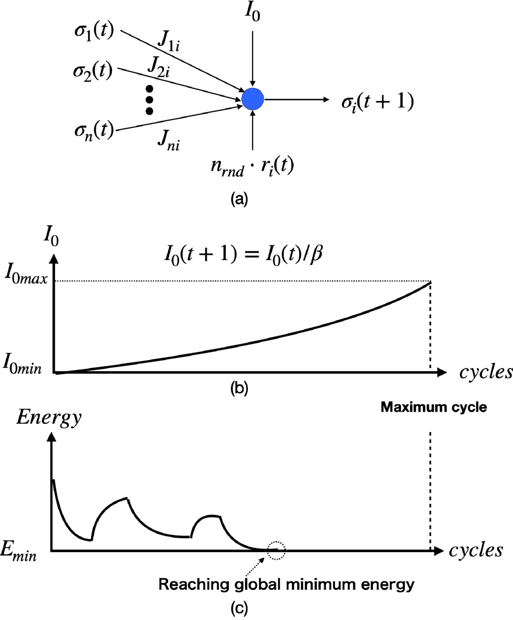
Let us explain the annealing process of SSA using fig. 2. At each cycle, is gradually increased from to as . The parameter controls the strength of the external field that acts on each spin. When is small, the spin states can be easily flipped to search for many spin states. This helps the spin states escape from local energy minima and explore a wider region of the solution space. When is large, the spin states can be stabilized in an attempt to reach the global minimum energy. Additionally, is an important parameter used to control the stability of the spin states.

To achieve a high probability of reaching the global minimum energy, the three hyperparameters of , and need to be carefully selected. In previous studies Onizawa et al. 2022 (to appear; Katsuki et al. 2022, a grid search or a random search has been used to select these hyperparameters, as shown in fig. 3 (a). In a grid search, a search space is defined as a grid of hyperparameter values, and every position in the grid is evaluated. In a random search, a search space is defined as a bounded domain of hyperparameter values, and points are randomly sampled within that domain. If good hyperparameters are not found, the search process is iteratively carried out until the required performance (e.g., probability of reaching the global minimum energy) is satisfied. While these methods are simple, they often require a long time to find good hyperparameters. In particular, when solving large combinatorial optimization problems, the time-consuming hyperparameter search could be a critical issue. In this paper, we determine the hyperparameters statistically by calculation, without performing a search, while achieving high performance of SSA, as shown in fig. 3 (b).
3 HYPERPARAMETER DETERMINATION BASED ON LOCAL ENERGY DISTRIBUTION
3.1 Local energy distribution

In the spin network, the spins interact with each other via pairwise interactions, which are often represented by the edge weights in a graph representation of the Ising model. The total energy of the spin network is defined as per eq. 1, whereas the local energy at the -th spin is defined as follows:
| (3) |
The local energy varies depending on the states of other spins that are connected to it with the edge weights . As the number of edges connected to a spin becomes larger, the distribution of the local energy becomes more and more Gaussian, which can be explained by the central limit theorem (CLT). In this case, the random variables are the edge weights , and the sum is over all the edges connected to a spin.
In fig. 4 (a), the local energy distribution at the spin is illustrated, where is the total number of spins representing a combinatorial optimization problem. The -th spin connects edges to other spins with the edge weights . Note that is a vector containing all the edge weights connected to the -th spin. Using CLT, the local energy distribution can be approximated by a normal distribution with mean and standard deviation calculated as follows:
| (4a) | |||
| (4b) |
where the semicolon is used to indicte concatenation of the two vectors.
3.2 Hyperparameter determination
fig. 4 (b) illustrates how to determine the three hyperparameters of , , and using the local energy distribution. As the three hyperparameters are common for all the spins, as shown in eq. 2c, the mean of the local energy distributions are considered. In other words, a normal distribution is used to control that commonly controls for all the spins.
First, the magnitude of noise signals is determined as follows:
| (5) |
The reason to select 0.6745 is that the point where the area from the mean of the normal distribution equals 50% is at 0.6745 from the mean. It means that the local energy distribution can be equally divided into two area by . Second, the minimum pseudo inverse temperature is determined as follows:
| (6) |
is set as close to as possible to facilitate the flipping of the spin states. Third, the maximum pseudo inverse temperature is determined as follows:
| (7) |
It means that a cumulative probability within a distance of from the mean is approximately 95%. The reasoning behind the selection of max/min functions originates from the local energy distribution. Each local distribution at its spin has different and , varying from small to large values. The usage of the max and min functions ensures that can encompass all local energy distributions by changing to during the annealing process.
4 SSA WITH UNIQUE NOISE MAGNITUDE (SSAU)

In SSA, the magnitude of the noise signals is common for all spins, as shown in fig. 5 (a). However, each spin has a unique local energy distribution that is different from others. To properly control the noise magnitude for each spin, SSA with a unique noise magnitude (SSAU) is introduced as an extension of SSA. This approach aims to better control the noise level for each spin and improve the search performance.
fig. 5 (b) shows SSAU with a unique noise magnitude for the -th spin. The noise magnitude for SSA in eq. 5 is updated for SSAU as follows:
| (8) |
where is the standard deviation of the local energy distribution at -th spin in eq. 4b. The other hyperparameters for SSAU are the same as that of SSA as shown in table 1.
5 EVALUATION
5.1 Simulation setup

The proposed statistical methods for determining hyperparameters are evaluated on maximum-cut (MAX-CUT) problems, which are a typical class of combinatorial optimization problems Burer et al. 2001. An example of a five-node MAX-CUT problem with edge weights of and is shown in fig. 6. The objective of MAX-CUT is to maximize the sum of edge weights by dividing the graph into two groups through a line cut. The annealing process changes the spin states in an attempt to reach the global minimum energy described in eq. 1, where the maximum cut value is corresponding to the global minimum energy. The black circle illustrates a spin state of ’+1’, while the white circle illustrates a spin state of ’-1’. In this example, the graph is divided into Group A (nodes 2, 3, and 4) and Group B (nodes 1 and 5), with a sum of edge weights equal to 4. The edge weights are represented using in the Hamiltonian shown in eq. 1.
| Graph | # nodes | Structure | Weights () | # edges |
|---|---|---|---|---|
| G1 | 800 | random | 19176 | |
| G6 | 800 | random | 19176 | |
| G11 | 800 | toroidal | 1600 | |
| G14 | 800 | planar | 4694 | |
| G18 | 800 | planar | 4694 | |
| G22 | 2000 | random | 19990 | |
| G34 | 2000 | toroidal | 4000 | |
| G38 | 2000 | planar | 11779 | |
| G39 | 2000 | planar | 11778 | |
| G47 | 1000 | random | 9990 | |
| G48 | 3000 | toroidal | 6000 | |
| G54 | 1000 | random | 5916 | |
| G55 | 5000 | random | 12498 | |
| G56 | 5000 | random | 12498 | |
| G58 | 5000 | planar | 29570 | |
| K2000 | 2000 | full | 1999000 |
table 2 summarizes the benchmarks for the MAX-CUT problems that are used to evaluate the proposed method. The Gset includes the Gx graphs with different sizes, shapes, and weights Ye 1999, while K2000 is another benchmark that consists of fully-connected graphs with 2,000 nodes Inagaki et al. 2016. All simulation results are obtained using Python 3.9.6 on an Apple M1 Ultra with 128 GB of memory.
5.2 Determined hyperparameters
| Graph | SSA | SSAU | ||||
|---|---|---|---|---|---|---|
| G1 | [26.97, 66.92] | [5.19, 8.18] | 4.66 | 27.05 | 43.33 | [3.50, 5.52] |
| G6 | [0.00, 28.96] | [5.19, 8.18] | 4.66 | 0.08 | 16.36 | [3.50, 5.52] |
| G11 | [0.00, 3.99] | [1.99, 1.99] | 1.35 | 0.02 | 3.99 | [1.35, 1.35] |
| G14 | [4.99, 131.84] | [2.23, 11.48] | 2.18 | 5.11 | 27.96 | [1.50, 7.74] |
| G18 | [0.00, 17.98] | [2.23, 11.48] | 2.18 | 0.11 | 22.96 | [1.50, 7.74] |
| G22 | [6.99, 36.98] | [2.64, 6.08] | 2.99 | 7.05 | 19.16 | [1.78, 4.10] |
| G34 | [0.00, 3.99] | [1.99, 1.99] | 1.35 | 0.02 | 3.99 | [1.35, 1.35] |
| G38 | [3.99, 248.88] | [1.99, 15.78] | 2.17 | 4.16 | 35.55 | [1.35, 10.64] |
| G39 | [0.00, 42.98] | [1.99, 14.49] | 2.17 | 0.14 | 28.97 | [1.35, 9.77] |
| G47 | [7.99, 33.97] | [2.83, 5.83] | 2.99 | 8.05 | 19.64 | [1.90, 3.93] |
| G48 | [3.99, 3.99] | [1.99, 1.99] | 1.35 | 4.02 | 7.99 | [1.35, 1.35] |
| G54 | [4.99, 135.86] | [2.23, 11.66] | 2.18 | 5.11 | 28.30 | [1.51, 7.86] |
| G55 | [0.00, 14.99] | [0.00, 3.87] | 1.46 | 0.03 | 7.75 | [0.00, 2.61] |
| G56 | [0.00, 9.99] | [0.00, 3.87] | 1.46 | 0.03 | 7.75 | [0.00, 2.61] |
| G58 | [3.99, 560.88] | [1.99, 23.68] | 2.17 | 4.24 | 51.36 | [1.35, 15.97] |
| K2000 | [0.99, 168.92] | [44.70, 44.70] | 30.15 | 1.45 | 90.40 | [30.15, 30.15] |

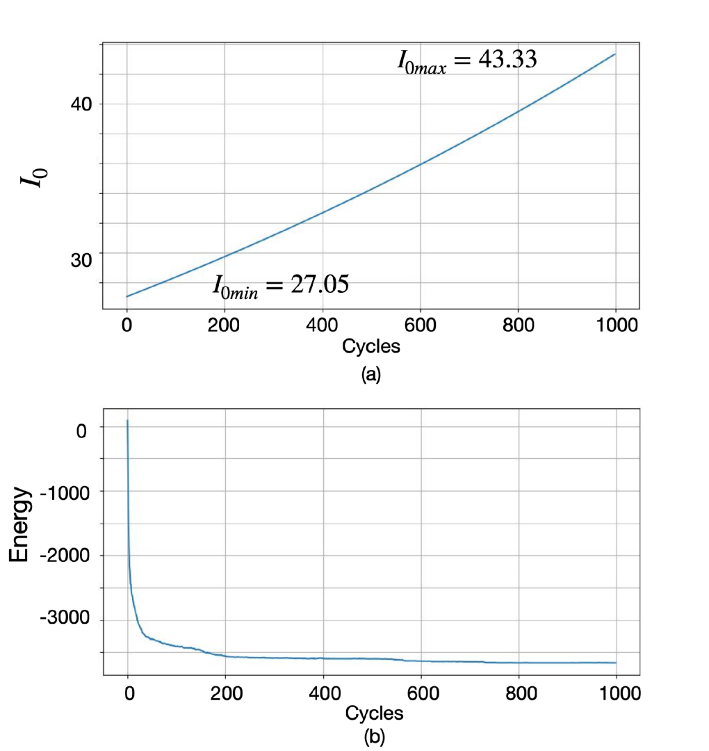
table 3 summarizes the hyperparameters used for SSA and SSAU. The equations for calculating these hyperparameters are provided in table 1 and eq. 8. To illustrate how these values are determined, let us consider the example of G1. The matrix of G1 is an 800800 matrix. It consists of edge weights either ‘+1’ or ‘0’, with the count of ‘+1’ edge weights being 19,176. The total number of edges in the matrix amounts to 319,600. First, and are calculated for each of the 800 vectors in , which yields a unique set of values for each spin. As an example, two normal distributions with the minimum and maximum values of are shown in fig. 7 (a). The range of is from 26.97 to 66.92, and the range of is from 5.19 to 8.18, as shown in fig. 7 (b).
Next, and are used to calculate the hyperparameters of , , and . In the case of SSAU, each spin has a unique value, which corresponds to its local energy distribution. The range of is from 3.50 to 5.52.
| Graph | Best known | Mean of cut values | Standard deviation of cut values | Ratio of mean cut value | ||||||
| cut value | SA Mykleburst 2015 | SSA | SSAU | SA | SSA | SSAU | SSA | SSAU | SSAU | |
| vs. SA | vs. SA | vs. SSA | ||||||||
| G1 | 800 | 10754.52 | 11427.05 | 11428.13 | 47.63 | 32.83 | 33.28 | 6.25% | 6.26% | 0.01% |
| G6 | 800 | 1276.96 | 2159.59 | 2160.63 | 45.56 | 12.29 | 12.44 | 69.12% | 69.20% | 0.05% |
| G11 | 800 | 334.98 | 549.60 | 549.47 | 13.16 | 4.12 | 4.10 | 64.07% | 64.03% | -0.02% |
| G14 | 800 | 2803.34 | 3009.71 | 3013.20 | 15.55 | 8.13 | 7.70 | 7.36% | 7.49% | 0.12% |
| G18 | 800 | 590.68 | 972.49 | 974.72 | 25.60 | 8.34 | 7.56 | 64.64% | 65.02% | 0.23% |
| G22 | 2000 | 11161.3 | 13099.78 | 13102.26 | 50.47 | 31.63 | 31.34 | 17.37% | 17.39% | 0.02% |
| G34 | 2000 | 469.26 | 1346.64 | 1346.67 | 27.97 | 6.34 | 6.39 | 186.97% | 186.98% | 0.00% |
| G38 | 2000 | 6642.68 | 7546.93 | 7554.4 | 31.09 | 15.82 | 15.71 | 13.61% | 13.73% | 0.10% |
| G39 | 2000 | 862.1 | 2352.47 | 2362.03 | 46.48 | 14.01 | 12.41 | 172.88% | 173.99% | 0.41% |
| G47 | 1000 | 5854.9 | 6536.24 | 6537.83 | 33.10 | 21.62 | 21.15 | 11.64% | 11.66% | 0.02% |
| G48 | 3000 | 3562.2 | 5724.25 | 5724.29 | 30.94 | 38.20 | 38.15 | 60.69% | 60.70% | 0.00% |
| G54 | 1000 | 3484.95 | 3780.36 | 3784.71 | 19.66 | 8.73 | 8.54 | 8.48% | 8.60% | 0.11% |
| G55 | 5000 | 6973.55 | 9994.42 | 10037.44 | 45.21 | 22.33 | 21.02 | 43.32% | 43.94% | 0.43% |
| G56 | 5000 | 702.21 | 3930.36 | 3947.27 | 55.74 | 14.72 | 12.08 | 459.71% | 462.12% | 0.43% |
| G58 | 5000 | 15791.8 | 18930.60 | 18949.24 | 68.81 | 27.41 | 30.40 | 19.88% | 19.99% | 0.10% |
| K2000 | 2000 | 11267.73 | 32931.54 | 32932.38 | 566.15 | 117.59 | 117.71 | 192.26% | 192.27% | 0.00% |
To verify the hyperparameters, SSA with G1 is simulated as an example. fig. 8 (a) illustrates the pseudo inverse-temperature transition for 1,000 cycles. is gradually increased from to . The value of is updated by , where . The energy, defined by eq. 1, decreases to the global minimum as increases. Once the simulation completes 1,000 cycles, the spin states are extracted to compute the cut value using .
5.3 Comparisons
table 4 compares SSA and SSAU with a conventional SA in the 16 different MAX-CUT problems for 1,000 cycles. Let us briefly explain the simulation conditions for SA, as detailed in Mykleburst 2015. In this method, the temperature is gradually decreased by as at each cycle. The initial temperature is set to 1, and the final temperature is set to 1/1000. The number of cycles is 1,000, which is the same as for SSA and SSAU. During each cycle, a spin state is randomly flipped, and a new state is accepted if the new energy () is lower than the current energy () or if it is higher with a probability of .
The mean and the standard deviation of cut values are obtained by running 100 trials for each benchmark. When comparing SSA and SSAU with SA, the ratios of the mean cut values are positive in all benchmarks. In particular, the ratios are significantly positive in the case of graphs with {+1, 0, -1} weights. The reason is that SA takes more cycles to achieve better cut values in the case, where the mean cut values are significantly smaller than the best-known values. The mean of normalized cut values is 65.0% for SA.
| SA | SSA | SSAU | |
|---|---|---|---|
| G1 | 10859 | 11550 | 11560 |
| G6 | 1389 | 2178 | 2178 |
| G11 | 364 | 564 | 564 |
| G14 | 2836 | 3040 | 3040 |
| G18 | 647 | 990 | 992 |
| G22 | 11325 | 13214 | 13221 |
| G34 | 536 | 1368 | 1368 |
| G38 | 6715 | 7603 | 7606 |
| G39 | 993 | 2399 | 2400 |
| G47 | 5947 | 6647 | 6615 |
| G48 | 3642 | 5934 | 5904 |
| G54 | 3530 | 3820 | 3815 |
| G55 | 7088 | 10073 | 10121 |
| G56 | 831 | 3982 | 3996 |
| G58 | 15919 | 19014 | 19033 |
| K2000 | 12413 | 33235 | 33225 |

| Conventional Onizawa et al. 2022 (to appear; Katsuki et al. 2022 | This work | |
|---|---|---|
| Time complexity |
| Conventional | This work | Normalized mean cut value | |||||
|---|---|---|---|---|---|---|---|
| Search time [s] | Annealing time [s] | Total time [s] | Annealing time | Conventional | This work | Ratio | |
| (total time) [s] | |||||||
| G1 | 310.61 | 0.28 | 310.88 | 0.40 | 98.58% | 98.31% | -0.28% |
| G6 | 286.76 | 0.26 | 287.02 | 0.28 | 89.51% | 99.15% | 10.78% |
| G11 | 313.34 | 0.28 | 313.62 | 0.40 | 88.1%4 | 97.45% | 10.56% |
| G14 | 312.60 | 0.25 | 312.85 | 0.39 | 97.44% | 98.23% | 0.81% |
| G18 | 316.05 | 0.28 | 316.32 | 0.29 | 87.90% | 98.03% | 11.53% |
| G22 | 1523.29 | 1.45 | 1524.74 | 1.45 | 97.4%2 | 98.06% | 0.66% |
| G34 | 1494.86 | 1.45 | 1496.30 | 1.80 | 94.66% | 97.30% | 2.79% |
| G38 | 1483.77 | 1.45 | 1485.21 | 1.83 | 96.95% | 98.17% | 1.26% |
| G39 | 1473.18 | 1.45 | 1474.63 | 1.83 | 87.2%3 | 97.69% | 12.00% |
| G47 | 433.96 | 0.41 | 434.37 | 0.61 | 96.92% | 98.18% | 1.31% |
| G48 | 3250.20 | 3.26 | 3253.46 | 4.19 | 88.33% | 95.40 % | 8.01% |
| G54 | 418.73 | 0.40 | 419.12 | 0.61 | 97.81% | 98.14% | 0.34% |
| G55 | 8812.68 | 8.96 | 8821.64 | 10.71 | 94.68% | 97.04% | 2.49% |
| G56 | 8869.97 | 8.80 | 8878.77 | 9.30 | 94.24% | 97.84% | 3.83% |
| G58 | 8794.97 | 8.82 | 8803.79 | 9.24 | 97.57% | 98.12% | 0.57% |
| K2000 | 1451.41 | 1.44 | 1452.85 | 1.52 | 98.24% | 98.78% | 0.56% |
When comparing SSA and SSAU, the mean cut values of SSAU are larger than that of SSA in most of the benchmarks. The ratios are relatively large in the case of graphs with {+1, 0} weights. The standard deviation of the cut values is similar for both methods, with these values significantly smaller than that of SA. On average, across all benchmarks for 1,000 cycles, the mean cut values of SSA and SSAU are 97.9% and 98.0% of the best-known cut values, respectively. In terms of computation cost, SSAU takes almost the same simulation time as SSA. For instance, the simulation time on K2000 for 1,000 cycles is 1.43 seconds for both SSA and SSAU. The best cut values are summarized in table 5. It shows that SSA and SSAU achieve 99.2% of the best-known cut values while SA only attains 67.7%.
fig. 9 displays the mean of normalized cut values in relation to the number of cycles for 16 benchmarks. Both SSA and SSAU quickly achieve an average of 95.4% of the normalized best-known value within just 100 cycles, while SA only reaches 48.2%. For 10,000 cycles, SA, SSA, and SSAU achieve 90.0%, 98.8%, and 98.9% respectively. Compared to related works on K2000, the mean cut value of SSAU is 32,932, which surpasses the 32,458 and 32,768 values from Inagaki et al. 2016 and Goto et al. 2019, respectively.
6 DISCUSSION
6.1 Comparison with hyperparameter search
The comparison result between SA and SSA for G11 was previously presented in Onizawa et al. 2022 (to appear. SSA achieved superior mean cut values compared to SA and QA, even though the previous study employed hyperparameter searching. table 6 provides a comparison of the time complexity of hyperparameter searching for SSA. In the conventional method Onizawa et al. 2022 (to appear; Katsuki et al. 2022, the hyperparameters of , , and were selected through searching, leading to a time complexity of . In contrast, the proposed method determines these hyperparameters statistically without the need for searching, thereby resulting in a time complexity of .
Let us discuss the impact of determined hyperparameters in SSA. As summarized in table 6, the conventional method necessitates the search for hyperparameters prior to simulated annealing. table 7 compares the search and annealing time, along with the normalized mean cut values for the all 16 benchmarks using SSA, where the annealing takes 1,000 cycles. In the conventional method, the hyperparameters of , , and are randomly searched for across 1,000 trials, with each value ranging from 0 to 1000 with a condition of . Based on these search results, the best hyperparameters are selected to evaluate the mean cut values. The outcome indicates that the proposed method, which excludes the hyperparameter search, yields results that are superior to the conventional method in most benchmarks. Moreover, the proposed method completely eliminates the time-consuming process of hyperparameter searching.

fig. 10 illustrates the normalized cut values using random search with 1,000 cycles on G58. In G58, the proposed method achieves a normalized mean cut value of 98.2%, which is superior to the 97.6% of the conventional method. Both the best hyperparameters identified through searching and the determined hyperparameters are plotted. The plotted values for and are similar between the conventional and proposed methods; however, the values for differ significantly, potentially leading to performance loss. As the search process iterates 1,000 times, more iterations might yield better hyperparameters, but this would also increase the search time.
6.2 Hyperparameter selection
Let us discuss the effect of using 0.01 for in eq. 6. In this study, the constant 0.01 is utilized to position close to . This results in a mean normalized cut value of 97.9% on average in SSA. When 0.01 is changed to or , the respective averages become 97.6% and 97.8%. Hence, the constant for does not significantly impact the results. Note that a value of 0 is not permissible. The range of this value is associated with the equation as shown in Table 1. If the value is 0, becomes 0 in several benchmarks, especially when is 0. This makes it impossible to determine . Therefore, is set to a value as low as .
Additionally, the number of standard deviations set to 2 for in eq. 7 is examined. To evaluate the impact of this standard deviation number, it is altered to 3 and 4. As a result, the mean normalized cut value averages 97.8% in SSA for both cases. Therefore, the constant for also does not have a significant effect on the results.

There might be a constraint of the proposed determined hyperparameters based on CLT when each spin contains a few connections. To assess the performance of the proposed method based on the number of connections, new benchmarks are created using K2000 as a reference. K2000 is fully connected with weights of +1 or -1, and the ratio of +1 to -1 weights is 50%. These benchmarks encompass spin counts ranging from 5 to 1000, with each spin being fully connected and assigned weights of either +1 or -1. The mean cut values, taken from 100 trials, are contrasted between the conventional search and the proposed method in fig. 11. The conventional method searches the best hyperparameters for 1,000 trials. The findings indicate that the proposed method outperforms the conventional approach when there is a larger number of connections. However, with a smaller number of connections, the assumptions underpinning the Central Limit Theorem (CLT) might not be met, even though the mean cut values remain nearly identical. A possible explanation is that annealing is effective with a smaller number of spins, even in the absence of precise hyperparameters.
7 CONCLUSION
This paper proposes the local energy distribution based hyperparameter determination in SSA, which is a faster solving method for combinatorial optimization problems than SA. The method is based on the local energy distributions of spins and utilizes the CLT-based normal distribution for hyperparameter determination, significantly reducing the time complexity for hyperparameter search. Additionally, using the local energy distributions, the unique magnitude for the random signal at each spin has been presented to further improve SSA. The proposed method is evaluated in the MAX-CUT problems, where it achieves high accuracy while reducing time costs compared to conventional SSA with hyperparameter search.
Future research directions include applying the proposed method to other optimization problems, exploring the impact of hyperparameters on the SSA performance, developing more efficient hardware.
Acknowledgment
This work was supported in part by JST CREST Grant Number JPMJCR19K3, and JSPS KAKENHI Grant Number JP21H03404.
References
- Yarkoni et al. [2022] Sheir Yarkoni, Elena Raponi, Thomas Bäck, and Sebastian Schmitt. Quantum annealing for industry applications: introduction and review. Reports on Progress in Physics, 85(10):104001, sep 2022. doi:10.1088/1361-6633/ac8c54. URL https://doi.org/10.1088%2F1361-6633%2Fac8c54.
- Reiter and Johnson [2012] Edna E. Reiter and Clayton Matthew Johnson. Limits of Computation: An Introduction to the Undecidable and the Intractable. Chapman and Hall/CRC, 2012. ISBN 1439882061.
- Kirkpatrick et al. [1983] Scott Kirkpatrick, Charles D Gelatt Jr, and Mario P Vecchi. Optimization by simulated annealing. Science, 220(4598):671–680, 1983.
- Johnson et al. [1981] David S Johnson, Cecilia R Aragon, Lyle A McGeoch, and Carla Schevon. Optimization by simulated annealing: An experimental evaluation; part ii, graph coloring and number partitioning. Operations Research, 39(3):378–406, 1981.
- Mykleburst [2015] Tor Mykleburst. Solving maximum cut problems by simulated annealing. CoRR, arXiv:1505.03068, 2015. URL https://arxiv.org/abs/1505.03068.
- Kadowaki and Nishimori [1998] Tadashi Kadowaki and Hidetoshi Nishimori. Quantum annealing in the transverse ising model. Physical Review E, 58(5):5355–5363, 1998.
- Boixo et al. [2014] Sergio Boixo, Troels F. Rønnow, Sergei V. Isakov, Zhihui Wang, David Wecker, Daniel A. Lidar, John M. Martinis, and Matthias Troyer. Evidence for quantum annealing with more than one hundred qubits. Nature Physics, 10(3):218–224, 2014. doi:10.1038/nphys2900. URL https://doi.org/10.1038/nphys2900.
- Neven [2016] Hartmut Neven. When can quantum annealing win?, Jan. 2016. URL https://ai.googleblog.com/2015/12/when-can-quantum-annealing-win.html.
- Whittaker [2018] J. Whittaker. System roadmap. D-Wave Systems, 2018.
- Onizawa et al. [2022 (to appear] Naoya Onizawa, Kota Katsuki, Duckgyu Shin, Warren J. Gross, and Takahiro Hanyu. Fast-converging simulated annealing for Ising models based on integral stochastic computing. IEEE Transactions on Neural Networks and Learning Systems, pages 1–7, 2022 (to appear). doi:10.1109/TNNLS.2022.3159713.
- Camsari et al. [2017] Kerem Camsari, Rafatul Faria, Brian Sutton, and Supriyo Datta. Stochastic p-bits for invertible logic. Physical Review X, 7, July 2017. doi:10.1103/PhysRevX.7.031014.
- Gaines [1969] B. R. Gaines. Stochastic computing systems. Adv. Inf. Syst. Sci. Plenum, 2(2):37–172, 1969. ISSN 0018-9340. doi:10.1109/12.954505.
- Brown and Card [2001] B. D. Brown and H. C. Card. Stochastic neural computation. I. computational elements. IEEE Transactions on Computers, 50(9):891–905, Sep. 2001. ISSN 0018-9340. doi:10.1109/12.954505.
- Shin et al. [2023] Duckgyu Shin, Naoya Onizawa, Warren J. Gross, and Takahiro Hanyu. Memory-efficient fpga implementation of stochastic simulated annealing. IEEE Journal on Emerging and Selected Topics in Circuits and Systems, 13(1):108–118, 2023. doi:10.1109/JETCAS.2023.3243260.
- Lucas [2014] Andrew Lucas. Ising formulations of many NP problems. Frontiers in Physics, 2:5, 2014. ISSN 2296-424X. doi:10.3389/fphy.2014.00005. URL https://www.frontiersin.org/article/10.3389/fphy.2014.00005.
- Burer et al. [2001] Samuel Burer, Renato D. C. Monteiro, and Yin Zhang. Rank-two relaxation heuristics for MAX-CUT and other binary quadratic programs. SIAM Journal on Optimization, 12(2):503–521, 2001.
- Ye [1999] Y. Ye. Computational optimization laboratory, 1999. URL http://web.stanford.edu/˜yyye/Col.htm.
- Inagaki et al. [2016] Takahiro Inagaki, Yoshitaka Haribara, Kensuke Igarashi, Tomohiro Sonobe, Shuhei Tamate, Toshimori Honjo, Alireza Marandi, Peter L McMahon, Takeshi Umeki, Kohei Enbutsu, and et al. A coherent ising machine for 2000-node optimization problems. Science, 354(6312):603–606, 2016.
- Gyoten et al. [2018] Hidenori Gyoten, Masayuki Hiromoto, and Takashi Sato. Enhancing the solution quality of hardware ising-model solver via parallel tempering. In Proceedings of the International Conference on Computer-Aided Design, ICCAD ’18, New York, NY, USA, 2018. Association for Computing Machinery. ISBN 9781450359504. doi:10.1145/3240765.3240806. URL https://doi.org/10.1145/3240765.3240806.
- Camsari et al. [2019] Kerem Yunus Camsari, Brian M. Sutton, and Supriyo Datta. p-bits for probabilistic spin logic. Applied Physics Reviews, 6:011305, 2019.
- Smithson et al. [2019] S. C. Smithson, N. Onizawa, B. H. Meyer, W. J. Gross, and T. Hanyu. Efficient CMOS invertible logic using stochastic computing. IEEE Transactions on Circuits and Systems I: Regular Papers, 66(6):2263–2274, June 2019. ISSN 1549-8328. doi:10.1109/TCSI.2018.2889732.
- Onizawa et al. [2020] N. Onizawa, S. C. Smithson, B. H. Meyer, W. J. Gross, and T. Hanyu. In-hardware training chip based on cmos invertible logic for machine learning. IEEE Transactions on Circuits and Systems I: Regular Papers, 67(5):1541–1550, May 2020. ISSN 1558-0806. doi:10.1109/TCSI.2019.2960383.
- Hinton et al. [1984] G. E. Hinton, T. J. Sejnowski, and D. H. Ackley. Boltzmann machines: Constraint satisfaction networks that learn. Technical Report CMU-CS-84-119, Department of Computer Science, Carnegie-Mellon University, 1984.
- Katsuki et al. [2022] Kota Katsuki, Duckgyu Shin, Naoya Onizawa, and Takahiro Hanyu. Fast solving complete 2000-node optimization using stochastic-computing simulated annealing. In 2022 29th IEEE International Conference on Electronics, Circuits and Systems (ICECS), pages 1–4, 2022. doi:10.1109/ICECS202256217.2022.9971124.
- Zick et al. [2015] Kenneth M. Zick, Omar Shehab, and Matthew French. Experimental quantum annealing: case study involving the graph isomorphism problem. Scientific Reports, 5(1):11168, 2015. doi:10.1038/srep11168. URL https://doi.org/10.1038/srep11168.
- Ardakani et al. [2017] A. Ardakani, F. Leduc-Primeau, N. Onizawa, T. Hanyu, and W. J. Gross. VLSI implementation of deep neural network using integral stochastic computing. IEEE Transactions on Very Large Scale Integration (VLSI) Systems, 25(10):2588–2599, Oct. 2017. ISSN 1063-8210. doi:10.1109/TVLSI.2017.2654298.
- Gaudet and Rapley [2003] V. C. Gaudet and A. C. Rapley. Iterative decoding using stochastic computation. Electronics Letters, 39(3):299 – 301, Feb. 2003. ISSN 0013-5194. doi:10.1049/el:20030217.
- Li et al. [2014] P. Li, D. J. Lilja, W. Qian, K. Bazargan, and M. D. Riedel. Computation on stochastic bit streams digital image processing case studies. IEEE Transactions on Very Large Scale Integration (VLSI) Systems, 22(3):449–462, Mar. 2014. ISSN 1063-8210. doi:10.1109/.2013.2247429.
- Liu and Parhi [2016] Y. Liu and K. K. Parhi. Architectures for recursive digital filters using stochastic computing. IEEE Transactions on Signal Processing, 64(14):3705–3718, July 2016. ISSN 1053-587X. doi:10.1109/TSP.2016.2552513.
- Goto et al. [2019] Hayato Goto, Kosuke Tatsumura, and Alexander R. Dixon. Combinatorial optimization by simulating adiabatic bifurcations in nonlinear hamiltonian systems. Science Advances, 5(4):eaav2372, 2019. doi:10.1126/sciadv.aav2372. URL https://www.science.org/doi/abs/10.1126/sciadv.aav2372.