The Disharmony between BN and ReLU Causes Gradient Explosion, but is Offset by the Correlation between Activations

Inyoung Paik Jaesik Choi Affiliation: KAIST, South Korea Affiliation: {humandream, jaesik.choi}@kaist.ac.kr

Abstract

Deep neural networks, which employ batch normalization and ReLU-like activation functions, suffer from instability in the early stages of training due to the high gradient induced by temporal gradient explosion. In this study, we analyze the occurrence and mitigation of gradient explosion both theoretically and empirically, and discover that the correlation between activations plays a key role in preventing the gradient explosion from persisting throughout the training. Finally, based on our observations, we propose an improved adaptive learning rate algorithm to effectively control the training instability.

1 Introduction

The success of deep neural networks stems from their remarkable expressive power, which grows exponentially with increasing depth (Chatziafratis et al. 2019). However, the deep hierarchical architecture of these networks can give rise to the problem of exploding/vanishing gradients (Goodfellow et al. 2016), which significantly impairs performance and may render training infeasible.

Some studies (Philipp et al. 2017; Yang et al. 2019) have shown that gradient explosion can occur in modern neural networks, showing that a stable flow of the forwarding signal does not guarantee a stable flow of backward gradient. However, since the advent of normalization methods (Ioffe & Szegedy 2015; Ulyanov et al. 2016; Ba et al. 2016; Wu & He 2018; Qiao et al. 2019), it appears that gradient explosion is no longer a serious issue and is often regarded as a problem of the past.

However, we note that gradient explosion actually exists in the variety of modern deep neural networks with ReLU and batch normalization (Ioffe & Szegedy 2015) in the initialization state. However, due to the rapid changes in training dynamics, different terminologies have been used to describe this problem, like ‘large gradient magnitude at the early stage of training’ or ‘instability of deep neural networks in the early phase of training’ (Frankle et al. 2020; Goyal et al. 2017b). It is also often addressed as an ‘instability problem of large batch training’ (Goyal et al. 2017b), as the severity of the issue escalates when using a large batch size (alongside a correspondingly high learning rate) during training.

The disparity between theory and practice has hindered the resolution of this problem, and practical solutions have been developed relying on empirical experience and intuition. In this paper, we aim to offer a more precise diagnosis of the problem and propose a more efficient solution derived from this diagnosis.

Refer to caption — Figure 1: Gradient explosion rate ( $\sqrt{\mathrm{Var}(g^{n})/\mathrm{Var}(g^{N})}$ ) of deep neural network models at the initialization state corresponding to different architectures (left) and activation functions (right). The explosion rate is approximately $\sqrt{\pi/(\pi-1)}$ in vanilla networks with batch normalization. However, it is lower in architectures with residual connections (He et al. 2016), which reduces the effective depth. (Philipp et al. 2017) No evidence of gradient explosion was observed in architectures without batch normalization, including transformer-based architectures (Dosovitskiy et al. 2020).
The figure on the right is plotted using VGG (Simonyan & Zisserman 2014) architecture with different activation functions. Smoother variants of ReLU (Maas et al. 2013; Clevert et al. 2015; Ramachandran et al. 2017; Hendrycks & Gimpel 2016) exhibit lower explosion rates due to their flatter behavior near the origin. It is worth noting that gradient explosion does not occur with DropOut (Srivastava et al. 2014), which can be regarded as a ReLU that randomly blocks signals.

2 How Gradient Explosion Occurs

As weights are repeatedly multiplied during forward/backward propagation, the exploding or vanishing gradient problem is commonly believed to be caused by excessively large or small parameters (Bengio et al. 1994; Pascanu et al. 2013). Consequently, it has often been regarded as a problem related to the initialization and maintenance of appropriate weight scales. (He et al. 2015) assumed that initializing weight with $N(0,\sqrt{2/n_{out}})$ would maintain similar variances in both forward and backward propagation. In this perspective, this problem was seen as potentially ‘solved’ with the introduction of (batch) normalization (Ioffe & Szegedy 2015), which automatically corrects suboptimal choices of weight scales.

However, it is important to consider how the activation function affects the input distribution. Figure 2 illustrates that using the positive part of the activation differs from randomly blocking selected activations. In short, (He et al. 2015) described the scenario assuming DropOut (Srivastava et al. 2014) as the activation function rather than ReLU. In this case, both the forward and backward signals are roughly halved, preventing the occurrence of either exploding or vanishing gradients. However, real activation functions are highly dependent on the forward signal while being almost uncorrelated with the backward gradient. This discrepancy can lead to differential effects on the variance during forward and backward propagation (Philipp et al. 2017).

Proposition 2.1.

Let $X=\mathrm{ReLU}(Y)=max(Y,0)$ , where $Y\sim N(\mu,\sigma^{2})$ . Then, we have:

\displaystyle\mathbb{E}(X)=\mu(1-\phi(-\frac{\mu}{\sigma}))+\frac{\sigma}{\sqrt{2\pi}}e^{-\frac{\mu^{2}}{2\sigma^{2}}}

(1)

\displaystyle\mathrm{Var}(X)

\displaystyle=(\sigma^{2}+\mu^{2})(1-\phi(-\frac{\mu}{\sigma}))+\mu\frac{\sigma}{\sqrt{2\pi}}e^{-\frac{\mu^{2}}{2\sigma^{2}}}-(\mu(1-\phi(-\frac{\mu}{\sigma}))+\frac{\sigma}{\sqrt{2\pi}}e^{-\frac{\mu^{2}}{2\sigma^{2}}})^{2}

(2)

where $\phi(x)=\int_{-\infty}^{x}\frac{1}{\sqrt{2\pi}}e^{-x^{2}/2}$ is the cumulative distribution function of the standard normal distribution.

Proof.

See Appendix A.1 ∎

Theorem 2.2.

Consider the repetitive neural network architecture $f^{n}:\mathbb{R}^{d_{n}}\longmapsto\mathbb{R}^{d_{n+1}}$ . Let $x^{n+1}=f^{n}(x^{n})=\mathrm{BatchNorm}(W^{n}(\mathrm{ReLU}(x^{n}))+b^{n})=\frac{W^{n}(\mathrm{ReLU}(x^{n}))+b^{n}-\hat{\mu}}{\hat{\sigma}}\gamma^{n+1}+\beta^{n+1}$ , where $\gamma^{n+1},\beta^{n+1}\in\mathbb{R}^{d_{n+1}}$ are affine transformation parameters, and $\hat{\mu},\hat{\sigma}\in\mathbb{R}^{d_{n+1}}$ are the estimated mean and standard deviation. Let input values $x^{n}_{i}\sim N(\mu^{n},(\sigma^{n})^{2})$ be independent, the gradient of the output ( $g^{n+1}$ ) is uncorrelated to the input, and all variables ( $x,w,g$ ) have finite variance. Ignoring the sampling error of batch normalization, we have:

C(R)\leq\mathbb{E}_{w}\bigg[\frac{\sum_{i}\mathrm{Var}_{x}(x_{i}^{n})\mathrm{Var}_{g}(g^{n}_{i})}{\sum_{j}\mathrm{Var}_{x}(x_{j}^{n+1})\mathrm{Var}_{g}(g^{n+1}_{j})}\bigg]

(3)

where

C(R)=\frac{\erfc(-R)}{(1+2R^{2})\erfc(-R)+2R\frac{e^{-R^{2}}}{\sqrt{\pi}}-(R\erfc(-R)+\frac{e^{-R^{2}}}{\sqrt{\pi}})^{2}}

(4)

and $R:=\frac{\mu^{n}}{\sqrt{2}\sigma^{n}}$ , $\erfc(x)=\frac{2}{\pi}\int_{x}^{\infty}\frac{1}{\sqrt{2\pi}}e^{-x^{2}/2}$ is the complementary error function.

Proof.

See Appendix A.2. ∎

Corollary 2.3.

$C(R)$ strictly decreased with $\lim_{R\to-\infty}C(R)=\infty$ (blocked), $C(0)=\pi/(\pi-1)$ (zero-centered), and $\lim_{R\to\infty}C(R)=1$ (pseudo-linear).

Proof.

The cases $R=0$ and $R\to\infty$ is trivial. See Appendix A.3 for the case of $R\to-\infty$ , ∎

Theorem 2.4.

Under the assumptions of Theorem 1, let the weight also be normally distributed. Then, for any $0<\delta<1$ , with probability at least $1-d_{n+1}\mathrm{exp}(-(d_{n}/2)(\delta-1-\mathrm{ln}(\delta)))$ , we have:

C(R)\leq\mathbb{E}_{w}\bigg[\frac{\sum_{i}\mathrm{Var}_{x}(x_{i}^{n})\mathrm{Var}_{g}(g^{n}_{i})}{\sum_{j}\mathrm{Var}_{x}(x_{j}^{n+1})\mathrm{Var}_{g}(g^{n+1}_{j})}\bigg]\leq C(R)\bigg(1+\frac{2(1+\frac{\mu_{w}^{2}}{\sigma_{w}^{2}})(1+2\frac{\mu_{w}^{2}}{\sigma_{w}^{2}})}{d_{n}^{3}\delta^{3}}\bigg)

(5)

where $\mu_{w},\sigma_{w}^{2}$ are the mean and variance of the weight distribution.

Proof.

See Appendix A.4. ∎

Remark 2.5.

The upper bound presented in Theorem 2.4 is stochastic due to the possibility of batch normalization statistics diverging. However, the probability of divergence exponentially decreases with respect to the network width ( $d_{n}$ ). For example, when setting $d_{n}=d_{n+1}=10^{2}$ , $\mu_{w}=0$ , and $\delta=0.3$ , there is at least $1-10^{-9}$ chance of having a set of parameters that exhibits the explosion rate between $C(R)$ and $C(R)(1+10^{-4})$ . Our results align with those of (Yang et al. 2019), which calculated the explosion rate to be $\sqrt{\pi/(\pi-1)}$ under the assumption of infinite width, and zero-centered i.i.d. normal activations and parameters.

Remark 2.6.

The network exhibits a ‘pseudo-linear’ behavior when the majority of activations lie within the linear section of the nonlinearity and the nonlinearity can be effectively approximated by a linear function (Philipp et al. 2017). As $R\to\infty$ , ReLU approaches the identity function, resulting in a layer that does not cause gradient explosion. However, it also fails to act as a valid layer contributing to the effective depth.

Remark 2.7.

Independence between inputs is a widely adopted assumption in deep learning theory (Schoenholz et al. 2016; Hastie et al. 2022; Philipp et al. 2017; Pennington & Worah 2017; Yang et al. 2019) due to the inherent challenges of defining and analyzing the dependency between input distributions. However, both practically and theoretically, we observed that the correlation between activation can have a significant impact on the gradient flow, even leading to a weak vanishing gradient. Theorem 2.8 demonstrates this phenomenon by examining the extreme opposite case, and the negative slope of $\mathrm{Var}(g)$ is illustrated in Figure 3.

Theorem 2.8.

Under the assumptions of Theorem 1, let inputs are perfectly correlated. For zero-centered case, we have:

C_{full}(0)=\frac{\pi}{1+\pi}\leq\mathbb{E}_{w}\bigg[\frac{\sum_{i}\mathrm{Var}_{x}(x_{i}^{n})\mathrm{Var}_{g}(g^{n}_{i})}{\sum_{j}\mathrm{Var}_{x}(x_{j}^{n+1})\mathrm{Var}_{g}(g^{n+1}_{j})}\bigg]

(6)

where equality holds at $d_{n}\to\infty$ .

Proof.

See Appendix A.5 ∎

A neural network employing batch normalization and ReLU may experience a significant gradient explosion at initialization, which, however, rapidly diminishes during training. Maintaining a stable gradient flow is not a ‘natural’ occurrence as several factors may contribute to gradient explosion or vanishing, and these can change over the course of training. These include:

•

The probability of passing through the ReLU activation function, or the degree of ‘pseudo-linearity’ discussed in Corollary 2.3.
•

The degree of correlation between activations, as explored in Theorem 2.8.
•

Changes in the network width ( $d_{n}$ ). Note that our theorem describes the sum across the width instead of the average. For instance, Figure 1 demonstrates a step-wise change in the gradient norm at the downsampling layers of the VGG network.
•

Changes in the magnitude of weight parameters, considering that $dL/dw^{n}_{ij}=w_{ij}^{n}dL/dx^{n+1}_{j}$ .
•

The existence of other unforeseen dependencies among internal variables, such as activations, weights, and gradients.

However, the correlation between input activations, as observed in Figure 3, appears to be the most critical factor that reduces the gradient. Many of the assumptions posited in Theorem 2.2 seem to remain valid even after the neural network has been trained. Internal variables such as weights, activations, and gradients tend to remain zero-centered and exhibit minimal correlation. Yet, a neural network tends to produce numerous redundant and duplicate signals during training, necessitating ‘neural network pruning’ (Anwar et al. 2017).

2.1 Why Vanilla Gradient Descent Fails in the Face of Gradient Explosion

Gradient explosion is not a numerical or computational error. As shown in (Philipp et al. 2017), a small change in the lowest layers can make a huge difference in the upper layers. Yet, we cannot always rely on this value because the gradient is not always a trustworthy estimator for the optimal step size, as it also correlates heavily with the curvature of the loss landscape. (Gilmer et al. 2021) Take the basic second-order optimization algorithm, $\Delta w=(H+\epsilon I)^{-1}J$ (Newton 1711), where $H$ is the Hessian matrix, $J$ is the Jacobian, and $\epsilon$ is a stability hyperparameter. Since computing the Hessian matrix for a deep neural network with millions or billions of parameters is almost impossible, we assume it to be reasonably bounded by a single scalar value, commonly known as the ‘learning rate’.

This assumption is approximately valid for parameters in parallel, e.g. the set of neural network parameters within the same layer. However, for parameters connected in series, the second-order derivative can increase faster than the first-order derivative, leading to a smaller optimal step size for parameters with larger gradients. For instance, consider $y=w_{2}w_{1}x$ , where $w_{1}=100$ and $w_{2}=1$ . Although $w_{2}$ has a gradient that’s $100$ times larger than that of $w_{1}$ , it has an optimal step size that’s $100$ times smaller when considering the second-order term. More formally:

Lemma 2.9.

Let $f$ be a piecewise linear neural network with a single output node ( $d_{N}=1$ ), and let the loss function be nonlinear and twice differentiable. If the gradient is normally distributed, for $1\leq n,m\leq N$ ,

\frac{\mathrm{Var}(h_{i}^{n})}{\mathrm{Var}(h_{j}^{m})}=\Big(\frac{\mathrm{Var}(g_{i}^{n})}{\mathrm{Var}(g_{j}^{m})}\Big)^{2}

(7)

where $h^{n}:=d^{2}L/(dx^{n})^{2}$ is a second-order derivative.

Proof.

See Appendix A.6 ∎

Since we observed that the issue of exploding gradients in modern deep learning architectures is not caused by exponentially varying weight or activation, we can anticipate that the second-order derivative experiences an explosive growth rate proportional to the square of the gradient explosion rate. Figure 4 presents empirical observations from various architectures, and we hypothesize that this approximately holds true, at least when describing the gradient explosion.

3 Previous Solutions

Although the diagnosis of this issue may not have been exhaustive, fortunately, this problem is temporary. While there may exist a mild gradient explosion or vanishing in the middle of the training, practical observations suggest that it is not necessary to normalize it. (Nado et al. 2021; Gilmer et al. 2021) Therefore the WarmUp method (Goyal et al. 2017b) can serve as an effective solution by assigning a very small learning rate during the early stages of training and ‘waiting’ until the learning process stabilizes.

The WarmUp technique is a strong baseline that widely employed in both small and large batch training. We hypothesize that it could overcome any degree of instability given a sufficiently long WarmUp schedule, as shown in (Nado et al. 2021; Goyal et al. 2017c). However, instead of keep extending the schedule, more direct solutions like LARS (You et al. 2017) can be preferred in severe cases, as these methods typically offer better stability and require only a negligible amount of additional computation.

Layer-wise Adaptive Rate Scaling (LARS, (You et al. 2017)) is a technique designed to maintain the ratio between the gradient and weight of each layer. It has been successfully implemented in several large-scale experiments (Mathuriya et al. 2018; Narayanan et al. 2019; Chen et al. 2020a; Chen et al. 2020b; Yu et al. 2022). However, its application in small-batch experiments has been limited due to the constraints it imposes on training and its potential to induce minor performance degradation (Nado et al. 2021). Additionally, it has been observed that LARS needs to operate in conjunction with WarmUp, suggesting that training instability is not sufficiently managed by LARS alone (Huo et al. 2021).

Consequently, various enhancements to LARS have been proposed. (You et al. 2019) suggested LAMB, which modified the formula to clip extreme values and applied the technique to the Adam optimizer (Kingma & Ba 2014) for large-scale language model. (Fong et al. 2020) introduced LAMBC, which clips the trust ratio of LAMB (You et al. 2019). (Huo et al. 2021) developed Complete Layer-wise Adaptive Rate Scaling (CLARS), which utilizes the average per-sample gradient of the norm rather than the minibatch gradient. (Brock et al. 2021) suggested Adaptive Gradient Clipping (AGC), applying LARS only when the gradient norm exceeds a certain threshold and employing a unit-wise gradient norm instead of the layer-wise one. These approaches are compared in Table 1. It should be noted that while these techniques differ in the specifics, they are all rooted in the concept of ‘maintaining the ratio between weight and gradient’, i.e., $\Delta w\propto\frac{||w||}{||g||+\epsilon}g$ .

The gradient explosion occurs only when both batch normalization and activation functions are utilized. Although there is an inherent limitation in resolving this problem by linearizing the activation function, (Philipp et al. 2017) it is noteworthy that removing the batch normalization layer can be a valid solution if layer statistics can be normalized and maintained by alternative methods. (Ba et al. 2016; Wu & He 2018; Dosovitskiy et al. 2020; Zhang et al. 2019; Zhu et al. 2021)

4 Solution

Based on our observations, we strive to incorporate the following principles to address the issue of gradient explosion:

•

We require a step size that is proportional to the gradient norm for parameters in parallel, while simultaneously being inversely proportional to the gradient norm for parameters in series. As such, we need to employ a layer-wise optimization method to implement this inverse relationship.
•

For parameters connected in series, the square of the gradient norm seems to better represent the second-order derivative (curvature) than the gradient norm itself.
•

Since the problem is temporal, a temporal solution is more suitable as it is inevitable to encounter a certain degree of error in calculating the optimal step size between layers. We found that the clipping method is generally more effective than the scaling method, even without the assistance of WarmUp.

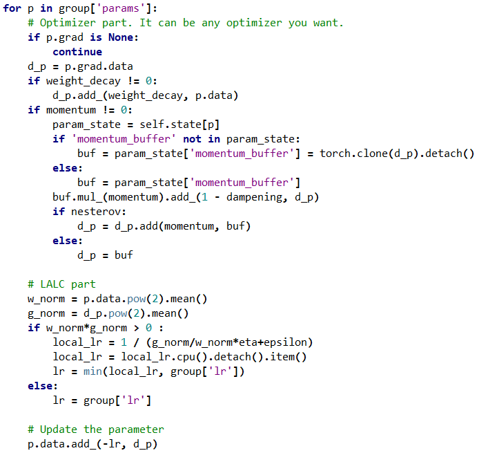
Our proposed algorithm directly embodies these insights. Specifically, we drew from the formula for basic second-order optimization, $\Delta w=(H+\epsilon I)^{-1}J$ , where the Hessian is approximated by the square of the gradient norm. To prevent the scale of the gradient from being affected by the weight norm, we normalized it by the norm of weight. We then established an upper limit for the learning rate using this value. The procedure is detailed in Algorithm 1, and the PyTorch (Paszke et al. 2019) implementation is provided in Appendix B.

Algorithm 1 LALC

w^{l}

: Weight matrix of layer l

\gamma_{t}

: Learning rate at step t

f

: Gradient optimization algorithm (SGD, Adam, etc.)

\eta

\epsilon

: Hyperparameters

while

t<T

for each layer l do

g_{t}^{l}\leftarrow\frac{dL}{dw_{t}^{l}}

m_{t}^{l}\leftarrow f(g^{l},w^{l}_{t})

\lambda^{l}_{t}\leftarrow\frac{1}{\eta||m_{t}^{l}||^{2}/||w_{t}^{l}||^{2}+\epsilon}

w^{l}_{t+1}\leftarrow w^{l}_{t}-min(\gamma_{t},\lambda^{l}_{t})m_{t}^{l}

end while

Figure 5: Our proposed algorithm, inspired by the basic second-order optimization formula. See Section 4 for a detailed explanation, and Appendix B for the PyTorch (Paszke et al. 2019) implementation.

Algorithm	$\Delta W$
Gradient Descent (Baseline)	$\gamma_{t}m_{t}^{l}$
LARS (You et al. 2017)	$\gamma_{t}\frac{\eta\|\|w_{t}^{l}\|\|}{\|\|g_{t}^{l}\|\|+\beta\|\|w_{t}^{l}\|\|+\epsilon}m_{t}^{l}$
LARS/LAMB (You et al. 2019)	$\gamma_{t}\frac{\phi(\|\|w_{t}^{l}\|\|)}{\|\|m_{t}^{l}\|\|+\epsilon}m_{t}^{l}$
LAMBC (Fong et al. 2020)	$\gamma_{t}min\big(\frac{\phi(\|\|w_{t}^{l}\|\|)}{\|\|m_{t}^{l}\|\|+\epsilon},\mu\big)m_{t}^{l}$
CLARS (Huo et al. 2021)	$\gamma_{t}\frac{\eta\|\|w_{t}^{l}\|\|}{\sum_{b}\|\|m_{b,t}^{l}\|\|/B+\epsilon}m_{t}^{l}$
AGC (Brock et al. 2021)	$\gamma_{t}min\big(\frac{\eta\|\|w_{t}^{unit}\|\|}{\|\|m_{t}^{unit}\|\|+\epsilon},1\big)m_{t}^{unit}$
LALC (ours)	$min\Big(\gamma_{t},\frac{1}{\eta\|\|m_{t}^{l}\|\|^{2}/\|\|w_{t}^{l}\|\|^{2}+\epsilon}\Big)m_{t}^{l}$

Table 1: A simple comparison between adaptive rate algorithms, where

\beta

represents the weight decay rate,

\phi

is a ‘scaling function’ as referred to in (You et al. 2019),

\mu

is a clipping hyperparameter, and the rest of the notation follows algorithm 1. Note that CLARS utilizes an average ‘per-sample gradient’ value instead of a minibatch gradient (Huo et al. 2021), and AGC employs a ‘unit-wise ratio’ instead of considering all parameters in each layer. (Brock et al. 2021) For precise definitions and formulations, please refer to the original papers.

5 Experiments

In all of our experiments, we utilized the ResNet50 model (He et al. 2016). For LARS (You et al. 2017), CLARS (Huo et al. 2021), and AGC (Brock et al. 2021), we used a smaller $\eta$ for larger batch sizes. We conducted a hyperparameter search in order of 10, thus careful hyperparameter tuning like (Nado et al. 2021) could potentially enhance performance. LARC and LAMBC was more robust to changes in batch size, possibly due to their clipping-based methodologies. The experimental results are presented in Figure 6 and 7. Please refer to Appendix B for details.

6 Discussion

In this paper, we have investigated the occurrence of gradient explosion in neural network architectures utilizing ReLU activation and batch normalization. Our analysis encompasses a wider range of input and weight distributions; however, our findings may not be fully generalized to practical neural networks. Notably, we have observed that the convolutional layer tends to exhibit a lower explosion rate compared to fully connected layers, as demonstrated in Figure 1. This discrepancy may be attributed to the correlation between activations in convolutional neural networks, where adjacent pixels often exhibit similar activation due to spatial considerations.

References

Abadi et al. (2015) Abadi, M., Agarwal, A., Barham, P., Brevdo, E., Chen, Z., Citro, C., Corrado, G. S., Davis, A., Dean, J., Devin, M., Ghemawat, S., Goodfellow, I., Harp, A., Irving, G., Isard, M., Jia, Y., Jozefowicz, R., Kaiser, L., Kudlur, M., Levenberg, J., Mané, D., Monga, R., Moore, S., Murray, D., Olah, C., Schuster, M., Shlens, J., Steiner, B., Sutskever, I., Talwar, K., Tucker, P., Vanhoucke, V., Vasudevan, V., Viégas, F., Vinyals, O., Warden, P., Wattenberg, M., Wicke, M., Yu, Y., and Zheng, X. TensorFlow: Large-scale machine learning on heterogeneous systems, 2015. URL https://www.tensorflow.org/. Software available from tensorflow.org.
Anwar et al. (2017) Anwar, S., Hwang, K., and Sung, W. Structured pruning of deep convolutional neural networks. ACM Journal on Emerging Technologies in Computing Systems (JETC), 13(3):1–18, 2017.
Ba et al. (2016) Ba, J. L., Kiros, J. R., and Hinton, G. E. Layer normalization. arXiv preprint arXiv:1607.06450, 2016.
Bengio et al. (1994) Bengio, Y., Simard, P., and Frasconi, P. Learning long-term dependencies with gradient descent is difficult. IEEE transactions on neural networks, 5(2):157–166, 1994.
Botev et al. (2016) Botev, A., Lever, G., and Barber, D. Nesterov’s accelerated gradient and momentum as approximations to regularised update descent, 2016. URL https://arxiv.org/abs/1607.01981.
Brock et al. (2021) Brock, A., De, S., Smith, S. L., and Simonyan, K. High-performance large-scale image recognition without normalization. In International Conference on Machine Learning, pp. 1059–1071. PMLR, 2021.
Chatziafratis et al. (2019) Chatziafratis, V., Nagarajan, S. G., Panageas, I., and Wang, X. Depth-width trade-offs for relu networks via sharkovsky’s theorem. arXiv preprint arXiv:1912.04378, 2019.
Chen et al. (2020a) Chen, T., Kornblith, S., Norouzi, M., and Hinton, G. A simple framework for contrastive learning of visual representations. In International conference on machine learning, pp. 1597–1607. PMLR, 2020a.
Chen et al. (2020b) Chen, T., Kornblith, S., Swersky, K., Norouzi, M., and Hinton, G. E. Big self-supervised models are strong semi-supervised learners. Advances in neural information processing systems, 33:22243–22255, 2020b.
Clevert et al. (2015) Clevert, D.-A., Unterthiner, T., and Hochreiter, S. Fast and accurate deep network learning by exponential linear units (elus). arXiv preprint arXiv:1511.07289, 2015.
Dosovitskiy et al. (2020) Dosovitskiy, A., Beyer, L., Kolesnikov, A., Weissenborn, D., Zhai, X., Unterthiner, T., Dehghani, M., Minderer, M., Heigold, G., Gelly, S., et al. An image is worth 16x16 words: Transformers for image recognition at scale. arXiv preprint arXiv:2010.11929, 2020.
Fong et al. (2020) Fong, J., Chen, S., and Chen, K. Improving layer-wise adaptive rate methods using trust ratio clipping. arXiv preprint arXiv:2011.13584, 2020.
Frankle et al. (2020) Frankle, J., Schwab, D. J., and Morcos, A. S. The early phase of neural network training. arXiv preprint arXiv:2002.10365, 2020.
Gilmer et al. (2021) Gilmer, J., Ghorbani, B., Garg, A., Kudugunta, S., Neyshabur, B., Cardoze, D., Dahl, G., Nado, Z., and Firat, O. A loss curvature perspective on training instability in deep learning. arXiv preprint arXiv:2110.04369, 2021.
Goodfellow et al. (2016) Goodfellow, I., Bengio, Y., and Courville, A. Deep learning. MIT press, 2016.
Goyal et al. (2017a) Goyal, P., Dollár, P., Girshick, R., Noordhuis, P., Wesolowski, L., Kyrola, A., Tulloch, A., Jia, Y., and He, K. Accurate, large minibatch sgd: Training imagenet in 1 hour. arXiv preprint arXiv:1706.02677, 2017a.
Goyal et al. (2017b) Goyal, P., Dollár, P., Girshick, R., Noordhuis, P., Wesolowski, L., Kyrola, A., Tulloch, A., Jia, Y., and He, K. Accurate, large minibatch sgd: Training imagenet in 1 hour. arXiv preprint arXiv:1706.02677, 2017b.
Goyal et al. (2017c) Goyal, P., Dollár, P., Girshick, R., Noordhuis, P., Wesolowski, L., Kyrola, A., Tulloch, A., Jia, Y., and He, K. Accurate, large minibatch sgd: Training imagenet in 1 hour. arXiv preprint arXiv:1706.02677, 2017c.
Hastie et al. (2022) Hastie, T., Montanari, A., Rosset, S., and Tibshirani, R. J. Surprises in high-dimensional ridgeless least squares interpolation. The Annals of Statistics, 50(2):949–986, 2022.
He et al. (2015) He, K., Zhang, X., Ren, S., and Sun, J. Delving deep into rectifiers: Surpassing human-level performance on imagenet classification. In Proceedings of the IEEE international conference on computer vision, pp. 1026–1034, 2015.
He et al. (2016) He, K., Zhang, X., Ren, S., and Sun, J. Deep residual learning for image recognition. pp. 770–778, 2016.
Hendrycks & Gimpel (2016) Hendrycks, D. and Gimpel, K. Gaussian error linear units (gelus). arXiv preprint arXiv:1606.08415, 2016.
Huo et al. (2021) Huo, Z., Gu, B., and Huang, H. Large batch optimization for deep learning using new complete layer-wise adaptive rate scaling. In Thirty-Fifth AAAI Conference on Artificial Intelligence, AAAI, pp. 2–9, 2021.
Ioffe & Szegedy (2015) Ioffe, S. and Szegedy, C. Batch normalization: Accelerating deep network training by reducing internal covariate shift. arXiv preprint arXiv:1502.03167, 2015.
Jensen (1906) Jensen, J. L. W. V. Sur les fonctions convexes et les inégalités entre les valeurs moyennes. Acta mathematica, 30(1):175–193, 1906.
Kingma & Ba (2014) Kingma, D. and Ba, J. Adam: A method for stochastic optimization. International Conference on Learning Representations, 12 2014.
Liao & Berg (2018) Liao, J. and Berg, A. Sharpening jensen’s inequality. The American Statistician, 2018.
Lin et al. (2020) Lin, T., Kong, L., Stich, S., and Jaggi, M. Extrapolation for large-batch training in deep learning. In International Conference on Machine Learning, pp. 6094–6104. PMLR, 2020.
Loshchilov & Hutter (2016) Loshchilov, I. and Hutter, F. Sgdr: Stochastic gradient descent with warm restarts. arXiv preprint arXiv:1608.03983, 2016.
Maas et al. (2013) Maas, A. L., Hannun, A. Y., Ng, A. Y., et al. Rectifier nonlinearities improve neural network acoustic models. In Proc. icml, volume 30, pp. 3. Citeseer, 2013.
Mathuriya et al. (2018) Mathuriya, A., Bard, D., Mendygral, P., Meadows, L., Arnemann, J., Shao, L., He, S., Kärnä, T., Moise, D., Pennycook, S. J., et al. Cosmoflow: Using deep learning to learn the universe at scale. In SC18: International Conference for High Performance Computing, Networking, Storage and Analysis, pp. 819–829. IEEE, 2018.
Nado et al. (2021) Nado, Z., Gilmer, J. M., Shallue, C. J., Anil, R., and Dahl, G. E. A large batch optimizer reality check: Traditional, generic optimizers suffice across batch sizes. arXiv preprint arXiv:2102.06356, 2021.
Narayanan et al. (2019) Narayanan, D., Harlap, A., Phanishayee, A., Seshadri, V., Devanur, N. R., Ganger, G. R., Gibbons, P. B., and Zaharia, M. Pipedream: generalized pipeline parallelism for dnn training. In Proceedings of the 27th ACM Symposium on Operating Systems Principles, pp. 1–15, 2019.
Newton (1711) Newton, I. De analysi per aequationes numero terminorum infinitas. 1711.
Pascanu et al. (2013) Pascanu, R., Mikolov, T., and Bengio, Y. On the difficulty of training recurrent neural networks. In International conference on machine learning, pp. 1310–1318. PMLR, 2013.
Paszke et al. (2019) Paszke, A., Gross, S., Massa, F., Lerer, A., Bradbury, J., Chanan, G., Killeen, T., Lin, Z., Gimelshein, N., Antiga, L., Desmaison, A., Kopf, A., Yang, E., DeVito, Z., Raison, M., Tejani, A., Chilamkurthy, S., Steiner, B., Fang, L., Bai, J., and Chintala, S. Pytorch: An imperative style, high-performance deep learning library. In Wallach, H., Larochelle, H., Beygelzimer, A., d'Alché-Buc, F., Fox, E., and Garnett, R. (eds.), Advances in Neural Information Processing Systems 32, pp. 8024–8035. Curran Associates, Inc., 2019. URL http://papers.neurips.cc/paper/9015-pytorch-an-imperative-style-high-performance-deep-learning-library.pdf.
Pennington & Worah (2017) Pennington, J. and Worah, P. Nonlinear random matrix theory for deep learning. Advances in neural information processing systems, 30, 2017.
Philipp et al. (2017) Philipp, G., Song, D., and Carbonell, J. G. The exploding gradient problem demystified-definition, prevalence, impact, origin, tradeoffs, and solutions. arXiv preprint arXiv:1712.05577, 2017.
Qiao et al. (2019) Qiao, S., Wang, H., Liu, C., Shen, W., and Yuille, A. Micro-batch training with batch-channel normalization and weight standardization. arXiv preprint arXiv:1903.10520, 2019.
Ramachandran et al. (2017) Ramachandran, P., Zoph, B., and Le, Q. V. Searching for activation functions. arXiv preprint arXiv:1710.05941, 2017.
Schoenholz et al. (2016) Schoenholz, S. S., Gilmer, J., Ganguli, S., and Sohl-Dickstein, J. Deep information propagation. arXiv preprint arXiv:1611.01232, 2016.
Simonyan & Zisserman (2014) Simonyan, K. and Zisserman, A. Very deep convolutional networks for large-scale image recognition. arXiv preprint arXiv:1409.1556, 2014.
Srivastava et al. (2014) Srivastava, N., Hinton, G., Krizhevsky, A., Sutskever, I., and Salakhutdinov, R. Dropout: a simple way to prevent neural networks from overfitting. The Journal of Machine Learning Research, 15(1):1929–1958, 2014.
Ulyanov et al. (2016) Ulyanov, D., Vedaldi, A., and Lempitsky, V. Instance normalization: The missing ingredient for fast stylization. arXiv preprint arXiv:1607.08022, 2016.
Wu & He (2018) Wu, Y. and He, K. Group normalization. In Proceedings of the European conference on computer vision (ECCV), pp. 3–19, 2018.
Yang et al. (2019) Yang, G., Pennington, J., Rao, V., Sohl-Dickstein, J., and Schoenholz, S. S. A mean field theory of batch normalization. arXiv preprint arXiv:1902.08129, 2019.
You et al. (2017) You, Y., Gitman, I., and Ginsburg, B. Large batch training of convolutional networks. arXiv preprint arXiv:1708.03888, 2017.
You et al. (2019) You, Y., Li, J., Reddi, S., Hseu, J., Kumar, S., Bhojanapalli, S., Song, X., Demmel, J., Keutzer, K., and Hsieh, C.-J. Large batch optimization for deep learning: Training bert in 76 minutes. arXiv preprint arXiv:1904.00962, 2019.
Yousefpour et al. (2021) Yousefpour, A., Shilov, I., Sablayrolles, A., Testuggine, D., Prasad, K., Malek, M., Nguyen, J., Ghosh, S., Bharadwaj, A., Zhao, J., Cormode, G., and Mironov, I. Opacus: User-friendly differential privacy library in PyTorch. arXiv preprint arXiv:2109.12298, 2021.
Yu et al. (2022) Yu, Y., Zhao, Z., Jin, Y., Chen, G., Dou, Q., and Heng, P.-A. Pseudo-label guided cross-video pixel contrast for robotic surgical scene segmentation with limited annotations. arXiv preprint arXiv:2207.09664, 2022.
Zhang et al. (2019) Zhang, H., Dauphin, Y. N., and Ma, T. Fixup initialization: Residual learning without normalization. arXiv preprint arXiv:1901.09321, 2019.
Zhu et al. (2021) Zhu, C., Ni, R., Xu, Z., Kong, K., Huang, W. R., and Goldstein, T. Gradinit: Learning to initialize neural networks for stable and efficient training. Advances in Neural Information Processing Systems, 34:16410–16422, 2021.

Appendix A Appendix

A.1 Proof of Proposition 2.1

We use the moment generating function and its properties.

$\displaystyle M_{X}(t):$	$\displaystyle=\mathbb{E}[e^{tX}]$	(8)
	$\displaystyle=e^{0}P(X=0)+\int^{\infty}_{0}e^{tx}\frac{1}{\sqrt{2\pi}\sigma}e^{-\frac{(x-\mu)^{2}}{2\sigma^{2}}}dx$
	$\displaystyle=P(N(\mu,\sigma^{2})\leq 0)+\int^{\infty}_{0}\frac{1}{\sqrt{2\pi}\sigma}e^{-\frac{(x-\mu-\sigma^{2}t)^{2}-2\mu\sigma^{2}t-\sigma^{4}t^{2}}{2\sigma^{2}}}dx$
	$\displaystyle=\phi(-\frac{\mu}{\sigma})+e^{\mu t+\frac{\sigma^{2}t^{2}}{2}}\int^{\infty}_{0}\frac{1}{\sqrt{2\pi}\sigma}e^{-\frac{(x-\mu-\sigma^{2}t)^{2}}{2\sigma^{2}}}dx$

where $\phi(x)=\int_{-\infty}^{x}\frac{1}{\sqrt{2\pi}}e^{-x^{2}/2}$ is the cumulative distribution function of the standard normal distribution. Substituting $x^{\prime}=(x-\mu-\sigma^{2}t)/\sigma$ ,

		$\displaystyle=\phi(-\frac{\mu}{\sigma})+e^{\mu t+\frac{\sigma^{2}t^{2}}{2}}\int^{\infty}_{-\frac{\mu+\sigma^{2}t}{\sigma}}\frac{1}{\sqrt{2\pi}}e^{-\frac{x^{\prime 2}}{2}}dx^{\prime}$		(9)
		$\displaystyle=\phi(-\frac{\mu}{\sigma})+e^{\mu t+\frac{\sigma^{2}t^{2}}{2}}(1-\phi(-\frac{\mu+\sigma^{2}t}{\sigma}))$		(9)

We calculate the first and second moment from the moment generating function.

$\displaystyle\frac{d}{dt}M_{X}(t)$	$\displaystyle=(\mu+\sigma^{2}t)e^{\mu t+\frac{\sigma^{2}t^{2}}{2}}(1-\phi(-\frac{\mu+\sigma^{2}t}{\sigma}))+e^{\mu t+\frac{\sigma^{2}t^{2}}{2}}(-1)(-\sigma)\frac{1}{\sqrt{2\pi}}e^{-\frac{1}{2}(\frac{\mu+\sigma^{2}t}{\sigma})^{2}}$	(10)
	$\displaystyle=(\mu+\sigma^{2}t)e^{\mu t+\frac{\sigma^{2}t^{2}}{2}}(1-\phi(-\frac{\mu+\sigma^{2}t}{\sigma}))+\frac{\sigma}{\sqrt{2\pi}}e^{-\frac{\mu^{2}+2\mu\sigma^{2}t+\sigma^{4}t^{2}-2\sigma^{2}(\mu t+\sigma^{2}t^{2}/2)}{2\sigma^{2}}}$
	$\displaystyle=(\mu+\sigma^{2}t)e^{\mu t+\frac{\sigma^{2}t^{2}}{2}}(1-\phi(-\frac{\mu+\sigma^{2}t}{\sigma}))+\frac{\sigma}{\sqrt{2\pi}}e^{-\frac{\mu^{2}}{2\sigma^{2}}}$

$\displaystyle\frac{d^{2}}{dt^{2}}M_{X}(t)$	$\displaystyle=(\sigma^{2}+(\mu+\sigma^{2}t)^{2})e^{\mu t+\frac{\sigma^{2}t^{2}}{2}}(1-\phi(-\frac{\mu+\sigma^{2}t}{\sigma}))$	(11)
	$\displaystyle+(\mu+\sigma^{2}t)\ e^{\mu t+\frac{\sigma^{2}t^{2}}{2}}\frac{d}{dt}[1-\phi(-\frac{\mu+\sigma^{2}t}{\sigma})]$
	$\displaystyle=(\sigma^{2}+(\mu+\sigma^{2}t)^{2})e^{\mu t+\frac{\sigma^{2}t^{2}}{2}}(1-\phi(-\frac{\mu+\sigma^{2}t}{\sigma}))+(\mu+\sigma^{2}t)\frac{\sigma}{\sqrt{2\pi}}e^{-\frac{\mu^{2}}{2\sigma^{2}}}$

Now, we finally obtain:

\displaystyle\mathbb{E}(X)

\displaystyle=\frac{d}{dt}M_{X}(t)|_{t=0}=\mu(1-\phi(-\frac{\mu}{\sigma}))+\frac{\sigma}{\sqrt{2\pi}}e^{-\frac{\mu^{2}}{2\sigma^{2}}}

(12)

	$\displaystyle\mathrm{Var}(X)$	$\displaystyle=\frac{d^{2}}{dt^{2}}M_{X}(t)\|_{t=0}-(\frac{d}{dt}M_{X}(t)\|_{t=0})^{2}$		(13)
		$\displaystyle=(\sigma^{2}+\mu^{2})(1-\phi(-\frac{\mu}{\sigma}))+\mu\frac{\sigma}{\sqrt{2\pi}}e^{-\frac{\mu^{2}}{2\sigma^{2}}}-(\mu(1-\phi(-\frac{\mu}{\sigma}))+\frac{\sigma}{\sqrt{2\pi}}e^{-\frac{\mu^{2}}{2\sigma^{2}}})^{2}$		(13)

which proves the proposition.

A.2 Proof of Theorem 2.2

Let us denote $\mathrm{ReLU}(x^{n})=x^{n+}$ , $W^{n}x^{n+}+b^{n}=\hat{x}^{n+1}$ , and $BatchNorm(\hat{x}^{n+1})=x^{n+1}$ . We first calculate the statistics of $\hat{x}^{n+1}$ , which is estimated by the batch normalization layer.

$\displaystyle\hat{\mu}_{j}^{n+1}$	$\displaystyle=\mathbb{E}_{x}[\hat{x}^{n+1}_{j}]$	(14)
	$\displaystyle=\mathbb{E}_{x}[\sum_{i}(x^{n+}_{i}W^{n}_{ij})+b^{n}_{j}]$
	$\displaystyle=\sum_{i}(\mathbb{E}_{x}[x^{n+}_{i}]W^{n}_{ij})+b^{n}_{j}$
	$\displaystyle=\sum_{i}(\mu^{n}(1-\phi(-\frac{\mu^{n}}{\sigma^{n}}))+\frac{\sigma^{n}}{\sqrt{2\pi}}e^{-\frac{(\mu^{n})^{2}}{2(\sigma^{n})^{2}}})W^{n}_{ij}+b^{n}_{j}$

Note that this equation describes the sampling process of the batch normalization layer, therefore the statistics of model parameters( $W^{n}_{ij}$ , $b^{n}_{j}$ ) are not considered. Other than this part, we omit the subscript if obvious. Similarly,

$\displaystyle(\hat{\sigma}_{j}^{n+1})^{2}$	$\displaystyle=Var_{x}(\hat{x}^{n+1}_{j})$	(15)
	$\displaystyle=Var_{x}(\sum_{i}(x^{n+}_{i}W^{n}_{ij})+b^{n}_{j})$
	$\displaystyle=\sum_{i}Var_{x}(x^{n+}_{i}W^{n}_{ij})$
	$\displaystyle=\sum_{i}(W^{n}_{ij})^{2}Var_{x}(x^{n+}_{i})$
	$\displaystyle=(((\sigma^{n})^{2}+(\mu^{n})^{2})(1-\phi(-\frac{\mu^{n}}{\sigma^{n}}))+\mu^{n}\frac{\sigma^{n}}{\sqrt{2\pi}}e^{-\frac{(\mu^{n})^{2}}{2(\sigma^{n})^{2}}}$
	$\displaystyle-(\mu^{n}(1-\phi(-\frac{\mu^{n}}{\sigma^{n}}))+\frac{\sigma^{n}}{\sqrt{2\pi}}e^{-\frac{(\mu^{n})^{2}}{2(\sigma^{n})^{2}}})^{2})\sum_{i}(W^{n}_{ij})^{2}$

And $x^{n+1}_{j}$ is given by:

	$\displaystyle x^{n+1}_{j}$	$\displaystyle=BatchNorm(\hat{x}^{n+1})$		(16)
		$\displaystyle=\frac{\hat{x}^{n+1}-\hat{\mu}_{j}^{n+1}}{\hat{\sigma}_{j}^{n+1}}\gamma^{n+1}_{j}+\beta^{n+1}_{j}$		(16)

where $\gamma^{n+1},\beta^{n+1}\in\mathbb{R}^{n_{d+1}}$ are affine transform parameters of batch normalization.

Now, we calculate the gradient of the input using the backpropagation algorithm. Since ReLU operation not only changes the activation but also blocks the gradient, they are treated separately. For indices such that $x^{n}_{i}\leq 0$ , the gradient $g^{n}_{i}$ is just zero. Then, for each $i$ that is not blocked by ReLU (i.e. for $i\in\{i:x^{n}_{i}>0\}$ ), we have:

$\displaystyle g_{i}^{n}$	$\displaystyle=\frac{dL}{dx^{n}_{i}}=\sum_{j}\frac{dL}{dx^{n+1}_{j}}\frac{dx^{n+1}_{j}}{dx^{n}_{i}}$	(17)
	$\displaystyle=\sum_{j}g^{n+1}_{j}\frac{dx^{n+1}_{j}}{d\hat{x}^{n+1}_{j}}\frac{d\hat{x}^{n+1}_{j}}{dx^{n}_{i}}$
	$\displaystyle=\sum_{j}g^{n+1}_{j}\frac{\gamma^{n+1}_{j}}{\hat{\sigma}_{j}^{n+1}}W^{n}_{ij}$

Assuming the gradient $g^{n+1}_{j}$ is zero-centered and independent to other variables, we have

$\displaystyle\mathrm{Var}(g_{i}^{n})$	$\displaystyle=\mathrm{Var}(\sum_{j}g^{n+1}_{j}\frac{\gamma^{n+1}_{j}}{\hat{\sigma}^{n+1}_{j}}W^{n}_{ij})$	(18)
	$\displaystyle=\sum_{j}\mathrm{Var}(g^{n+1}_{j}\frac{\gamma^{n+1}_{j}}{\hat{\sigma}^{n+1}_{j}}W^{n}_{ij})$
	$\displaystyle=\sum_{j}\mathbb{E}[(g^{n+1}_{j}\frac{\gamma^{n+1}_{j}}{\hat{\sigma}^{n+1}_{j}}W^{n}_{ij})^{2}]-\mathbb{E}[g^{n+1}_{j}\frac{\gamma^{n+1}_{j}}{\hat{\sigma}^{n+1}_{j}}W^{n}_{ij}]^{2}$
	$\displaystyle=\sum_{j}\mathrm{Var}(g^{n+1}_{j})(\gamma^{n+1}_{j})^{2}\mathbb{E}[\frac{1}{(\hat{\sigma}^{n+1}_{j})^{2}}]\mathbb{E}[(W^{n}_{ij})^{2}]$

since $f(x)=1/x$ is convex at $x>0$ , we can apply Jensen’s inequality (Jensen 1906).

		$\displaystyle\geq\sum_{j}\mathrm{Var}(g^{n+1}_{j})(\gamma^{n+1}_{j})^{2}\frac{1}{\mathbb{E}[(\hat{\sigma}^{n+1}_{j})^{2}]}\mathbb{E}[(W^{n}_{ij})^{2}]$		(19)
		$\displaystyle=\sum_{j}\mathrm{Var}(g^{n+1}_{j})(\sigma^{n+1}_{j})^{2}\frac{\mathbb{E}[(W^{n}_{ij})^{2}]}{\mathbb{E}[\sum_{k}\mathrm{Var}(x_{k}^{n+})(W^{n}_{kj})^{2}]}$
		$\displaystyle=\sum_{j}(\sigma^{n+1}_{j})^{2}\mathrm{Var}(g^{n+1}_{j})\frac{\sigma_{w}^{2}}{\mathbb{E}[\sum_{k}\mathrm{Var}(x_{k}^{n+})]\sigma_{w}^{2}}$
		$\displaystyle=\frac{1}{\sum_{k}\mathrm{Var}(x_{k}^{n+})}\sum_{j}(\sigma^{n+1}_{j})^{2}\mathrm{Var}(g^{n+1}_{j})$

The equality holds when $\hat{\sigma}_{j}^{n+1}$ is identical for all $j$ . Note that this formula is no longer dependent on the input index $i$ , if $x_{i}^{n}$ is not blocked by ReLU. Since the probability of passing ReLU is $1-\phi(-\mu^{n}/\sigma^{n})$ for any input index $i$ , we have

$\displaystyle\mathbb{E}$	$\displaystyle[\sum_{i}(\sigma_{i}^{n})^{2}\mathrm{Var}(g^{n}_{i})]/\sum_{j}(\sigma^{n+1}_{j})^{2}\mathrm{Var}(g_{j}^{n+1})]$	(20)
	$\displaystyle\geq\mathbb{E}[\sum_{i}(1-\phi(-\frac{\mu^{n}}{\sigma^{n}}))(\sigma^{n})^{2}\frac{1}{\sum_{k}\mathrm{Var}(x_{k}^{n+})}\sum_{j}(\sigma^{n+1}_{j})^{2}\mathrm{Var}(g^{n+1}_{j})/\sum_{j}(\sigma^{n+1}_{j})^{2}\mathrm{Var}(g_{j}^{n+1})]$
	$\displaystyle=(1-\phi(-\frac{\mu^{n}}{\sigma^{n}}))(\sigma^{n})^{2}/\Big(((\sigma^{n})^{2}+(\mu^{n})^{2})(1-\phi(-\frac{\mu^{n}}{\sigma^{n}}))+\mu^{n}\frac{\sigma^{n}}{\sqrt{2\pi}}e^{-\frac{(\mu^{n})^{2}}{2(\sigma^{n})^{2}}}$
	$\displaystyle-(\mu^{n}(1-\phi(-\frac{\mu^{n}}{\sigma^{n}}))+\frac{\sigma^{n}}{\sqrt{2\pi}}e^{-\frac{(\mu^{n})^{2}}{2(\sigma^{n})^{2}}})^{2}\Big)$
	$\displaystyle=\frac{1-\phi(-\frac{\mu^{n}}{\sigma^{n}})}{(1+(\frac{\mu^{n}}{\sigma^{n}})^{2})(1-\phi(-\frac{\mu^{n}}{\sigma^{n}}))+\frac{\mu^{n}}{\sigma^{n}}\frac{1}{\sqrt{2\pi}}exp(-\frac{1}{2}(\frac{\mu^{n}}{\sigma^{n}})^{2})-(\frac{\mu^{n}}{\sigma^{n}}(1-\phi(-\frac{\mu^{n}}{\sigma^{n}}))+\frac{1}{\sqrt{2\pi}}exp(-\frac{1}{2}(\frac{\mu^{n}}{\sigma^{n}})^{2}))^{2}}$
	$\displaystyle=\frac{\erfc(-R)}{(1+2R^{2})\erfc(-R)+2Re^{-R^{2}}/\sqrt{\pi}-(R\erfc(-R)+e^{-R^{2}}/\sqrt{\pi})^{2}}$

where $R:=\frac{\mu^{n}}{\sqrt{2}\sigma^{n}}$ and $\erfc(x)=\frac{2}{\pi}\int_{x}^{\infty}\frac{1}{\sqrt{2\pi}}e^{-x^{2}/2}=2-2\phi(x\sqrt{2})$ is a complementary error function.

A.3 Proof of Corollary 2.3

In case of $R\to-\infty$ , observing $\erfc(x)$ exponentially converges to zero at $x\to\infty$ , both denominator and numerator converges to zero. And the derivative of the denominator

$\displaystyle\frac{d}{dR}$	$\displaystyle\Big((1+2R^{2})\erfc(-R)+2R\frac{e^{-R^{2}}}{\sqrt{\pi}}-(R\erfc(-R)+\frac{e^{-R^{2}}}{\sqrt{\pi}})^{2}\Big)$	(21)
	$\displaystyle=4R\erfc(-R)+(1+2R^{2})2\frac{e^{-R^{2}}}{\sqrt{\pi}}+(2-4R^{2})\frac{e^{-R^{2}}}{\sqrt{\pi}}$
	$\displaystyle-2(R\erfc(-R)+\frac{e^{-R^{2}}}{\sqrt{\pi}})(\erfc(-R)+R\cdot 2\frac{e^{-R^{2}}}{\sqrt{\pi}}-2R\frac{e^{-R^{2}}}{\sqrt{\pi}})$
	$\displaystyle=4R\erfc(-R)+\frac{e^{-R^{2}}}{\sqrt{\pi}}(4-2\erfc(-R))-2R\erfc(-R)^{2}$
	$\displaystyle=2(2-\erfc(-R))(\erfc(-R)+\frac{e^{-R^{2}}}{\sqrt{\pi}})$

is strictly positive in $(-\infty,\infty)$ . Therefore we can utilize L’Hôpital’s rule:

$\displaystyle\lim_{R\to-\infty}$	$\displaystyle\frac{\erfc(-R)}{(1+2R^{2})\erfc(-R)+2Re^{-R^{2}}/\sqrt{\pi}-(R\erfc(-R)+e^{-R^{2}}/\sqrt{\pi})^{2}}$	(22)
	$\displaystyle=\lim_{R\to-\infty}\frac{\frac{e^{-R^{2}}}{\sqrt{\pi}}}{(2-\erfc(-R))(\erfc(-R)+\frac{e^{-R^{2}}}{\sqrt{\pi}})}$
	$\displaystyle=\lim_{R\to-\infty}\frac{1}{(2-\erfc(-R))(\erfc(-R)/(\frac{e^{-R^{2}}}{\sqrt{\pi}})+1)}=\infty$

since $2-\erfc(-R)\to 0+$ and $\erfc(-R)/e^{-R^{2}}\to 0$ .

(23)

A.4 Proof of Theorem 2.4

We start from eq.(17) and get the upper bound of $\mathbb{E}[1/(\hat{\sigma}_{j}^{n+1})^{2}]$ instead of lower bound. Since $W_{ij}$ is normally distributed, $\sum W_{ij}$ can be viewed as a noncentral chi-squared distribution with nontrivial variance. Let $X$ be a chi-squared distribution with $d_{n}$ degrees of freedom. For any $0<c<1$ and $t<0$ ,

	$\displaystyle P(\sum_{i}(\frac{W_{ij}^{n}}{\sigma_{w}})^{2}<d_{n}\delta)$	$\displaystyle\leq P(X<d_{n}\delta)=P(e^{tX}>d_{n}t\delta)$		(24)
		$\displaystyle\leq M_{X}(t)e^{-t\delta n}=e^{-(n/2)ln(1-2t)-t\delta n}$		(24)

The first inequality comes from the fact that $W_{ij}/\sigma_{w}$ may not be zero-centered, and the second one is Markov’s inequality. Setting $t=(1-1/\delta)/2$ ,

\displaystyle P(\sum_{i}(W_{ij}^{n})^{2}<\sigma_{w}^{2}d_{n}\delta)

\displaystyle\leq e^{-(d_{n}/2)(\delta-1-\mathrm{ln}(\delta))}

(25)

Using the sharpened Jensen’s inequality $\mathbb{E}[f(X)]-f(\mathbb{E}[X])\leq\sigma^{2}_{X}\mathrm{sup}(f^{\prime\prime}(x)/2)$ proposed by (Liao & Berg 2018), at least with probability $1-e^{-(d_{n}/2)(\delta-1-\mathrm{ln}(\delta))}$ , we have

$\displaystyle\mathbb{E}[\frac{1}{\hat{\sigma}_{j}^{n+1}}]\mathbb{E}[(W_{ij}^{n})^{2}]$	$\displaystyle=\frac{1}{\sum_{k}\mathrm{Var}(x_{k}^{n+})}\mathbb{E}[\frac{1}{(W_{ij}^{n})^{2}}]\mathbb{E}[(W_{ij}^{n})^{2}]$	(26)
	$\displaystyle\leq\frac{1}{\sum_{k}\mathrm{Var}(x_{k}^{n+})}(\frac{\mathbb{E}[(W_{ij}^{n})^{2}]}{\mathbb{E}[(W_{ij}^{n})^{2}]}+\mathbb{E}[(W_{ij}^{n})^{2}]2\sigma_{w}^{4}(1+2\frac{\mu_{w}^{2}}{\sigma_{w}^{2}})\frac{2}{2(\sigma_{w}^{2}d_{n}\delta)^{3}})$
	$\displaystyle=\frac{1}{\sum_{k}\mathrm{Var}(x_{k}^{n+})}(1+\sigma_{w}^{2}(1+\frac{\mu_{w}^{2}}{\sigma_{w}^{2}})\sigma_{w}^{4}(1+2\frac{\mu_{w}^{2}}{\sigma_{w}^{2}})\frac{2}{\sigma_{w}^{6}d_{n}^{3}\delta^{3}})$
	$\displaystyle=\frac{1}{\sum_{k}\mathrm{Var}(x_{k}^{n+})}(1+\frac{2(1+\frac{\mu_{w}^{2}}{\sigma_{w}^{2}})(1+2\frac{\mu_{w}^{2}}{\sigma_{w}^{2}})}{d_{n}^{3}\delta^{3}})$

There is at least $(1-\mathrm{exp}(-(d_{n}/2)(\delta-1-\mathrm{ln}(\delta))))^{d_{n+1}}\geq 1-d_{n+1}\mathrm{exp}(-(d_{n}/2)(\delta-1-\mathrm{ln}(\delta)))$ chance that the inequality holds for all $1\leq j\leq d_{n+1}$ . The remaining part is the same as Theorem 2.2.

A.5 Proof of Theorem 2.8

Since inputs( $x^{n}$ ) are perfectly correlated, let $b\sim N(0,1)$ and $x^{n}=bt$ , where $t\in\mathbb{R}^{n_{d}}$ is treated as a constant. Similar to Theorem 1, We denote $\mathrm{ReLU}(x^{n})=x^{n+}$ , $W^{n}x^{n+}+b^{n}=\hat{x}^{n+1}$ , and $BatchNorm(\hat{x}^{n+1})=x^{n+1}$ but ignore the bias term $b^{n}$ since it doesn’t affect the variance and is immediately normalized by the batch normalization layer. We first calculate the mean and variance of $\hat{x}^{n+1}$ . As the sign of $x^{n}$ is reversed corresponding to positive and negative $t$ , they are treated separately.

$\displaystyle\hat{\mu}_{j}^{n+1}$	$\displaystyle=\mathbb{E}_{x}[\hat{x}^{n+1}_{j}]$	(27)
	$\displaystyle=\mathbb{E}_{x}[\hat{x}^{n+1}_{j}\|b\geq 0]P(b\geq 0)+E_{x}[\hat{x}^{n+1}_{j}\|b\leq 0]P(b\leq 0)$
	$\displaystyle=\frac{1}{2}\mathbb{E}_{x}[\sum_{i}W_{ij}^{n}\mathrm{ReLU}(t_{i})b\|b\geq 0]+\frac{1}{2}E_{x}[\sum_{i}W_{ij}^{n}\mathrm{ReLU}(-t_{i})(-b)\|b\leq 0]$
	$\displaystyle=\frac{1}{2}\frac{2}{\sqrt{2\pi}}\sum_{i}W_{ij}^{n}(\mathrm{ReLU}(t_{i})+\mathrm{ReLU}(-t_{i}))$
	$\displaystyle=\frac{1}{\sqrt{2\pi}}\sum_{i}W_{ij}^{n}\|t_{i}\|$

The conditional expectation of $b$ is calculated using Proposition 1. Then, we directly calculate the variance before normalization.

$\displaystyle(\hat{\sigma}_{j}^{n+1})^{2}$	$\displaystyle=\int_{-\infty}^{\infty}(\hat{x}^{n+1}_{j}-\hat{\mu}_{j}^{n+1})^{2}P(b)db$	(28)
	$\displaystyle=\int_{-\infty}^{0}(\sum_{i}W_{ij}^{n}\mathrm{ReLU}(-t_{i})(-b)-\hat{\mu}_{j}^{n+1})^{2}\frac{1}{\sqrt{2\pi}}e^{-\frac{b^{2}}{2}}db$
	$\displaystyle+\int_{0}^{\infty}(\sum_{i}W_{ij}^{n}\mathrm{ReLU}(t_{i})(b)-\hat{\mu}_{j}^{n+1})^{2}\frac{1}{\sqrt{2\pi}}e^{-\frac{b^{2}}{2}}db$
	$\displaystyle=\int_{-\infty}^{0}(-N_{j}b-\hat{\mu}_{j}^{n+1})^{2}\frac{1}{\sqrt{2\pi}}e^{-\frac{b^{2}}{2}}db+\int_{0}^{\infty}(P_{j}b-\hat{\mu}_{j}^{n+1})^{2}\frac{1}{\sqrt{2\pi}}e^{-\frac{b^{2}}{2}}db$

where $N_{j}:=\sum_{i}W_{ij}^{n}\mathrm{ReLU}(-t_{i})$ and $P_{j}:=\sum_{i}W_{ij}^{n}\mathrm{ReLU}(t_{i})$ . Using the formula $\int(ax-b)^{2}e^{-x^{2}/2}dx=\sqrt{\frac{\pi}{2}}(a^{2}+b^{2})erf(\frac{x}{\sqrt{2}})-ae^{-x^{2}/2}(ax-2b)+C$ , where $erf(x)=2\phi(x\sqrt{2})-1$ is an error function, we obtain:

		$\displaystyle=\frac{1}{\sqrt{2\pi}}\Big[\sqrt{\frac{\pi}{2}}(N_{j}^{2}+(\hat{\mu}_{j}^{n+1})^{2})erf(\frac{x}{\sqrt{2}})+Ne^{-\frac{x^{2}}{2}}(-N_{j}x-2\hat{\mu}_{j}^{n+1})\Big]^{0}_{-\infty}$		(29)
		$\displaystyle+\frac{1}{\sqrt{2\pi}}\Big[\sqrt{\frac{\pi}{2}}(P_{j}^{2}+(\hat{\mu}_{j}^{n+1})^{2})erf(\frac{x}{\sqrt{2}})-Pe^{-\frac{x^{2}}{2}}(P_{j}x-2\hat{\mu}_{j}^{n+1})\Big]^{\infty}_{0}$
		$\displaystyle=\frac{1}{\sqrt{2\pi}}[-2N_{j}\hat{\mu}_{j}^{n+1}+\sqrt{\frac{\pi}{2}}(N_{j}^{2}+(\hat{\mu}_{j}^{n+1})^{2})+\sqrt{\frac{\pi}{2}}(P_{j}^{2}+(\hat{\mu}_{j}^{n+1})^{2})-2P_{j}\hat{\mu}_{j}^{n+1}]$
		$\displaystyle=\frac{1}{2}(N_{j}^{2}+P_{j}^{2})+(\hat{\mu}_{j}^{n+1})^{2}-\sqrt{\frac{2}{\pi}}\hat{\mu}_{j}^{n+1}(P_{j}+N_{j})$

Since $\{W_{ij}\}$ are independent of each other and $\mathbb{E}[N_{j}]=\mathbb{E}[P_{j}]=\mathbb{E}[\hat{\mu}_{j}^{n+1}]=0$ , we obtain:

$\displaystyle\mathbb{E}[(\hat{\sigma}_{j}^{n+1})^{2}]$	$\displaystyle=\mathbb{E}[\frac{1}{2}(N_{j}^{2}+P_{j}^{2})+(\mu_{j}^{n+1})^{2}-\sqrt{\frac{2}{\pi}}\mu_{j}^{n+1}(P_{j}+N_{j})]$	(30)
	$\displaystyle=\frac{1}{2}(\mathbb{E}[N_{j}^{2}]+\mathbb{E}[P_{j}^{2}])+\mathbb{E}[(\mu_{j}^{n+1})^{2}]-\sqrt{\frac{2}{\pi}}\mathbb{E}[\mu_{j}^{n+1}(P_{j}+N_{j})]$
	$\displaystyle=\frac{1}{2}(\mathrm{Var}(N_{j})+\mathrm{Var}(P_{j}))+\mathrm{Var}(\mu_{j}^{n+1})-0$
	$\displaystyle=\frac{1}{2}(\sigma_{w}^{2}\sum_{i}\mathrm{ReLU}(t_{i})^{2}+\sigma_{w}^{2}\sum_{i}\mathrm{ReLU}(-t_{i})^{2})+\frac{1}{2\pi}\sigma_{w}^{2}\sum_{i}\|t_{i}\|^{2}$
	$\displaystyle=\sigma_{w}^{2}(\frac{1}{2}+\frac{1}{2\pi})\sum_{i}t_{i}^{2}$

where $\sigma_{w}$ denotes the standard deviation of the weight. Let $I^{+}:=\{i:x^{n}_{i}>0\}$ . For $i\in I^{+}$ , we have:

$\displaystyle\mathrm{Var}(g_{i}^{n})$	$\displaystyle=\mathrm{Var}(\sum_{j}g^{n+1}_{j}\frac{\gamma^{n+1}_{j}}{\hat{\sigma}^{n+1}_{j}}W^{n}_{ij})$	(31)
	$\displaystyle=\sum_{j}\mathrm{Var}(g^{n+1}_{j}\frac{\gamma^{n+1}_{j}}{\hat{\sigma}^{n+1}_{j}}W^{n}_{ij})$
	$\displaystyle=\sum_{j}\mathrm{Var}(g^{n+1}_{j})(\mathbb{E}[\frac{\gamma_{j}^{2}}{(\hat{\sigma}^{n+1}_{j})^{2}}(W^{n}_{ij})^{2}]-\mathbb{E}[\frac{\gamma^{n+1}_{j}}{\sigma^{n+1}_{j}}W^{n}_{ij}]^{2})$
	$\displaystyle=\sum_{j}\mathrm{Var}(g^{n+1}_{j})(\gamma^{n+1}_{j})^{2}\mathbb{E}[\frac{1}{(\hat{\sigma}^{n+1}_{j})^{2}}]\mathbb{E}[(W^{n}_{ij})^{2}]$
	$\displaystyle\geq\sum_{j}\mathrm{Var}(g^{n+1}_{j})(\gamma^{n+1}_{j})^{2}\frac{1}{\mathbb{E}[(\hat{\sigma}^{n+1}_{j})^{2}]}\mathbb{E}[(W^{n}_{ij})^{2}]$
	$\displaystyle=\frac{2\pi}{\pi+1}\sum_{j}(\sigma^{n+1}_{j})^{2}\mathrm{Var}(g^{n+1}_{j})\frac{\sigma_{w}^{2}}{\sum_{k}t_{k}^{2}\sigma_{w}^{2}}$
	$\displaystyle=\frac{2\pi}{\pi+1}\frac{1}{\sum_{k}t_{k}^{2}}\sum_{j}(\sigma^{n+1}_{j})^{2}\mathrm{Var}(g^{n+1}_{j})$

The equality holds when $\hat{\sigma}_{j}^{n+1}$ are identical for all $j$ . Finally, we obtain:

$\displaystyle\mathbb{E}$	$\displaystyle[\sum_{i}(\sigma_{i}^{n})^{2}\mathrm{Var}(g^{n}_{i})/\sum_{j}(\sigma^{n+1}_{j})^{2}\mathrm{Var}(g^{n+1}_{j})]$	(32)
	$\displaystyle\geq\mathbb{E}[\frac{1}{2}\sum_{i}t_{i}^{2}\frac{2\pi}{\pi+2}\frac{1}{\sum_{k}t_{k}^{2}}\sum_{j}(\sigma^{n+1}_{j})^{2}\mathrm{Var}(g^{n+1}_{j})/\sum_{j}(\sigma^{n+1}_{j})^{2}\mathrm{Var}(g^{n+1}_{j})]$
	$\displaystyle=\frac{1}{2}\frac{2\pi}{\pi+1}\frac{\sum_{i}t_{i}^{2}}{\sum_{k}t_{k}^{2}}$
	$\displaystyle=\frac{\pi}{\pi+1}$

This proves the theorem.

A.6 Proof of Lemma 2.9

Let $x^{N}$ be an output of the network, which is scalar by definition. Since a ReLU network is piecewise linear, $dx^{N}/dx_{i}^{n}$ is not a function of $x_{i}^{n}$ , for arbitrary $n\leq N$ and $i\leq d_{n}$ . Let $l$ be a nonlinear loss function and $L=l(dx^{N})$ .

\displaystyle h_{i}^{n}:=\frac{d^{2}L}{(dx_{i}^{n})^{2}}

\displaystyle=\frac{d^{2}l(x^{N})}{(dx_{i}^{n})^{2}}=\frac{d}{dx_{i}^{n}}\Big(\frac{dx^{N}}{dx_{i}^{n}}l^{\prime}(x^{N})\Big)=\Big(\frac{dx^{N}}{dx_{i}^{n}}\Big)^{2}l^{\prime\prime}(x^{N})=\Big(\frac{g_{i}^{n}}{l^{\prime}(x^{N})}\Big)^{2}l^{\prime\prime}(x^{N})

(33)

If $g$ is normally distributed, statistics of $h$ can be calculated with a chi-square distribution with $1$ degree of freedom.

\displaystyle\frac{\mathrm{Var}(h_{i}^{n})}{\mathrm{Var}(h_{j}^{m})}

\displaystyle=\frac{\frac{l^{\prime\prime}(x^{N})^{2}}{l^{\prime}(x^{N})^{4}}\mathrm{Var}((g_{i}^{n})^{2})}{\frac{l^{\prime\prime}(x^{N})^{2}}{l^{\prime}(x^{N})^{4}}\mathrm{Var}((g_{j}^{m})^{2})}=\frac{\mathrm{Var}(g_{i}^{n})^{2}2\cdot 1}{\mathrm{Var}(g_{j}^{m})^{2}2\cdot 1}=\Big(\frac{\mathrm{Var}(g_{i}^{n})}{\mathrm{Var}(g_{j}^{m})}\Big)^{2}

(34)

Appendix B Experimental Details

In all experiments, we employed Stochastic Gradient Descent with a momentum of 0.9 and weight decay rate of $5\times 10^{-4}$ . We employed a learning rate of $0.1$ for a batch size of $128$ , which was then linearly scaled with batch size. (Goyal et al. 2017a) For the CIFAR10 experiment, we utilized the ResNet50 architecture (He et al. 2016). To accommodate the smaller image size, we removed the first pooling layer and stride operation of the first convolutional layer. The input images were normalized using the mean values of (0.4914, 0.4822, 0.4465) and standard deviation values of (0.2023, 0.1994, 0.2010). Random cropping with a padding size of 4 and random horizontal flips were applied as data augmentation techniques. In the case of using WarmUp (Goyal et al. 2017b), the learning rate was linearly increased over the first 10 epochs for the CIFAR10 experiment (20 or 30 epochs for a ‘longer’ WarmUp) and two epochs for the ImageNet experiment. Subsequently, a cosine learning rate decay without restarts (Loshchilov & Hutter 2016) was employed.

In the ImageNet experiment, the input images were normalized using the mean values of (0.485, 0.456, 0.406) and standard deviation values of (0.229, 0.224, 0.225). As data augmentation, we applied RandomResizedCrop (He et al. 2016) with an image size of 224, followed by a random horizontal flip. During the evaluation step, the images were resized to a size of 256 and center-cropped to a size of 224.

All experiments were conducted using a single RTX2080 Ti 12GB GPU. For experiments with large batch sizes, we utilized a computational trick where the parameter update was performed every n steps to effectively increase the batch size by n times. This approach is almost identical to using a batch size that is n times larger, with the exception of slightly higher sampling errors from normalization layers.

LAMB (You et al. 2019), a modified version of LARS based on the Adam optimizer (Kingma & Ba 2014), was not considered in these experiments. The Adam optimizer requires an additional hyperparameter and exhibits different characteristics, making a fair comparison with an SGD optimizer more complex. While Adam is known for its fast convergence, a basic SGD optimizer with momentum often outperforms it when employing a longer training schedule. Although the entire experiment could be repeated using an Adam-family optimizer, we do not consider it necessary at this time.

Nesterov momentum (Botev et al. 2016) has been shown to slightly and consistently improve performance across various setups. However, we have not found evidence that it specifically overcomes training instability. (Lin et al. 2020) proposed a method to enhance Nesterov momentum, but it is primarily targeted for distributed learning and does not demonstrate improvement in the single-node case. Similarly, (Huo et al. 2021) suggests using per-sample gradients instead of minibatch gradients, primarily in the context of distributed learning. We observed some benefits in specific cases, but calculating per-sample gradients was not readily available in popular deep learning frameworks such as PyTorch (Paszke et al. 2019) or TensorFlow (Abadi et al. 2015). Therefore, we adopted a module from Opacus (Yousefpour et al. 2021), originally developed for differential privacy, to acquire the per-sample gradients. This module is the best option currently known to us, despite the fact that it incurs at least a doubling of time and memory requirements.

Batch size	LARS	CLARS	LAMBC	AGC	LALC(ours)
128	$10^{-2}$	$10^{-2}$	$10^{-2}$	$10^{-1}$	$10^{3}$
2048	$10^{-3}$	$10^{-3}$	$10^{-2}$	$10^{-1}$	$10^{3}$
4096	$10^{-3}$	$10^{-3}$	$10^{-2}$	$10^{-2}$	$10^{3}$
8192	$10^{-3}$	$10^{-4}$	$10^{-2}$	$10^{-2}$	$2\cdot 10^{3}$

Table 2: Coefficient

\eta

used in our experiment. We used

\epsilon=10^{-3}

for AGC,

10^{0}

for LALC, and small numbers like

10^{-8}

for others.

	Batch size
Method	128	2048	4096	8192
SGD	94.64 $\pm$ 0.31	93.44 $\pm$ 0.31	91.75 $\pm$ 0.59	71.17 $\pm$ 11.32
SGD+WarmUp	95.48 $\pm$ 0.24	94.02 $\pm$ 0.27	92.13 $\pm$ 0.75	72.52 $\pm$ 4.68
Nesterov+WarmUp	95.43 $\pm$ 0.12	93.45 $\pm$ 0.18	90.09 $\pm$ 0.89	62.62 $\pm$ 2.34
LARS	94.41 $\pm$ 0.18	93.16 $\pm$ 0.16	93.98 $\pm$ 0.21	88.22 $\pm$ 1.77
LARS+WarmUp	94.81 $\pm$ 0.09	93.17 $\pm$ 0.04	93.54 $\pm$ 0.09	92.98 $\pm$ 0.19
LARS+WarmUp (20 epochs)	94.74 $\pm$ 0.19	93.25 $\pm$ 0.31	93.51 $\pm$ 0.05	93.53 $\pm$ 0.24
LARS+WarmUp (30 epochs)	95.01 $\pm$ 0.09	93.12 $\pm$ 0.19	93.55 $\pm$ 0.10	93.70 $\pm$ 0.45
CLARS	92.59 $\pm$ 0.17	93.51 $\pm$ 0.18	93.61 $\pm$ 0.33	87.74 $\pm$ 0.79
AGC	95.36 $\pm$ 0.15	94.36 $\pm$ 0.17	93.49 $\pm$ 0.14	91.86 $\pm$ 0.33
LAMBC	95.18 $\pm$ 0.02	94.39 $\pm$ 0.11	94.19 $\pm$ 0.06	93.73 $\pm$ 0.14
LAMBC+WarmUp	95.31 $\pm$ 0.14	94.68 $\pm$ 0.17	94.15 $\pm$ 0.12	93.49 $\pm$ 0.18
LAMBC+Nesterov	95.21 $\pm$ 0.13	94.42 $\pm$ 0.14	94.12 $\pm$ 0.21	93.28 $\pm$ 0.25
LALC(ours)	95.13 $\pm$ 0.03	95.07 $\pm$ 0.15	94.82 $\pm$ 0.16	94.15 $\pm$ 0.14

Table 3: The mean

\pm

standard deviation of validation accuracy in the CIFAR10 experiment (Figure 6). All experiments are averaged over 3 runs.