Moving-horizon False Data Injection Attack Design against Cyber-Physical SystemsJournal: Control Engineering Practice

The control of CPSs is generally a closed-loop feedback process, in which the physical processes, measured by distributed sensors, are driven by control actions depending on the accurate estimates of the state variables. However, the cyber layers are vulnerable to adversarial attacks, and the closed-loop interaction propagates the effect of the inevitable attacks on the physical processes. Recent examples, such as the malicious attacks on Israel’s water supply system [1], the 2015 Ukraine blackout [2] and the recent leakage of the Colonial Pipeline due to cyberattacks [3], indicate that cyberattacks can cause severe consequences for CPS stakeholders. Developing resilient CPSs in an adversarial setting has motivated researchers to study possible attack strategies, such as denial of service (DoS) [4] and deception attacks [5].

False data injection attack (FDIA), most widely studied deception attack, follows a general attack strategy of maximizing the effectiveness on the system behaviors while maintaining stealthiness [5]. Stealthiness measures the potential to bypass the bad data detection (BDD) [6], and effectiveness measures the closeness to the intended degradation of system performance [7]. Early researchers incorporated the full system model into the maximization program to generate a feasible attack [8, 9, 6]. This rendered the resulting process computationally inefficient and less pragmatic FDIAs. The authors in [8] studied the FDIA generation problem against the least-square estimator (LSE) with a residual-based BDD. The feasibility of FDIA against the Kalman filter with $\chi^{2}$ detector was studied in [9]. A sufficient and necessary condition for insecure estimation under FDIA was derived for the networked control system in [6]. To develop more pragmatic attack generation strategies, several constraints are incorporated to capture the attacker limitations such as limited access to sensors [8], incomplete knowledge of system dynamics [10], and incomplete knowledge of implemented state estimators [11]. Data-driven approaches have also been used to generate FDIA in order to incorporate constrained knowledge of system dynamics. Examples include supervised learning using existing small attack dataset [12], physics-guided unsupervised learning [13, 14]. Some recent results have streamlined their approach to generate feasible attack that maintains stealthiness and ignored the effectiveness maximization objectives, largely due to the inevitable nonconvexity which results in computationally ineffective FDIAs at best [15].

In this paper, we consider an additional perspective for the FDIA generation problem: How does the attack history affect the feasibility of the FDIA problem at the current time? In other words, is recursive feasibility essential for FDIA problem? Moving-horizon estimation (MHE) [16] has been widely used in different control systems and is being deployed in CPSs with linear/nonlinear dynamics, networked and distributed architectures [17]. One of the main design focuses of MHE is how to guarantee feasibility over the next window given the solution in the current window. This is called recursive feasibility [18, 19]. From this angle, MHE is inherently more resilient than static counterparts since any successful FDIA against MHE must themselves be recursively feasible. In this paper, we refer to estimators designed with a window size of $1$ as “static state estimators (SSE)", and the FDIA designed to target those estimators as “static FDIA". One of the main differences between SSE and MHE is in their consideration of recursive feasibility. We show that static FDIAs have a low chance of success against BDD built on MHE. Consequently, we propose a more general framework for moving-horizon FDIA (MH-FDIA) design with consideration of recursive feasibility.

Contribution: As a result of the ineffectiveness of static FDIAs against MHE, this paper studies a novel and more challenging, but more pragmatic FDIA problem against MHE. The paper discusses the limitations of various representative FDIA designs against MHE and proposes an adaptive mechanism for generating provably successful MH-FDIAs with consideration of recursive feasibility. The proposed solution solves the problem directly without any heuristic simplification or transformation. As a result, the proposed framework is general for any combination of MHE and BDD considerations. Theoretical results are validated based on an IEEE 14-bus system and a nonlinear path-tracking control system of a wheeled mobile robot. Notably, to the best knowledge of the authors, this paper is the first study of MH-FDIA with consideration of recursive feasibility.

The remainder of the paper is organized as follows. In Section 2, the notations employed are summarized. In Section 3, a concurrent system model of the CPS, including linear physical model, MHE, and BDD, is given for the subsequent development of the proposed FDIA scheme. In Section 4, an MH-FDIA generation scheme is given as a feasibility problem, and an adaptive algorithm is used to produce all feasible FDIAs. In Section 5, the state-of-the-art MH-FDIA generation algorithm is compared to a directed applied eigenvalue maximization approach. The comparison is done via numerical simulation on an IEEE 14-bus system and an experiment on a wheeled mobile robot. Conclusions follow in Section 6.

We use $\mathbb{R},{\mathbb{R}}^{n},{\mathbb{R}}^{m\times n}$ to denote Euclidean spaces of real scalars, $n$-dimensional column vectors, and $m\times n$ matrix respectively. Normal-face lower-case letters $(e.g.\hskip 2.84526ptx\in{\mathbb{R}})$ are used to represent real scalars, bold-face lower-case letters $(e.g.\hskip 2.84526pt\mathbf{x}\in{\mathbb{R}}^{n})$ represent vectors, while normal-face upper-case letters $(e.g.\hskip 2.84526ptX\in{\mathbb{R}}^{m\times n})$ represent matrices. $X^{\top}$ and $X^{\dagger}$ denote the transpose and left pseudo-inverse of matrix $X$ respectively $(i.e.X^{\dagger}X=I,(I-XX^{\dagger})X=0)$. Let $X\in\mathbb{R}^{m\times n}$ $(m<n)$ be a full-ranked matrix, $X^{\perp}$ denotes the orthogonal complement of $X$ (i.e. $X^{\top}X^{\perp}=0$ and $[X\hskip 5.69054ptX^{\perp}]$ is full-ranked). Let $\mathcal{T}\subseteq\{1,\dots,m\}$ be a set of indices, then for a matrix $X\in{\mathbb{R}}^{m\times n}$, $X_{\mathcal{T}}\in{\mathbb{R}}^{|\mathcal{T}|\times n}$ is a sub-matrix with the rows of $X$ corresponding to the indices in $\mathcal{T}$. We use $\rho(A)$ to denote the spectral radius of the matrix $A$.

We use $\mathbf{x}_{i}$ and $\mathbf{x}(i)$ to denote the vector $\mathbf{x}$ at time instance $i$ and the $i$-th elements of vector $\mathbf{x}$ respectively. $I_{T}\triangleq[i-T+1,i-T+2,\cdots,i]$ denotes a moving-window of fixed size $T$ at time instance $i$. The subscript $T$ will be omitted if clear from the context. Accordingly, $I_{T}+1(\text{or}\hskip 2.84526ptI+1)\triangleq[i-T+2,i-T+3,\cdots,i+1]$ denotes the $T$ time window from $i-T+2$ to $i+1$, and $I^{-}\triangleq[i-T+1,i-T+2,\cdots,i-1]$ denotes a history window of size $T-1$. $\mathbf{x}_{I}=[\mathbf{x}_{i-T+1}^{\top},\mathbf{x}_{i-T+2}^{\top},\cdots,\mathbf{x}_{i}^{\top}]^{\top}\in\mathbb{R}^{Tn}$ is a column vector composed of vector $\mathbf{x}_{j}\in\mathbb{R}^{n}$ for all $j\in I$. If a continuous function $\phi:[0,a]\rightarrow[0,\infty)$ is monotonously increasing and satisfies $\phi(0)=0$, then we say $\phi$ belongs to class $\kappa$. The complement of a set $\mathcal{S}$ is denoted by $\bar{\mathcal{S}}$ (or ${\mathcal{S}}^{c}$). The support of a vector $\mathbf{x}\in\mathbb{R}^{n}$ is defined as $\textsf{supp}(\mathbf{x})\triangleq\{i\subseteq\{1,\dots,n\}|\mathbf{x}(i)\neq 0\}$. $\Sigma_{k}\triangleq\{\mathbf{x}\in\mathbb{R}^{n}\lvert|\textsf{supp}(\mathbf{x})|\leq k\}$ denotes the set of $k$-sparse vectors. $\mathbf{x}_{I}\in\Sigma_{k}$ means all component vectors are $k$-sparse. Given a matrix $X\in\mathbb{R}^{m\times n}$ and a support $\mathcal{T}$, we say $X_{\mathcal{T}}\in\Sigma_{k}$ if each row of $X_{\mathcal{T}}$ belongs to $\Sigma_{k}$. We use the symbol $\otimes$ to denote the Kronecker product, i.e. for $B\in\mathbb{R}^{m\times n}$,

.

Consider a nonlinear model used to describe the underlying physical processes of CPS

where $\mathbf{x}\in\mathbb{R}^{n},\mathbf{y}\in\mathbb{R}^{m},\mathbf{v}\in\mathbb{R}^{m}$ are the internal state variables, sensor measurements, and noise. $f$ and $g$ are assumed lipschitz in $\mathbf{x}$ and $\mathbf{u}$. Given an equilibrium point $(\mathbf{x}_{0},\mathbf{u}_{0})$ and a fixed time step¹¹ 1 The physical processes interact with the cyber components operating in discrete time intervals, so researchers often use discrete model for studies of control and estimation in CPS [20]. $T_{s}$, a discrete linear time-invariant (LTI) model is used to approximate the dynamics of the physical plant around the equilibrium point:

where $\Delta{\mathbf{x}}_{i}=\mathbf{x}_{i}-\mathbf{x}_{0}$, $\Delta{\mathbf{u}}_{i}=\mathbf{u}_{i}-\mathbf{u}_{0}$, and

Consider a stable controller $\Delta{\mathbf{u}}_{i}=K\Delta{\mathbf{x}}_{i}$, where $K$ is designed properly to achieve $\underset{i\rightarrow\infty}{\lim}\|\Delta{\mathbf{x}}_{i}\|=0$. Then we study the attack design for the system at the stable equilibrium points. Consequently, the following closed-form dynamical model is used throughout the subsequent development:

where $A=A^{\prime}+B^{\prime}K$ is stable. For the sake of clean presentation, we make the abuse of $\mathbf{x}_{i}$ as $\Delta\mathbf{x}_{i}$ in the model (3). Then the measurement model on the window $I$ is given by

where $H=\begin{bmatrix}CA^{1-T}\\ CA^{2-T}\\ \vdots\\ C\end{bmatrix}$ is a backward observation matrix and $\mathbf{y}_{I}=[\mathbf{y}_{i-T+1}^{\top}\hskip 5.69054pt\mathbf{y}_{i-T+2}^{\top}\hskip 2.84526pt\cdots\hskip 2.84526pt\mathbf{y}_{i}^{\top}]^{\top}\in\mathbb{R}^{mT}$, $\mathbf{v}_{I}\in\mathbb{R}^{Tm}$ are the horizontal measurement vector and the noise vector, respectively, in the window $I$. The following widely used assumptions are made for the system model above:

1. 1.

   The CPS (3) is asymptotically stable: $0<\rho(A)<1$.

2. 2.

   The pair $(C,A^{-1})$ is observable: $\textsf{rank}(H)=n$.

3. 3.

   The noise is bounded: $\|\mathbf{v}_{I}\|_{2}\leq\varepsilon_{v}$, for a known constant $\varepsilon_{v}>0$.

Next, we discuss the ineffectiveness of static FDIA designs [5, 8] against the MHE in (6) and the basic BDD in (2).

1. 1.

   The original FDIA design strategy is to define the attack $\mathbf{e}_{i}$ on the range space of the measurement matrix $C$, i.e. $\mathbf{e}_{i}=C\mathbf{a}_{i}$, where $\mathbf{a}_{i}$ is an arbitrary signal. We call this type of FDIA a perfect stealth attack against static $\ell_{2}$ estimator since the detection residual is zero:

   $$\|\mathbf{y}_{i}+\mathbf{e}_{i}-CC^{\dagger}(\mathbf{y}_{i}+\mathbf{e}_{i})\|_{2}=\|(I-CC^{\dagger})C(\mathbf{x}_{i}+\mathbf{a}_{i})\|_{2}=0.$$

   Here we ignore the noise $\mathbf{v}_{i}$ in the model (3). However, under the MHE, $\mathbf{y}_{I}=H\mathbf{x}_{i}+(I_{T}\otimes C)\mathbf{a}_{I}$, where $\mathbf{a}_{I}=\begin{bmatrix}\mathbf{a}_{i-T+1}^{\top},&\cdots,&\mathbf{a}_{i}^{\top}\end{bmatrix}^{\top}$, then the residual is

   	$\displaystyle\left\|\mathbf{y}_{I}-H\mathcal{D}_{2}(\mathbf{y}_{I})\right\|_{2}$	$\displaystyle=\|(I-HH^{\dagger})\mathbf{y}_{I}\|_{2}$
   		$\displaystyle=\|(I-HH^{\dagger})(I_{T}\otimes C)\mathbf{a}_{I}\|_{2}$

   Notice the second equality follows from $(I-HH^{\dagger})H=0$. It is clear that $\textsf{span}(I_{T}\otimes C)\cap\textsf{range}(H)\neq\emptyset$ is not guaranteed. In fact, if $H$ has full column rank, the above holds if and only if $A=\beta I$ for some $\beta\in\mathbb{R}$. In other words, static FDIA is effective against MHE if and only if the states of CPS are completely decoupled.

2. 2.

   Another well-known design is a generalized stealth FDIA [8] which is given by the following program:

   	$\displaystyle\underset{\mathbf{e}_{i}}{\textsf{Maximize:}}$	$\displaystyle\|\mathcal{D}_{2}(\mathbf{y}_{i})-\mathcal{D}_{2}(\mathbf{y}_{i}+\mathbf{e}_{i})\|_{2},$		(9)
   	$\displaystyle\textsf{Subject to:}$	$\displaystyle\|\mathbf{y}_{i}+\mathbf{e}_{i}-C\mathcal{D}_{2}(\mathbf{y}_{i}+\mathbf{e}_{i})\|_{2}\leq\delta/T.$

   Considering the system model in (3) without noise, the constraint in (9) is equivalent to $\|(I-CC^{\dagger})\mathbf{e}_{i}\|_{2}\leq\delta/T$ which does not guarantee that $\|(I-HH^{\dagger})\mathbf{e}_{I}\|_{2}\leq\delta$.

3. 3.

   Consider the case where the static design is done using $H$ instead of $C$, for example, $e_{I}=H\mathbf{a}_{I}$. Here the conflict arises when the time window moves to $I+1$. The design has to guarantee that the attack vector is consistent from window to window. This renders the static design infeasible for the moving-horizon estimator.

Consequently, a moving-horizon FDIA design is needed against MHE with consideration for recursive feasibility.

In this section, we start with a definition of successful FDIA, then develop the proposed MH-FDIA. The recursive feasibility of the moving-horizon schemes is also analyzed. The following assumptions on the attacks are widely used [8, 9]:

1. 1.

   The attacker has limited access to sensors; $\mathbf{e}_{i}\in\Sigma_{k}$ for some $k<m$.

2. 2.

   The attacker can inject arbitrary values on compromised sensors.

3. 3.

   The attacker will not abandon compromised sensors or gain access to more sensors at runtime. Thus, the attack support is time-invariant ($\dot{\mathcal{T}}=0$).

Henceforth, we denote the support of the attack sequence for the time-horizon $I$ by $\mathcal{T}_{I}=[\mathcal{T}^{\top},m+\mathcal{T}^{\top},\cdots,(T-1)m+\mathcal{T}^{\top}]^{\top}$, and $\mathcal{T}_{I^{-}}$ is defined accordingly. Next, we formalize the attack performance criteria used in this paper.

In accordance with common usage in the literature [8, 9, 5, 14, 24], we adopt two metrics to evaluate the effectiveness and stealthiness of the attack. To quantify the effectiveness, we use the estimation error $\|\mathcal{D}(\mathbf{y}_{I})-\mathcal{D}(\mathbf{y}_{I}+\mathbf{e}_{I})\|_{2}$. To quantify the stealthiness, we use the estimation residual $\|\mathbf{y}_{I}+\mathbf{e}_{I}-H\mathcal{D}(\mathbf{y}_{I}+\mathbf{e}_{I})\|_{2}$, since the estimation process is the primary target of sensor attacks. If the estimation result could be spoofed without triggering an alarm, the corresponding control action is then manipulated maliciously, causing otherwise stable controller to drive the system to an undesired state.

Next, since we target an $\ell_{2}$ MHE in (6), the conditions in (10) reduces to

The second inequality can further be simplified as follows:

Now, since $\|(I-HH^{\dagger})\mathbf{v}_{I}\|_{2}\leq\epsilon_{v}$, using the assumption in Remark 2, the following conditions are sufficient for the $(\alpha,\epsilon)$ criteria in (10):

Let $H$ admit the singular value decomposition

where $U_{1}\in\mathbb{R}^{Tm\times n},U_{2}\in\mathbb{R}^{Tm\times(Tm-n)}$, $\Sigma\in\mathbb{R}^{n\times n}$ is a diagonal matrix composed of all non-zeros singular values and $V\in\mathbb{R}^{n\times n}$. The next result gives a parameterization of successful MH-FDIAs that will be used for subsequent design.

Thus far, we have obtained a structure for a successful FDIA, as defined in (13), for a static window of length $T$. However, this structure can only ensure static feasibility for the current time window. Next, we derive conditions for recursive feasibility as the observation window moves. At time $i$, the attackers know their injected historical attacks $\mathbf{e}_{I^{-}}$, then, according to (13), the goal at the current time $i$ is to find $\mathbf{e}_{i}\in\mathbb{R}^{m}$ such that

for some $\mathbf{w}_{1}\in\mathbb{R}^{n}$ with $\|\mathbf{w}_{1}\|_{2}\geq\alpha$ and $\mathbf{w}_{2}\in\mathbb{R}^{Tm-n}$ with $\|\mathbf{w}_{2}\|_{2}\leq\tilde{\epsilon}$. It is challenging to specify a priori the values of $\alpha$ and $\tilde{\epsilon}$ that can guarantee the condition above for all time. Fortunately, for the purpose of this paper, we regard the stealthiness of the resulting attack signal more important than its effectiveness. Thus, we employ the strategy of pre-specifying $\tilde{\epsilon}$, then obtaining a time-varying bias $\alpha$ by searching for $\mathbf{w}_{1}$ whose norm is as big as we can guarantee while satisfying the constraint $\|\mathbf{w}_{2}\|_{2}\leq\tilde{\epsilon}$. Let

then $\begin{bmatrix}\mathbf{e}_{I^{-}}\\ \mathbf{0}\end{bmatrix}=U_{1}\Sigma\mathbf{w}_{1}^{-}+U_{2}\mathbf{w}_{2}^{-}.$ Consequently, we seek vectors $\mathbf{z}_{1}\in\mathbb{R}^{n}$ and $\mathbf{z}_{2}\in\mathbb{R}^{Tm-n}$ that satisfy:

where $\bar{\mathcal{T}}$ is the support of $\begin{bmatrix}\mathbf{0}\\ \mathbf{e}_{i}\end{bmatrix}$. Thus far, we obtain a parameterization of the attack at the current time $\begin{bmatrix}\mathbf{0}\\ \mathbf{e}_{i}\end{bmatrix}\triangleq U_{1}\Sigma\mathbf{z}_{1}+U_{2}\mathbf{z}_{2}$. If $\mathbf{z}_{1}$ and $\mathbf{z}_{2}$ satisfy the conditions in (16) and (17), then, according to Remark 3, $\mathbf{e}_{i}$ is $(\alpha,\tilde{\epsilon})$-successful with the historical attacks $\mathbf{e}_{I^{-}}$. In other words, the attack $\mathbf{e}_{i}$ maintains the recursive feasibility when the observation window moves from $I-1$ to $I$.

Next, let $N=\begin{bmatrix}N_{1}\\ N_{2}\end{bmatrix}$ be a matrix in the null space of $\begin{bmatrix}U_{1}\Sigma&U_{2}\end{bmatrix}_{\bar{\mathcal{T}}^{c}}$ such that

then the inequality constraint in (17) is equivalent to

for some vector $\mathbf{v}$ since $\mathbf{z}_{2}$ must be in the range space of $N_{2}$. The next result gives a necessary and sufficient condition for (19).

For each $\mathbf{v}$ satisfying (19),

is the corresponding effectiveness (state bias) induced by the attack vector

Next, we develop an iterative scheme to improve the effectiveness $\alpha(\mathbf{v})$ while satisfying the stealthiness condition in (19). Given a vector $\mathbf{v}_{k}$ satisfying (19) and a positive constant $\lambda$, let

then the update law on $\mathbf{v}_{k}$ is given by

where $\tau$ is a pre-defined zero-tolerance value.

The first conclusion in Theorem 4.1 indicates that (19), which is the constraint for guaranteeing recursive feasibility, can always be met during the iterative procedure. The proposed MH-FDIA scheme is summarized in Algorithm 1.

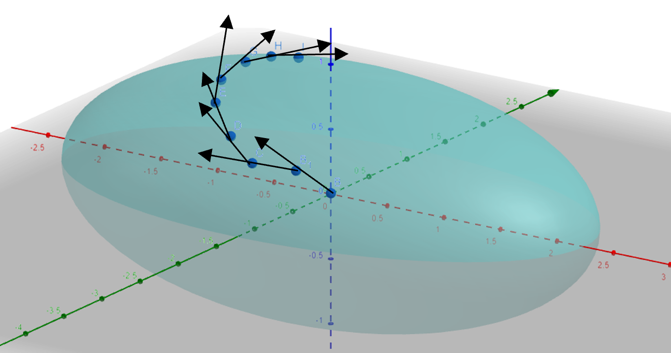
In addition, a conceptual visualization of the Algorithm 1 in $3D$ space is shown in Fig. 1. In this space, the constraint in (19) could be seen as an ellipsoid. The algorithm searches for a direction that increases the effectiveness $\alpha$ at each iterative step. Furthermore, the update law for step size $\lambda$ in (26) ensures that the algorithm eventually terminates on the boundary at time step $M$, as proved in (29).

In this section, we validate the efficacy of the MH-FDIA using two case studies: a simulation of a linear regulation control system of the IEEE 14-bus network, and an experiment of a nonlinear path-following control system of a wheeled mobile robot (WMR). Firstly, we validate the theoretical performance of the MH-FDIA and analyze the influence of the parameters of Algorithm 1 on the MH-FDIA’s performance using the linear bus system simulation. Through the nonlinear WMR experiment, we showcase the implementation of the proposed MH-FDIA on a nonlinear system and demonstrate its seamless performance in real-world scenarios.

References

- [1] B. Brentan, P. Rezende, D. Barros, G. Meirelles, E. Luvizotto, J. Izquierdo, Cyber-attack detection in water distribution systems based on blind sources separation technique, Water 13 (6) (2021) 795.
- [2] G. Liang, S. R. Weller, J. Zhao, F. Luo, Z. Y. Dong, The 2015 ukraine blackout: Implications for false data injection attacks, IEEE Transactions on Power Systems 32 (4) (2017).
- [3] J. R. Reeder, C. T. Hall, Cybersecurity’s pearl harbor moment: Lessons learned from the colonial pipeline ransomware attack (2021).
- [4] W. Xu, K. Ma, W. Trappe, Y. Zhang, Jamming sensor networks: attack and defense strategies, IEEE network 20 (3) (2006) 41–47.
- [5] F. Pasqualetti, F. Dörfler, F. Bullo, Attack detection and identification in cyber-physical systems, IEEE transactions on automatic control 58 (11) (2013) 2715–2729.
- [6] L. Hu, Z. Wang, Q.-L. Han, X. Liu, State estimation under false data injection attacks: Security analysis and system protection, Automatica 87 (2018) 176–183.
- [7] T.-Y. Zhang, D. Ye, False data injection attacks with complete stealthiness in cyber–physical systems: A self-generated approach, Automatica 120 (2020) 109117.
- [8] Y. Liu, P. Ning, M. K. Reiter, False data injection attacks against state estimation in electric power grids, ACM Transactions on Information and System Security 14 (1) (2011) 1–33.
- [9] Y. Mo, B. Sinopoli, False data injection attacks in control systems, in: Preprints of the 1st workshop on Secure Control Systems, 2010, pp. 1–6.
- [10] X. Liu, Z. Bao, D. Lu, Z. Li, Modeling of local false data injection attacks with reduced network information, IEEE Transactions on Smart Grid 6 (4) (2015) 1686–1696.
- [11] A.-Y. Lu, G.-H. Yang, False data injection attacks against state estimation without knowledge of estimators, IEEE Transactions on Automatic Control (2022).
- [12] M. Mohammadpourfard, F. Ghanaatpishe, M. Mohammadi, S. Lakshminarayana, M. Pechenizkiy, Generation of false data injection attacks using conditional generative adversarial networks, in: 2020 IEEE PES Innovative Smart Grid Technologies Europe (ISGT-Europe), IEEE, 2020, pp. 41–45.
- [13] Y. Zheng, A. Sayghe, O. Anubi, Algorithm design for resilient cyber-physical systems using an automated attack generative model, TechRxiv (2021).
- [14] A. Khazraei, S. Hallyburton, Q. Gao, Y. Wang, M. Pajic, Learning-based vulnerability analysis of cyber-physical systems, in: 2022 ACM/IEEE 13th International Conference on Cyber-Physical Systems (ICCPS), IEEE, 2022, pp. 259–269.
- [15] T. Sui, Y. Mo, D. Marelli, X. Sun, M. Fu, The vulnerability of cyber-physical system under stealthy attacks, IEEE Transactions on Automatic Control 66 (2) (2020) 637–650.
- [16] J. B. Rawlings, D. Q. Mayne, M. Diehl, Model predictive control: theory, computation, and design, Vol. 2, Nob Hill Publishing Madison, WI, 2017.
- [17] L. Zou, Z. Wang, J. Hu, Q.-L. Han, Moving horizon estimation meets multi-sensor information fusion: Development, opportunities and challenges, Information Fusion 60 (2020) 1–10.
- [18] J. Löfberg, Oops! i cannot do it again: Testing for recursive feasibility in mpc, Automatica 48 (3) (2012) 550–555.
- [19] K. R. Muske, J. B. Rawlings, J. H. Lee, Receding horizon recursive state estimation, in: American Control Conference, IEEE, 1993, pp. 900–904.
- [20] S. Weerakkody, O. Ozel, Y. Mo, B. Sinopoli, et al., Resilient control in cyber-physical systems: Countering uncertainty, constraints, and adversarial behavior, Foundations and Trends® in Systems and Control 7 (1-2) (2019) 1–252.
- [21] C. V. Rao, J. B. Rawlings, D. Q. Mayne, Constrained state estimation for nonlinear discrete-time systems: Stability and moving horizon approximations, IEEE transactions on automatic control 48 (2) (2003) 246–258.
- [22] D. A. Allan, J. B. Rawlings, Moving horizon estimation, in: Handbook of Model Predictive Control, Springer, 2019, pp. 99–124.
- [23] O. Kosut, L. Jia, R. J. Thomas, L. Tong, Limiting false data attacks on power system state estimation, in: 44th Annual Conference on Information Sciences and Systems, IEEE, 2010.
- [24] Y. Zheng, O. M. Anubi, Attack-resilient weighted l1 observer with prior pruning, in: American Control Conference, 2021, pp. 340–345.
- [25] A. Khazraei, S. Hallyburton, Q. Gao, Y. Wang, M. Pajic, Learning-based vulnerability analysis of cyber-physical systems, arXiv preprint arXiv:2103.06271 (2021).
- [26] E. Scholtz, Observer-based monitors and distributed wave controllers for electromechanical disturbances in power systems, Ph.D. thesis, Massachusetts Institute of Technology (2004).
- [27] D. Xie, S. Wang, Y. Wang, Trajectory tracking control of differential drive mobile robot based on improved kinematics controller algorithm, in: 2018 Chinese Automation Congress (CAC), IEEE, 2018, pp. 2675–2680.
- [28] Y. Zheng, O. M. Anubi, Attack-resilient observer pruning for path-tracking control of wheeled mobile robot, in: Dynamic Systems and Control Conference, Vol. 84287, American Society of Mechanical Engineers, 2020, p. V002T33A001.
- [29] S. J. Julier, J. K. Uhlmann, New extension of the kalman filter to nonlinear systems, in: Signal processing, sensor fusion, and target recognition VI, Vol. 3068, International Society for Optics and Photonics, 1997, pp. 182–193.