Stability of quantised vortices in two-component condensates

The equations of motion of a trapped two-dimensional two-component condensate are,

where $\Psi_{j}$ are the macroscopic wavefunctions for the components $j=1,2$, ${\tilde{\mu}_{j}}$ are the chemical potentials, ${\hat{K}}_{j}=-\frac{\hbar^{2}}{2M_{j}}\nabla^{2}$ are the kinetic energy operators, $G_{j}$ are the 2D self-interaction parameters and $G_{12}$ is the 2D inter-species interaction parameter. The 2D trapping potential $V(\mathbf{x})$ (where $\mathbf{x}=(x,y)$) is taken to be a cylindrical box-trap of radius $r_{B}$ and height $V_{0}$. It is convenient to assume the circularly symmetric form,

where $r^{2}=x^{2}+y^{2}$. Assuming that $V_{0}$ is larger than both chemical potentials, the two species are essentially confined in the region $r<r_{B}$; within this region, $V(r)$ is negligible. The quantity $a$ is a smoothing parameter. We assume the system is sufficiently low temperature that thermal noise and dissipation can be neglected. The assumption of an effectively two-dimensional system can be satisfied in practice by imposing a strong confinement of both components in the vertical direction, e.g. a harmonic potential with frequency $\omega_{z}\gg\tilde{\mu}_{j}/\hbar$, such that the dynamics in the extra dimension are frozen out (see Appendix A).

The system of equations (3) can be derived from the following action,

where the free energy density for each component $j$ and inter-species interaction energy density are respectively defined as,

Since independent phase rotations of $\Psi_{1}$ and $\Psi_{2}$ are symmetries of $\mathcal{S}$, we obtain two conserved currents

where $n_{j}=|\Psi_{j}|^{2}$ is the number density of component $j$ and $\mathbf{v}_{j}=\frac{\hbar}{M_{j}}\bm{\nabla}\mathrm{arg}(\Psi_{j})$ is its velocity. In a closed system, one can integrate over space to find that the number of atoms in each species, $N_{j}=\int n_{j}d^{2}\mathbf{x}$, is conserved by the evolution dictated by (3). Hereafter, we fix the number of atoms in the first component $N_{1}$ and treat $\eta=N_{2}/N_{1}$ as our variable.

An approximate expression for the ground state solution of equations (3) is provided by the Thomas-Fermi approximation: neglecting the kinetic energy terms, within the trap (where $V(r)\simeq 0$) the steady state solutions of (3) satisfy,

Since the two components are immiscible for $G_{12}>\sqrt{G_{1}G_{2}}$ Timmermans 1998, we can assume that component 2 is confined to the region $A_{2}=\pi r_{0}^{2}$ and component 1 occupies the remaining space $A_{1}=\pi(r_{B}^{2}-r_{0}^{2})$. We then have $n_{1}=N_{1}/A_{1}$ and $n_{2}=N_{2}/A_{2}$ so that the chemical potentials are approximately,

In this work, we consider systems with a vortex in $\Psi_{1}$ and no vortex in $\Psi_{2}$. In the stationary state, solutions of (3) are of the form,

where $\ell$ is the winding number of the vortex. The corresponding velocity field is $\mathbf{v}_{1}=\frac{\hbar\ell}{M_{1}r}\hat{\mathbf{e}}_{\theta}$ where $\hat{\mathbf{e}}_{\theta}$ is the unit vector in the azimuthal direction. We focus on the case $\ell=2$, however, we expect our conclusions to extend to vortices of higher winding numbers.

In the rest of the paper we express the governing equations (3) in dimensionless form using the following characteristic units of length, time and density,

where $\tilde{\mu}_{1,0}=\tilde{\mu}_{1}(\eta=0)$ is the chemical potential of species 1 in the vortex state when species 2 is absent In other words, we perform the following rescalings,

so that (3) becomes,

where we have defined the new dimensionless parameters,

Note the true total number of atoms can be recovered from $N_{j}=\int d^{3}\mathbf{x}|\Psi_{j}|^{2}$ in these units by multiplying by a factor of $\hbar^{2}/M_{1}G_{1}=d_{1}/\sqrt{8\pi}a_{1}$, where $d_{1}$ is the width of species 1 in the vertical direction and $a_{1}$ is its scattering length (see Appendix A).

Since $\xi_{1}\ell$ (where $\xi_{1}$ is the healing length of the condensate 1 for $\eta=0$) is the characteristic core size of an $\ell$-vortex, in the new units the vortex core now has radius $\sim\ell$. Furthermore, since the density of condensate 1 approaches $n_{0}$ far from the vortex axis where $n_{2}\to 0$, in the new units the bulk value of $n_{1}$ will approach $\mu_{1}$.

In these units, the problem depends only on $m_{2}$, $g_{2}$, $g_{12}$, the parameters in the trapping potential and the chemical potentials $\mu_{j}$. The latter are related to the total number of atoms in the ground state (see next section). The s–wave scattering lengths for the ⁸⁷Rb and ¹³³Cs mixture Pattinson et al. 2013 are $a_{1}=100a_{0}$, $a_{2}=280a_{0}$ and $a_{12}=650a_{0}$ [26] where $a_{0}$ is Bohr radius and hereafter the subscripts $1$ and $2$ refer respectively to the ⁸⁷Rb and ¹³³Cs components. In Appendix A, we show that when both species are subject to the same strong vertical confinement, the dimensionless interaction parameters are $g_{2}=2.04$ and $g_{12}=5.65$. The mass ratio is simply $m_{2}=133/87$. For the trapping potential, we fix $a=5$ and $V_{0}=5$ so that there is essentially a hard wall located at $r=r_{B}$. For the trap radius, we pick $r_{B}=40$ so that the trap is not too small to prohibit the instabilities under consideration but not so large that the problem becomes computationally impractical.

To solve for the stationary profiles $n_{1,2}$, we evolve (13) in imaginary time $\tau=it$. This amounts to making the replacement $i\partial_{t}\to-\partial_{\tau}$ in (3). Starting from a sensible initial condition, the population of the higher energy modes will then decrease exponentially with increasing $\tau$, leaving essentially only the ground state at late times. Since the anticipated densities are independent of the azimuthal coordinates, the speed of the computation is increased by working in polar coordinates. We therefore solve the following coupled set of equations,

where $\nabla_{r}^{2}=\partial_{r}^{2}+\frac{1}{r}\partial_{r}$ and $Y_{j}=|\Psi_{j}|=\sqrt{n_{j}}$. We work on a radial grid $r=[\Delta r,r_{B}+5]$ with $\Delta r=0.05625$ such that are $800$ radial points and use an imaginary time step $\Delta\tau=4\times 10^{-4}$. The evolution is performed using a $4^{\mathrm{th}}$ order Runge-Kutta algorithm with the radial derivatives approximated using finite difference stencils.

The first step is to fix a value for $N_{1}$ against which we can compare the effect of increasing $\eta$. This value is determined by solving (15) for $\eta=0$, using the fact that $\mu_{1}(\eta=0)=1$, and integrating over the resulting profile to get $N_{1}=\int d^{2}\mathbf{x}n_{1}(\eta=0)$. For $r_{B}=40$ and $\ell=2$, we have $N_{1}\simeq 4824$. Again, since this is the atom number in dimensionless variables, one must multiply by the dimensionless ratio $d_{1}/\sqrt{8\pi}a_{1}$ to find the true total number of atoms.

The second step is to choose an initial condition when the second component is added. We start by considering case the where no vortex is present ($\ell=0$) with component 2 localised in the centre of the system and component 1 surrounding it. A subtlety of the problem is that if we want to keep $N_{1,2}$ fixed, the chemical potentials must vary to accommodate these constraints. A priori, we do not know the values of $\mu_{1,2}$ and must determine them during the imaginary time evolution. We start by guessing their values using the Thomas-Fermi approximation (9), which in dimensionless units gives $\mu_{1}=N_{1}/\pi(r_{B}^{2}-r_{0}^{2})$ and $\mu_{2}=\eta g_{2}N_{1}/\pi r_{0}^{2}$. Since we consider $\eta$ to be very small, we take 1 as our initial guess for the value of $\mu_{1}$ and invert the first relation to find the value of $r_{0}$. The second relation provides a guess for $\mu_{2}$. The densities are then $n_{1}(r_{0}<r<r_{B})=\mu_{1}$ and $n_{2}(r>r_{0})=\mu_{2}/g_{2}$. We evolve these profiles forward in imaginary time, renormalising $\Psi_{1,2}$ after each time step to keep the values of $N_{1,2}$ fixed. After a long time, the system will have relaxed to its lowest energy state, however, there will be residual time dependence due to the fact that the chemical potentials were chosen incorrectly. We can use this time dependence to infer the shift in $\mu_{j}$ using $Y_{j}(\tau+\Delta\tau)=e^{-\delta\mu_{j}\Delta\tau}Y_{j}(\tau)$, so that the true chemical potentials are $\mu_{1}=1+\delta\mu_{1}$ and $\mu_{2}=\eta g_{2}N_{1}/\pi r_{0}^{2}+\delta\mu_{2}$ respectively. The evolution is terminated once the changes $\delta\mu_{1}$ and $\delta\mu_{2}$ over a time step are both less than $10^{-6}$. This is suitably small given that $\mu_{j}\sim\mathcal{O}(1)$ for both species and is computationally feasible when solving for a large range of $\eta$ values.

In the third step, we imprint a vortex by setting $\ell\neq 0$ in (15), taking the ground states obtained from step 2 as the initial condition. We evolve again in imaginary time (using the same termination criterion) to find the stationary vortex solutions and update the chemical potentials accordingly.

In Fig. 1, we present the resulting density profiles $n_{1,2}$ as a function of $r$ for a vortex with $\ell=2$. We see that component 2 stays inside the core of the vortex in component 1, and its effect is to widen the core. It is remarkable that even the small values of $\eta$ which we consider here have such a significant effect. This widening becomes more significant as $\eta$ increases. We also display the variation of the chemical potentials with $\eta$ in the inset of the right panel. $\mu_{1}$ increases with $\eta$ by a very small amount due to the repulsive effect of species 2 inside the vortex core. This forces more of the $N_{1}$ particles into the bulk of the condensate, increasing the mean value of the density in this region. $\mu_{2}$ increases much more obviously with $\eta$ since $N_{2}$ is increasing and therefore the density of species 2 must go up accordingly. Note however that $\mu_{2}$ does not vanish as $\eta\to 0$. This is because there is a contribution of the curvature of $n_{2}$ to the chemical potential. Indeed, solving the equation in (15) for $Y_{2}$ in limit $r\to 0$ gives the relation $\mu_{2}=(g_{2}n_{2}-n_{2}^{\prime\prime}/2m_{2}n_{2})|_{r=0}$. This does not go to zero as $n_{2}\to 0$ since the ratio $n_{2}^{\prime\prime}/n_{2}$ stays finite in this limit.

Let $\delta\psi_{j}$ be small fluctuations about $\Psi_{j}$ and write the following Ansatz,

with $u_{j}$ and $v_{j}$ functions of $r,t$ and $m$, where $m$ is the azimuthal wavenumber. When the equations of motion (13) are linearized, since neither $n_{1,2}$ nor $\mathbf{v}_{1,2}$ depend on $\theta$, each $m$ component evolves independently of the others. Due to the symmetries $u_{j}^{*}(m)=v_{j}(-m)$ and $v_{j}^{*}(m)=u_{j}(-m)$, we can restrict our attention to $m\geq 0$ modes without loss of generality. The fluctuations $|U\rangle=(u_{1},u_{2},v_{1},v_{2})^{\mathrm{T}}$ obey the following coupled set of equations,

The operator $\widehat{L}$ is,

where,

and the coupling between fluctuations of both species is determined by $\varepsilon=g_{12}\sqrt{n_{1}n_{2}}$. Note that for immiscible fluids, the region of overlap of the two components is small. $\varepsilon$ will be small in this region and zero everywhere else. The fields $u_{j}$ and $v_{j}$ are related to the components of the density field by,

The equations in (17) can be derived from the action $S_{\mathrm{BdG}}=\int dtd^{2}\mathbf{x}\mathcal{L}_{\mathrm{BdG}}$ where,

$S_{\mathrm{BdG}}$ is invariant when each of the fields $u_{j}$ and $v_{j}$ simultaneously undergo the same phase rotation. The corresponding conserved quantity is the Bogoliubov norm,

where $\gamma^{0}=\mathrm{diag}(1,1,-1,-1)$ is the zeroth gamma matrix. Notice that due to the presence of the cross-terms with coefficient $\varepsilon$ in (21), excitations of species 1 can be converted into excitations of species 2 and vice versa. However, the total number of excitations, as measured by $\mathcal{N}_{\mathrm{BdG}}$, is conserved.

Since the background is stationary, we can further decompose the fluctuations into the separate frequency components,

where $a_{\omega}$ and $|\widetilde{U}\rangle$ respectively satisfy,

The first equation is solved by $a_{\omega}\propto e^{-i\omega t}$ up to an arbitrary constant, whilst the second must be solved numerically. The Hamiltonian for stationary modes is related to the Bogoliubov norm via $H_{\mathrm{BdG}}=\int d^{2}\mathbf{x}\mathcal{H}_{\mathrm{BdG}}=\omega\mathcal{N}_{\mathrm{BdG}}$. Therefore a positive frequency mode with negative norm (or a negative frequency mode with positive norm) has negative energy. The sign of the energy plays an important role in the discussion of the instability.

To solve the second equation in (24) computationally, we write the radial derivative terms using finite difference stencils on a discrete $r$-grid then find the eigenvalues and eigenfunctions of the resulting matrix $\widehat{L}$. The eigenfunctions are normalised so that $|\mathrm{Re}[\mathcal{N}_{\mathrm{BdG}}]|=1$, which gives an unambiguous normalisation condition for all solutions obtained. We place a Dirichlet boundary condition at large $r$, although this does not play a significant role as it is applied in a region where $V(r)$ is large, hence, modes with energy lower than the barrier height quickly decay to zero inside this region. A discussion of the boundary conditions at $r=0$ can be found in Appendix B.

In Fig. 2, we present the eigenvalues $\omega$ as a function of $\eta$ for $\ell=2$ and $r_{B}=40$. There are two distinct types of excitation. Bulk excitations (shown in black) predominantly occupy the region outside of the vortex core and are associated with collective excitations of the condensate, or phonons at low wavenumbers. Indeed, on panel (c), it can be seen that these modes have a large oscillatory component in the large $r$ region. They have positive energy ($H_{\mathrm{BdG}}>0$) and are largely unaffected by increasing $\eta$, which influences only the vortex core. There is a second class of excitation which we refer to as vortex modes. These have negative energy ($H_{\mathrm{BdG}}<0$) at low $\eta$ and are mainly localised around the vortex axis, as illustrated in panel (c). In panel (a), we see that there is only one such mode for the $\ell=2$ vortex represented by the red line. Since this mode occupies the same region as component 2, it is strongly affected when $\eta$ is increased. Indeed, the frequency of the vortex mode on panel (a) can be seen to decrease rapidly even for relatively small amounts of component 2. In the presence of a dissipation mechanism, these modes will be excited since they lower the total energy of the system, i.e. they are an energetic instability.

When $\mathrm{Re}[\omega]$ of the vortex mode crosses that of a bulk excitation, the two couple to produce a complex conjugate pair of modes with vanishing Bogoliubov norm. This leads to the appearance of isolated bubbles in $\mathrm{Im}[\omega]$ in panel (b). The mode with $\mathrm{Im}[\omega]>0$ represents a dynamical instability, that is, the central vortex spontaneously sheds its energy into a sound wave in the bulk even without a dissipation mechanism. This does not violate energy conservation since the total energy of the mode encoding this behaviour is zero ($H_{\mathrm{BdG}}=0$). The complex conjugate mode describes the time reversed process, i.e. absorption of a sound wave by the central vortex. In panel (d), we show how the waveforms of the two modes in panel (c) combine to produce the real and imaginary parts of the instability.

Note that for large enough $r_{B}$ (larger than considered here) i.e. in the limit that finite size effects become negligible, the bubbles in $\mathrm{Im}[\omega]$ eventually merge into a continuum Giacomelli and Carusotto 2020. In that case, there is a dynamical instability at $\eta=0$ for all larger trap sizes and, in particular, in the infinite system limit.

We also show in Fig. 3 the effect of increasing $\eta$ on the waveform of the vortex mode around the vortex axis. The main feature is that the amplitude of the mode at $r=0$ is suppressed as the number of atoms in species 2 is increased. This will be addressed in the next section.

For large $\eta$, the vortex mode has a frequency lower than all positive frequency bulk excitations. At a critical $\eta$ value, which we call $\eta_{c}$ (the black dot in Fig. 2(a)), the frequency of the vortex mode changes sign. Since the Bogoliubov norm of this mode is negative, the energy of the vortex mode is positive for $\eta>\eta_{c}$ and it will no longer get excited when a dissipation mechanism is included. Furthermore, since the negative frequency bulk excitations have negative norm, they have positive energy and the vortex mode cannot mix with these modes to produce a dynamical instability with zero energy. Above $\eta_{c}$, the system is stabilised by the presence of the second component. The next section will explore the mechanism underpinning this stabilisation whilst Section IV will demonstrate stability via a full numerical simulation of (13).

From Fig. 2(a), we find the value $\eta_{c}=5.933\times 10^{-4}$. Since the value obtained will in general depend on the resolution used in the numerics, we estimate that the infinite resolution limit would yield the value $\eta_{c}=5.936\times 10^{-4}$ (details in Appendix C). Note that this value is also specific to an $\ell=2$ vortex in a trap of a radius $r_{B}=40$ and will in general depend on both these parameters. Due to computational cost, we do not study this dependence here.

A computation of the mode energy in (21) gives insight into the behaviour around $\eta_{c}$. In Fig. 4, we integrate the (vortex mode) energy density components in (21) over space and plot as a function of $\eta$. The total energy $H_{\mathrm{BdG}}$ is negative at low $\eta$ except inside finite windows where it is vanishing due to the dynamical instability. At the edge of these windows, the amplitudes of the normalised mode diverges, as reflected in the components of $H_{\mathrm{BdG}}$, but does so in a way that keeps the total energy finite. The energy of species 2 fluctuations $H_{\mathrm{BdG},2}$ is always positive whilst the interaction energy $H_{\mathrm{BdG,int}}$ between fluctuations of each species is always negative. The energy of species 1 fluctuations $H_{\mathrm{BdG},1}$ is initially negative but becomes positive around $\eta=2.33\times 10^{-4}$. Correspondingly, the maximum amplitude of the vortex mode waveform shifts outwards into a region where it has positive energy density (see Fig. 3). Since $H_{\mathrm{BdG,int}}$ is close to the value of $-2H_{\mathrm{BdG},2}$ the total mode energy is still negative even when $H_{\mathrm{BdG},1}=0$. Interestingly, in this regime, the energetic instability of the vortex mode is a result of the interaction between fluctuations of the two species, rather than being an inherent property of the vortex in species 1 alone. Increasing $\eta$ further, the total energy changes sign at $\eta_{c}$. This coincides with $H_{\mathrm{BdG},1}$ exceeding the value of $H_{\mathrm{BdG},2}$.

To interpret why the vortex mode is shifted to lower frequency with increasing $\eta$, we apply a WKB method. This method has been demonstrated to give insight into the physical origin of vortex instabilities Patrick et al. 2022a as well as providing reasonable estimates of the unstable mode frequencies Patrick et al. 2022b. Following the procedure outlined in Patrick et al. 2022b, we first write a WKB Ansatz,

where $p$ is the local component of the wavevector in the radial direction and we assume $|p^{2}|\gg|\partial_{r}p|$, $|p\mathcal{A}_{j}|\gg|\partial_{r}\mathcal{A}_{j}|$ and similarly for $\mathcal{B}_{j}$. Taking only the leading order contributions and eliminating the four amplitudes, (24) becomes,

where,

and $\Omega=\omega-m\ell/r^{2}$ is the frequency in the frame rotating with the vortex. We have also defined a pair of effective wavevectors by,

where the effective azimuthal numbers are,

Hence, we can identify the condition in (26) as two coupled dispersion relations respectively describing excitations of components 1 and 2 interacting through a small overlap region where $\varepsilon$ is non-zero. As a first approximation, we study the non-interacting case with $\varepsilon\to 0$. We are particularly interested in the fluctuations of component 1 (since this is where the instability arises) which approximately satisfy $\mathcal{D}_{1}(k_{1})\simeq 0$. This condition has two sets of solutions for $p$ which are decoupled from each other. The first type are evanescent over the whole system whereas the second can propagate. We are only interested in the second type. These are determined by,

Points where $p=0$ correspond to turning points, i.e. radial locations where an incoming wave instantaneously comes to rest before reversing its direction and propagating back out Patrick et al. 2022b. We can therefore view $W_{+}$ as an effective potential; when $W_{+}<0$ these waves are propagating whilst for $W_{+}>0$ they are evanescent.

To see the effect of adding a second component, one can expand the $\widetilde{m}_{1}^{2}$ term in $W_{+}$:

In the absence of the second component, this potential has a cavity located about $r=0$ where waves with correct frequency can become trapped as bound states These states approximately satisfy $\cos I\simeq 0$ Patrick et al. 2022b, where $I=\int_{{}_{\mathrm{cav}}}\!p\,dr$ is the phase integral inside the cavity in the vortex core (see Appendix D for a further discussion). When a second species is present inside the vortex core, the final term in (31) creates a bulge in the potential around $r=0$ (as shown in Fig. 5) thereby decreasing the amount of space the mode has to fit in the cavity. This bulge inhibits wave propagation in the immediate vicinity of the vortex axis, explaining the feature of Fig. 3 where the amplitude of the waveform drops on the vortex axis with increasing $\eta$. Conventional wisdom gained from the 1D Schrödinger equation in quantum mechanics would dictate that this should raise the frequency of the bound state, however, this is not the case here as we now illustrate.

To solve the resonance condition in the cavity, one should compute $I(\omega)$ for all frequencies which probe the cavity before finding the one which solves $\cos I=0$. For small $\eta$, we show in Appendix D that the integral near the bottom of the cavity (for $m=\ell=2$) can be expanded as,

where $\omega_{0}$ is the maximum frequency which probes the cavity and $n^{\prime\prime}_{2,0}$ is the curvature of the density of component 2 on the axis. This expression demonstrates that $I$ decreases as $\omega$ increases, i.e. $\partial_{\omega}I<0$. More generally, the reason for this difference with the standard Schrödinger picture (in which $\partial_{\omega}I>0$) is that the vortex mode in the WKB picture is on the lower branch of the dispersion relation where $\Omega<0$ (which is related to the negative norm of the mode). On this branch, the root with $p>0$ has negative group velocity $\partial_{p}\omega<0$, i.e. decreasing $\omega$ increases the value of $p$. Therefore, since increasing $\eta$ will decrease $p$ through the final term in (31), the frequency of the bound state decreases to keep $I$ fixed at the value satisfying the resonance condition.

Although the WKB method correctly predicts the decrease of the vortex mode frequency with increasing $\omega$, it fails at providing the quantitative value. This is to be expected since the approximation works best for high frequencies in regions where the background functions change gradually. Indeed, in Patrick et al. 2022b, the WKB estimates are practically indistinguishable from numerical calculations for bulk excitations, whilst for the vortex mode (which occupies a region where the background density quickly changes) the WKB estimate differs notably from the numerics. When $\eta\neq 0$, the frequency is lower than the $\eta=0$ case and the bulge in $W_{+}$ makes background variations more significant. Both of these features decrease the quantitative power of the WKB approximation.

We first evolve (3) for $\eta=0$, i.e. when the second species is absent. For our spatial grid, we take $x\in[-(r_{B}+5),r_{B}+5]$ and similarly for $y$ with $N=512$ spatial points. We take $\Delta t=5\times 10^{-3}$ and evolve using a split-step Fourier method for $2\times 10^{5}$ steps in time, saving every $200^{\mathrm{th}}$ frame. For the initial condition, we seed the stationary vortex profile for $\ell=2$ and $r_{B}=40$ with the unstable mode of amplitude $|a_{\omega}(t=0)|=10^{-3}$. We note that the corresponding resolution in the radial direction is $256$ points, which differs from the value of $800$ used in Section II.4. The reduced resolution slightly shifts the location of the instability bubbles in Fig. 2. Hence, for consistency, we repeat the procedure in Section II.4 and III.1 for $\Delta\tau=5\times 10^{-3}$ and 256 radial grid points when producing the initial condition, since we want to precisely seed the mode which is unstable in our non-linear simulations. A comparison of the normal mode spectra at different resolutions can be found in Appendix C.

The results are shown in Fig. 6. Panels (a-c) show the density at early, intermediate and late times, with constant density contour superimposed in red/white, and panels (d-f) show the phase at the same times. In panels (a) and (d), the vortex is close to its stationary profile whilst in panels (b) and (e), a deformation of the central vortex can be seen. In panels (c) and (f), the central vortex has split into two $\ell=1$ vortices. The density contours indicate that this splitting is accompanied by the production of a bulk excitation, namely, a sound wave with $m=2$. At sufficiently late times, the vortices move back into the centre due to finite system effects studied in Patrick et al. 2022a. Since our focus is on the splitting mechanism, we do not discuss this behaviour further here. In the presence of dissipation, the initial splitting described here continues and the vortices separate widely, as we show in Section IV.4.

In panel (g), we perform a Fourier decomposition of the density $n=(2\pi)^{-1}\int d\theta e^{im\theta}n_{m}$ and display modulus of the Fourier components $m=0,2$ at the location $r=1.37$. This location corresponds to the peak of the radial waveform $n_{m=2}(r)$. At first, the $m=2$ mode grows exponentially in line with the prediction of Fig. 2. Around $t=800$, the $m=2$ mode reaches a maximum amplitude and starts to decay as the vortices move back into the centre. Near the maximum amplitude of $n_{m=2}$, we also observe the non-linear effect of the unstable mode on the $m=0$ component. This is simply the backreaction of the growing mode onto the background density profile, which can be physically understood as the condensate filling in the centre as the vortices move apart.

The instability is associated with a decrease of incompressible (vortex) energy and an increase in compressible (sound wave) energy. The energy of the system can be decomposed as,

where the kinetic energy $E_{\mathrm{kin}}$ is associated with a non-vanishing velocity field and the quantum energy $E_{q}$ results from density variations. $\mathcal{E}_{\mathrm{pot}}=Vn$ and $\mathcal{E}_{\mathrm{int}}=n^{2}/2$ are the usual potential and interactions energy densities respectively. The kinetic energy can be further split into compressible and incompressible parts by defining $\mathbf{u}=\sqrt{n}\bm{\nabla}\Phi$ and writing $\mathbf{u}=\mathbf{u}_{c}+\mathbf{u}_{i}$, where the incompressible part obeys $\bm{\nabla}\cdot\mathbf{u}_{i}=0$. Operationally, the compressible part can be found by performing a Fourier transform $\mathcal{F}$, projecting $\mathbf{u}$ onto the wavevector $\mathbf{k}$ and computing the inverse Fourier transform $\mathcal{F}^{-1}$. That is, $\mathbf{u}_{c}=\mathcal{F}^{-1}[\mathbf{k}(\mathbf{k}\cdot\mathcal{F}\mathbf{u})/||\mathbf{k}||^{2}]$ and $\mathbf{u}_{i}=\mathbf{u}-\mathbf{u}_{c}$. Since $\mathbf{u}_{c}$ and $\mathbf{u}_{i}$ have zero overlap, the kinetic energy can be written $E_{\mathrm{kin}}=E_{c}+E_{i}$, with $E_{c}=\int d^{2}\mathbf{x}\,\mathbf{u}_{c}$ and similarly for $E_{i}$. We display $E_{q}$, $E_{i}$ and $E_{c}$ in panels (h), (i) and (j) respectively. The incompressible energy decreases as the vortices move apart (into a lower energy configuration) and the compressible and quantum energies increase in response. The two vertical black lines in the rightmost panels correspond to the times in panels (b) and (c) respectively.

To assess the effect of adding a small amount of component 2 inside the vortex core of component 1, we repeat the simulation of the last section for various values of $\eta$. In particular, we start from the stationary profiles for condensate 1 and 2 and perturb the system by inserting the unstable mode with an amplitude $10^{-3}$. The values of $\eta$ chosen correspond to the peaks of $\mathrm{Im}[\omega]$ in the stability windows at the chosen resolution.

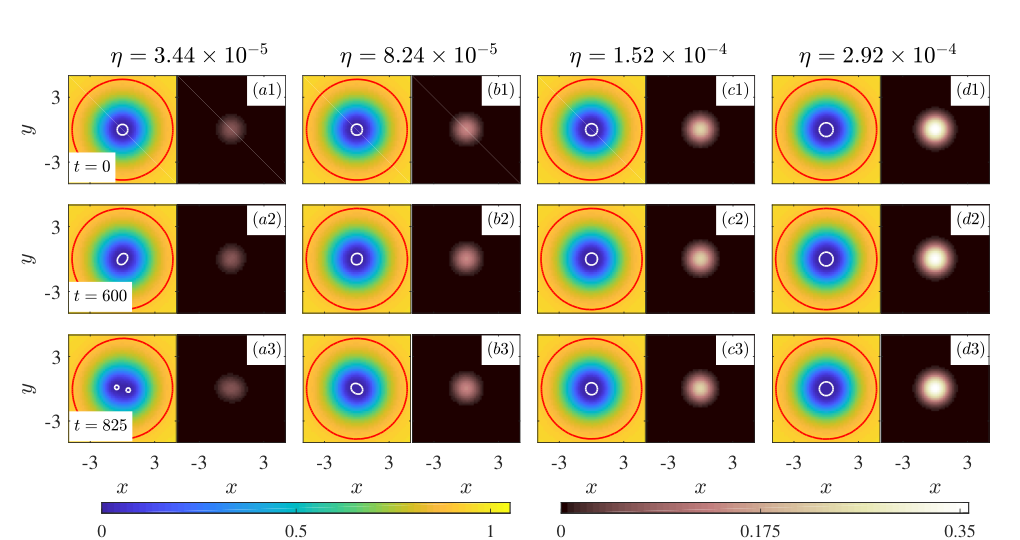
In Fig. 7, we display the densities of species 1 and species 2 for four values of $\eta$ at the same times depicted as the $\eta=0$ case in Fig. 1. As $\eta$ increases, we clearly see that the vortices have separated less at a given instant of time when compared with the single component system, thereby demonstrating the stabilising effect of the second species. Since the minute separation becomes less and less transparent from the density plots with increasing $\eta$, we show on Fig. 8 the growth of the $m=2$ mode in the vortex core. Here, we clearly see that both the oscillation frequency and growth rate decrease with increasing $\eta$. The values of $\mathrm{Re}[\omega]$ and $\mathrm{Im}[\omega]$ correspond to those predicted by the linear analysis in Fig. 2 (see Appendix C for an explicit comparison).

In general, the unstable mode in the spectrum of the MQV is associated with its splitting into a cluster of SQVs, whose distribution is determined by the $m$-fold symmetry of the unstable mode. In single component systems, the cluster rotates in the direction of the net winding of the system, since each vortex essentially moves under the collective influence of all the others. The story is not so simple when a second component is added. The orbital frequency of the resulting cluster is given by $\mathrm{Re}[\omega]/m$, with $\mathrm{Re}[\omega]$ the oscillation frequency of the unstable mode. Hence, the frequency inversion for $\eta>\eta_{c}$ seen in Fig. 2 is associated with the reversal of the cluster’s orbital motion. We demonstrate this now with a numerical simulation.

We choose a series of $\eta$ values where the vortex is dynamically stable. Note here that dynamical stability below $\eta_{c}$ results from finite size effects for certain ranges of $r_{B}$, whilst above $\eta_{c}$ it persists for all trap sizes, as shown by Fig. 2. Using the same resolution as the previous section, we now seed the stationary vortex profile with the vortex mode of amplitude $|a_{\omega}(t=0)|=2$. Due to the large amplitude, in all cases we observe a sudden burst of sound from the central vortex as the system relaxes through non-linear interactions. After this initial burst, we observe a stably orbiting vortex pair in the centre of the trap surrounded by small noise. On Fig. 9, we display snapshots of the density profiles of the two species at three different times. The red arrows indicate the direction of the orbital motion. For the two leftmost columns, the orbital motion is counter-clockwise, corresponding to $\mathrm{Re}[\omega]>0$ for the vortex mode below $\eta_{c}$. The atoms of species 2 are shared between the two $\ell=1$ vortices in the pair and track their motion. Conversely, the orbital motion is clockwise on the two rightmost columns, corresponding to $\mathrm{Re}[\omega]<0$ above $\eta_{c}$.

For large $\eta$ we find that a region of depleted density in component 1 persists between the two separated vortices and is occupied by component 2. We interpret this as the result of the waveforms in Fig. 3. For $\eta=0$, the maximum value of the waveform on the vortex axis non-linearly excites the $m=0$ mode as the vortices separate, causing atoms to fill in the space between them. For large $\eta$, the waveform decreases approaching $r=0$, suppressing the non-linear excitation of $m=0$ in that region. Physically, the presence of component 2 on the vortex axis prevents excitations in component 1 propagating there, which means there is nothing to increase the value of the density of component 1 at $r=0$ as the vortices separate.

In the presence of a dissipation mechanism, an MQV in a one-component condensate will still decay even if the vortex mode does not couple to any bulk excitations. The reason is that the vortex mode has negative energy, hence, its excitation lowers the total energy of the system, as required by the dissipation. The same is not necessarily true in a two-component system as we now show, since the vortex mode has a positive energy above $\eta_{c}$.

In Fig. 10, we present results of three simulations performed with damping. The initial conditions in panels (a), (b) and (c) are, respectively, the final frames of the simulations shown in Fig. 7(a), Fig. 9(a) and Fig. 9(d), corresponding to the same $\eta$ values indicated at the top of the figures. These respectively correspond to the lowest fraction of $\eta$ simulated which are unstable (panel (a)) and stable (panel (b)) when $\gamma_{1}=0$ and the largest $\eta$ value simulated above $\eta_{c}$ (panel (c)). As $\eta$ is small, damping applied to atoms of the second species will quickly reduce $N_{2}$ to zero. Hence, we only apply damping to the first component. This is achieved by replacing $i\partial_{t}$ by $(i-\gamma_{1})\partial_{t}$ in (13), taking the value $\gamma_{1}=5\times 10^{-2}$.

In Fig. 10(a1-3), the initial condition is a dynamically unstable vortex mode with low amplitude. In the three snapshots, we observe the central MQV splitting into a pair of SQVs rotating counter-clockwise with equal amounts of second component in the two cores. During the splitting, the second species remains confined to the vortex cores, rather than being dispersed across the system.

In panels (b1-3), the initial condition is two nearby SQVs surrounded by noise. The noise is quickly damped out and the vortices spiral out in the counter-clockwise sense with decreasing orbital frequency. In this regime, the vortices orbit in accordance with the regular point-vortex dynamics Barenghi and Parker 2016 which dictates the orbital frequency is approximately $\Omega=2/s^{2}$, where $s$ is the separation between vortices, with the atoms of species 2 playing a negligible role in the dynamics. In accordance with this expectation, the dynamics observed for $t>300$ at $\eta=3.4\times 10^{-5}$ (i.e. after the last frame shown on panel (a)) also follow the point-vortex behaviour. From this, we conclude that the modified dynamics in two component condensates is absent when species 2 atoms are split into distinct parcels which occupy the separate vortex cores. In other words, the stabilisation is a feature of a single parcel of species 2 atoms shared across the vortices.

To support this conclusion, in panels (c1-3), we take such a configuration as our initial condition. The corresponding vortex mode at this $\eta$ value has positive energy, hence, the separation of vortices (whilst retaining a single parcel of species 2 atoms) is associated with an energy gain relative to the stationary MQV. As the system evolves, the vortices orbit in the clockwise sense and damping reduces the vortex separation to lower the energy of the system. At late times, we recover a stationary, central MQV. This demonstrates that MQVs seeded with species 2 atoms above a critical fraction can be inherently stable objects even when a dissipation mechanism is present.

References

- Barenghi and Parker (2016) C. F. Barenghi and N. G. Parker, A primer on quantum fluids (Springer, 2016).
- Adhikari (2019) S. K. Adhikari, Laser Phys. Lett. 16, 085501 (2019).
- Adhikari and Muruganandam (2002) S. K. Adhikari and P. Muruganandam, Phys. Lett. A 301, 333 (2002).
- Srinivasan (2006) R. Srinivasan, Pramana 66, 3 (2006).
- Kuopanportti et al. (2015) P. Kuopanportti, N. V. Orlova, and M. V. Milošević, Phys. Rev. A 91, 043605 (2015).
- Pu et al. (1999) H. Pu, C. K. Law, J. H. Eberly, and N. P. Bigelow, Phys. Rev. A 59, 1533 (1999).
- Shin et al. (2004) Y. Shin, M. Saba, M. Vengalattore, T. A. Pasquini, C. Sanner, A. E. Leanhardt, M. Prentiss, D. E. Pritchard, and W. Ketterle, Phys. Rev. Lett. 93, 160406 (2004).
- Isoshima et al. (2007) T. Isoshima, M. Okano, H. Yasuda, K. Kasa, J. A. M. Huhtamäki, M. Kumakura, and Y. Takahashi, Phys. Rev. Lett. 99, 200403 (2007).
- Giacomelli and Carusotto (2020) L. Giacomelli and I. Carusotto, Phys. Rev. Research 2, 033139 (2020).
- Patrick et al. (2022a) S. Patrick, A. Geelmuyden, S. Erne, C. F. Barenghi, and S. Weinfurtner, Phys. Rev. Research 4, 043104 (2022a).
- Patrick et al. (2022b) S. Patrick, A. Geelmuyden, S. Erne, C. F. Barenghi, and S. Weinfurtner, Phys. Rev. Research 4, 033117 (2022b).
- Qin et al. (2016) J. Qin, G. Dong, and B. A. Malomed, Phys. Rev. A 94, 053611 (2016).
- Myatt et al. (1997) C. J. Myatt, E. A. Burt, R. W. Ghrist, E. A. Cornell, and C. E. Wieman, Phys. Rev. Lett. 78, 586 (1997).
- Hall et al. (1998) D. S. Hall, M. R. Matthews, J. R. Ensher, C. E. Wieman, and E. Cornell, Phys. Rev. Lett. 81, 1539 (1998).
- McCarron et al. (2011) D. J. McCarron, H. W. Cho, D. L. Jenkin, M. P. Köppinger, and S. L. Cornish, Phys. Rev. A 84, 011603 (2011).
- Papp et al. (2008) S. B. Papp, J. M. Pino, and C. E. Wieman, Phys. Rev. Lett. 101, 040402 (2008).
- Kronjäger et al. (2005) J. Kronjäger, C. Becker, M. Brinkmann, R. Walser, P. Navez, K. Bongs, and K. Sengstock, Phys. Rev. A 72, 063619 (2005).
- Tojo et al. (2010) S. Tojo, Y. Taguchi, Y. Masuyama, T. Hayashi, H. Saito, and T. Hirano, Phys. Rev. A 82, 033609 (2010).
- Kuopanportti et al. (2019) P. Kuopanportti, S. Bandyopadhyay, A. Roy, and D. Angom, Phys. Rev. A 100, 033615 (2019).
- Mason (2017) P. Mason, J. Phys. B: Atomic, Molecular and Optical Physics 50, 165002 (2017).
- Zhang et al. (2016) X. Zhang, L. Wen, C. Dai, R. Dong, H. Jiang, H. Chang, and S. Zhang, Sci. Rep. 6, 1 (2016).
- Dong et al. (2016) B. Dong, L. Wang, G. Chen, W. Han, S. Zhang, and X. Zhang, Ann. Phys. 373, 178 (2016).
- Ma et al. (2016) X. Ma, R. Driben, B. A. Malomed, T. Meier, and S. Schumacher, Sci. Rep. 6, 34847 (2016).
- Kawaguchi and Ohmi (2004) Y. Kawaguchi and T. Ohmi, Phys. Rev. A 70, 043610 (2004).
- Ao and Chui (1998) P. Ao and S. T. Chui, Phys. Rev. A 58, 4836 (1998).
- Ho and Shenoy (1996) T. Ho and V. B. Shenoy, Phys. Rev. Lett. 77, 3276 (1996).
- Timmermans (1998) E. Timmermans, Phys. Rev. Lett. 81, 5718 (1998).
- Wang et al. (2010) C. Wang, C. Gao, C. Jian, and H. Zhai, Phys. Rev. Lett. 105, 160403 (2010).
- Wu et al. (2011) C. Wu, I. Mondragon-Shem, and X. Zhou, Chin. Phys. Lett. 28, 097102 (2011).
- Pattinson et al. (2013) R. W. Pattinson, T. P. Billam, S. A. Gardiner, D. J. McCarron, H. W. Cho, S. L. Cornish, N. G. Parker, and N. P. Proukakis, Phys. Rev. A 87, 013625 (2013).
- Navon et al. (2016) N. Navon, A. L. Gaunt, R. P. Smith, and Z. Hadzibabic, Nature 539, 72 (2016).
- Johnstone et al. (2019) S. P. Johnstone, A. J. Groszek, P. T. Starkey, C. J. Billington, T. P. Simula, and K. Helmerson, Science 364, 1267 (2019).
- Gauthier et al. (2019) G. Gauthier, M. T. Reeves, X. Yu, A. S. Bradley, M. A. Baker, T. A. Bell, H. Rubinsztein-Dunlop, M. J. Davis, and T. W. Neely, Science 364, 1264 (2019).
- Berti et al. (2022) A. Berti, L. Giacomelli, and I. Carusotto, arXiv preprint arXiv:2212.07337 (2022).
- Anderson and Kasevich (1999) B. P. Anderson and M. A. Kasevich, Phys. Rev. A 59, R938 (1999).
- Pyragius (2012) T. Pyragius, arXiv preprint arXiv:1209.3408 (2012).
- Serafini et al. (2015) S. Serafini, M. Barbiero, M. Debortoli, S. Donadello, F. Larcher, F. Dalfovo, G. Lamporesi, and G. Ferrari, Phys. Rev. Lett. 115, 170402 (2015).
- Thuneberg (1986) E. V. Thuneberg, Phys. Rev. Lett. 56, 359 (1986).
- Salman (2017) H. Salman, Proc. Roy.Soc. A 473, 20160853 (2017).
Appendix A Dimensional reduction
The action for the two component system in three-dimensional (3D) space is,
with,
We now assume a tight confinement in the vertical () direction and seek an action governing the dimensionally reduced dynamics in the plane. To this end, we write,
where and are the 2D bucket trap and chemical potentials in the main text and the dependent piece of is a harmonic trap of frequency . The break down of the chemical potential in this way amounts to assuming the dependent piece of the wavefunction is the ground state if we also assume and . The 3D action can then be split as where and . The vertical part is,
whose variation yields,