Hierarchical Weight Averaging for
Deep Neural Networks
Abstract
Despite the simplicity, stochastic gradient descent (SGD)-like algorithms are successful in training deep neural networks (DNNs). Among various attempts to improve SGD, weight averaging (WA), which averages the weights of multiple models, has recently received much attention in the literature. Broadly, WA falls into two categories: 1) online WA, which averages the weights of multiple models trained in parallel, is designed for reducing the gradient communication overhead of parallel mini-batch SGD, and 2) offline WA, which averages the weights of one model at different checkpoints, is typically used to improve the generalization ability of DNNs. Though online and offline WA are similar in form, they are seldom associated with each other. Besides, these methods typically perform either offline parameter averaging or online parameter averaging, but not both. In this work, we firstly attempt to incorporate online and offline WA into a general training framework termed Hierarchical Weight Averaging (HWA). By leveraging both the online and offline averaging manners, HWA is able to achieve both faster convergence speed and superior generalization performance without any fancy learning rate adjustment. Besides, we also analyze the issues faced by existing WA methods, and how our HWA address them, empirically. Finally, extensive experiments verify that HWA outperforms the state-of-the-art methods significantly.
Index Terms:
Deep neural network, model averaging, weight averagingI Introduction
Deep neural networks have evolved to the critical technique for a variety of computer vision problems, such as image classification [1, 2], object detection [3], semantic segmentation [4] and point cloud classification [5] since the breakthrough made in the ILSVRC competition [1]. Typically, DNNs are trained with variants of stochastic gradient descent (SGD) algorithms, in conjunction with a decaying learning rate. Various techniques such as adaptive learning rate schemes [6] and advanced learning rate scheduling strategies [7, 8] have been developed to improve SGD. Among these attempts to improve SGD, Weight Averaging (WA) is a simple but effective one and can be broadly categorized into two types: 1) online WA [9, 10, 11, 12, 13, 14], which is designed for reducing the gradient communication overhead of parallel mini-batch SGD and 2) offline WA [15], which is typically used to improve the generalization ability of DNNs.


As illustrated in Figure 1(a), online WA averages multiple models trained in parallel every iterations and then synchronizes the weights of each model to the averaged weights periodically. The interval between two parameter synchronization operations can be named as a synchronization cycle and is the corresponding synchronization period. The procedure of online WA is similar to parallel mini-batch SGD [16], which takes the average of gradients from multiple models in parallel, and then updates each local model using an SGD update with the averaged gradient. In other words, at every iteration, parallel mini-batch SGD can be interpreted as updating each local model with a single SGD step and then replacing each model with the averaged solution. Since parallel mini-batch SGD requires exchanging of local gradient information among all models at every iteration, the corresponding heavy communication overhead becomes one of its major issues. Unlike parallel mini-batch SGD, online WA has significantly less communication overhead as it evolves each model for (e.g., in [9], in [12], in [17]) sequential SGD updates before parameter synchronization. While online WA can speed up the training process, it does not perform very differently in terms of generalization performance.
Unlike online WA, which periodically synchronizes the weights of each model to the averaged weights, offline WA (i.e., Stochastic Weight Averaging (SWA) [15]) does not participate in the training process directly, and the averaged weights are invisible to the optimizer. As illustrated in Figure 1(a), offline WA divides the training process into two stages, i.e., Stage I: normal training stage and Stage II: sampling stage. While there is no difference between offline WA and standard SGD at Stage I, offline WA samples a model checkpoint every iterations periodically with a cyclical or large constant learning rate scheduler [7, 8] at Stage II, and then takes the average of the sampled model checkpoints to obtain the averaged model.
Unlike online WA, offline WA evolves a model for more iterations (e.g., ) before a model checkpoint is sampled. While standard SGD typically converges to a point near the boundary of local minima, offline WA is able to find a point centered in this region with better generalization performance. However, it does not exhibit better performance in terms of training efficiency than mini-batch SGD.
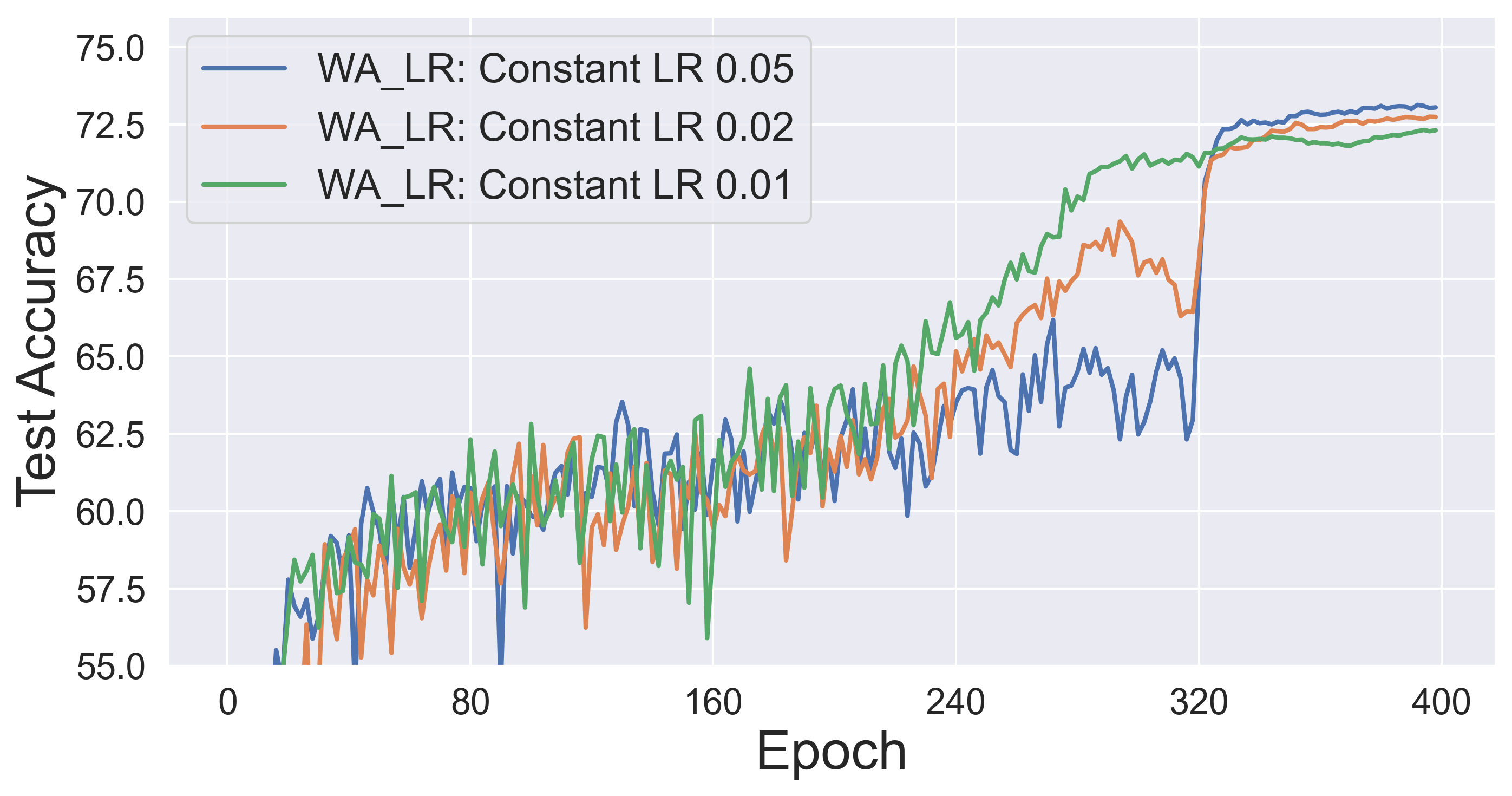
Since offline WA performs averaging at the end of the training process, it requires choosing when to start sampling model checkpoints. A choice that is either too early or too late can be detrimental to the generalization performance of the averaged model. Besides, offline WA uses a cyclical or large constant learning rate scheduler (WA_LR) to sample model checkpoints at the sampling stage. Since the learning rate has a significant impact on the locations of the sampled model checkpoints on the loss surface, the performance of offline WA is sensitive to the choice of WA_LR. As shown in Figure 2, the test accuracy of offline WA varies greatly when different constant learning rates are used at Stage II. With an improper setting, offline WA may even have a negative impact on the generalization performance (e.g., ResNet110 on CIFAR100 in Table II).
To address the issues of offline WA, and combine the advantages of the two types of WA, in this work, we propose a novel weight averaging paradigm named Hierarchical Weight Averaging (HWA) to combine online WA and offline WA within a unified training framework. As illustrated in Figure 1 (c), HWA performs averaging in both online stage and offline stage. During the online stage, HWA trains multiple models in parallel with a normal decaying learning rate scheduler. After each model is evolved for iterations, HWA synchronizes the weights of each model to the averaged weights , and then restarts training.
However, unlike the existing high-frequency online WA, we propose to use low-frequency online WA for HWA, which performs the parameter synchronization operation with a much lower frequency (i.e., larger synchronization period ). In practice, we observe that the low-frequency online WA simulates the ‘restart mechanism’ (e.g. [7]) for DNN training and improves generalization performance.
Later at the offline stage, HWA further takes the average of at different synchronization cycles with a slide window of length , i.e., . Unlike existing offline WA which requires a specific learning rate scheduler and takes the average of all the sampled model checkpoints, our proposed slide-window based offline WA only averages the sampled model checkpoints within the slide window and works well with a regular learning rate scheduler (e.g., a cosine decay of learning rate over the entire budget [7]).
| Training Efficiency | Generalization Performance | |
|---|---|---|
| a: Offline WA | ✗ | ✓ |
| b: Online WA | ✓ | ✗ |
| c: HWA | ✓ | ✓ |
| Rank | cba | cab |
Note that, both online and offline WA is a special case of our proposed HWA. In Table I we also provide a comparison of online WA, offline WA, and our proposed HWA. While online and offline WA can only serve a single purpose, i.e., improving training efficiency or generalization ability, the hybrid paradigm of HWA is able to achieve both of them with better performance. As an example, we plot the top-1 test accuracy of online WA, offline WA, and HWA on CIFAR100 for ResNet56 as a function of training time in Figure 3, where online WA and HWA apply a cosine annealing learning rate throughout the training process, and offline WA starts averaging from the epoch with a constant learning rate.

In sum, the contributions of this work are as follows.
- 1.
We present a novel weight averaging scheme termed Hierarchical Weight Averaging (HWA) which incorporates two different types of WA techniques (i.e., online and offline WA), which are seldom associated with each other, into a unified training framework. By leveraging our designed low-frequency online WA and slide-window based offline WA in a hierarchical manner, HWA achieves several appealing benefits: 1) Unlike online or offline WA, which only serves a single purpose, HWA can improve training efficiency and generalization ability at the same time. 2) HWA outperforms online WA and offline WA in terms of training efficiency and generalization ability, respectively.
- 2.
We also empirically analyze the issues faced by existing offline WA (e.g., the generalization performance is sensitive to the learning rate scheduler (WA_LR)) and how our HWA address them in Section IV.
- 3.
Extensive experiments on CIFAR [2], Tiny-ImageNet [18], CUB200-2011 [19], CalTech256 [20] and ImagenNet [1] have been conducted to demonstrate the effectiveness of the proposed HWA. According to the results, HWA consistently outperforms the other related methods for a variety of architectures. For example, it outperforms the best state-of-the-art competitor by on average across multiple architectures on CIFAR100 dataset. More experimental results could be found in Section V.
The rest of the paper is organized as follows. In Section II, we introduce the related works. Section III gives the detailed procedure of our proposed HWA. In Section V, we discuss how HWA improves the training efficiency and the generalization ability of DNNs. In Section V, we evaluate HWA on several benchmark datasets and compare it with other related methods. Finally, Section VI concludes the paper.
II Related Work
Offline Weight Averaging
Averaging a set of weights traversed by SGD offline can date back several decades in convex optimization [21, 22], but is not typically used to train neural networks. These techniques reduce the impact of noise and improve convergence rates. The Stochastic Weight Averaging (SWA) [15] is proposed to exploit the flatness of training objectives and improve generalization specific to deep learning. Based on the observation that weights of the networks sampled by FGE [23] are on the periphery of the most desirable solutions, SWA [15] creates a network with the averaged weights instead of forming an ensemble. While SGD tends to converge to the boundary of the low-loss region, SWA is able to find a point centered in this region with better generalization.
Following up SWA, various extensions have been proposed for different purposes. SWAG [24] can approximate Bayesian model averaging in Bayesian deep learning and achieves the state-of-the-art uncertainty calibration results in various settings. SWALP [25] can match the performance of full-precision SGD training with quantized parameters. SWAP [26] greatly speeds up the training of neural networks by using large batch sizes. With a different motivation, SWAD [27] and DiWA [28] were proposed to improve the out-of-distribution (OOD) generalization performance of DNNs. In [29], the authors applies WA in the network pruning task.
Online Weight Averaging
The classical parallel mini-batch SGD [30, 16] utilizes distributed hardwares to achieve fast and efficient training of large-scale DNNs. It typically samples gradients of different models in parallel and updates each model’s weights using the averaged gradient in one step. The parallel mini-batch SGD can be interpreted as an online WA, where the local model updates its parameters to the averaged weights at every iteration.
However, this algorithm imposes heavy communication overhead as it requires exchanging of local gradient information at every iteration. To reduce the communication overhead, model averaging techniques [9, 10, 11, 12, 13, 14] suggest performing the weight synchronization operation every iterations. In order to balance the communication overhead and convergence speed, the value of parameter synchronization period considered in these works is also relatively small, (e.g., in [9], in [12], in [17]). One extreme case is the one-shot averaging [14], where weights are averaged only at the last iteration but may yield inaccurate solutions for certain non-convex optimization [12]. Theoretical analysis of the convergence speed of online WA could be found in [31, 13, 17]. While existing offline/online WA methods perform either offline parameter averaging or online parameter averaging, HWA performs both of them during the training procedure.
Other Related Works
The Lookahead optimizer [32] maintains a set of slow weights and fast weights, and updates the slow weights with the fast weights every steps. The stochastic gradient descent with restarts (SGDR) [7] first introduces the idea of scheduling the learning rate cyclically as a modification to the common linear or step-wise decay strategy. Some studies [23] point out that SGDR can escape from local minimum and explore other regions. Recently, a training strategy named Improved Training of Convolutional Filters (RePr) [33] was proposed to improve the network on the filter level. RePr first freezes the overlapped filters to train the sub-network, and then restores the frozen filters and continues to train the full network. With a similar motivation, Filter Grafting (FG) [34] uses entropy-based criteria to measure the information of filters and grafts external information from other networks trained in parallel into invalid filters. SAM [35] is a novel optimizer that improves model generalization by simultaneously minimizing loss value and loss sharpness.
III Detailed Procedure of HWA
In this section, we introduce the detailed procedure of HWA and leave the analysis of how HWA works in Section IV. The general idea of HWA is given in Figure 1(c). In Algorithm 1 and 2, we also provide the pseudo-code of the online and offline modules of HWA, respectively.
III-A Online Module of HWA
At the online stage, HWA trains models in parallel with different sampling orders. A standard SGD optimizer with a regular decaying learning rate scheduler is used to evolve each model by performing sequential SGD updates to batches of training examples sampled from the dataset :
| where |
Here is the loss function, and denotes averaging or synchronization cycle. After each model is updated for iterations (), HWA takes the average of the weights of the models in parallel to obtain the averaged weights for the synchronization cycle
Once completed, it synchronizes the weights of each model at the start of the next synchronization cycle to the averaged weights
Since is updated within a synchronization cycle and is calculated outside of a synchronization cycle, we name them Inner Weights and Outer Weights, respectively.
for to do 1
( step in the synchronization cycle)
2
if then 4
Save checkpoint
for k = 1 to do 5
III-B Offline Module of HWA
At the offline stage, HWA also further averages the outer weights saved at different synchronization cycles during the online stage. Unlike offline WA, HWA does not require a large constant or cyclical learning rate at the end of the training process. From our experiments, we find it works well with a regular decaying learning rate scheduler over the entire budget, e.g., a cosine decay or linear decay.
While offline WA averages all the model checkpoints sampled from the time it starts averaging, HWA uses a slide window with a length of and takes the average of outer weights at different synchronization cycles within the window.
In practice, the offline WA module does not necessarily average all the outer weights within the slide window. For example, it can take the average of outer weights with index in multiples of a particular integer, e.g., . Besides, when we have sufficient training budget, we can try multiple possible as the length of slide window also has a significant impact on the performance of the final averaged model .
Update batch normalization statistics if the DNN uses batch normalization
IV How HWA Works?
In this section, we discuss how HWA improves the training efficiency and generalization ability of DNNs.
IV-A Convergence Condition of SGD
In order to study how HWA improves SGD, here we first derive the convergence condition of SGD. Let denote the empirical risk of model and denote a single training sample. Suppose the batch size is , then the gradient of a batch of samples is
On the assumption of Lipschitz-continuous gradient with Lipschitz constant and the update at each iteration is , we have
Suppose denotes the variable of mini-batch samples, the empirical risk is expected to decrease if
For a fixed dataset and model , the right hand side is determined by the learning rate , and left hand side is controlled by the batch size. As long as the learning rate stays constant, model would converge only if the mini-batch gradient estimates accurately enough.

Therefore, with a constant learning rate , the optimizer would converge to a certain point and then start to oscillate and explore around the minima. This phenomenon is clearly shown in Figure 4, where we plot the training and test accuracy of ResNet20 on CIFAR100 when it is trained by SGD with a constant learning rate . As we can see, the training and test accuracy start to oscillate after dozens of epochs, which indicates that the optimizer is exploring around the local minima instead of progressing to the local minima.
IV-B How HWA Improves Training Efficiency
Though the loss functions of DNNs are known to be nonconvex [36], the loss surfaces over the trajectory of SGD are approximately convex [37]. According to the convergence condition, SGD would oscillate and explore around the local minima after it converges to a certain point unless the learning rate further decays. Therefore, by taking the average of the weights of multiple model checkpoints, the averaged solution would quickly progress to a point closer to the minima with training lower loss.
This scenario is shown in Figure 5, where we use the visualization tool [38] to project model checkpoint and (two models in parallel) and their corresponding averaged weights on the training loss surface of ResNet32 on CIFAR100. Note that, and are evolved by SGD for steps (one epoch) from the same starting point , and hence they are within the same local minima. Through the online averaging operation, the averaged solution immediately reaches a location closer to the minima on the training loss surface.
Similar to the online averaging operation of HWA, the offline averaging operation of HWA also speeds up convergence in a similar way. However as the offline averaging operation of HWA is performed vertically at different synchronization cycles on top of the outer weights obtained during the online stage, the HWA weights progresses to a point closer to the minima than . To show this scenario, we also use the visualization tool [38] to project the offline averaging operation of HWA in Figure 6.

Therefore, by performing the weight averaging operations in both horizontal and vertical directions hierarchically, HWA can progress to the local minima more quickly than online WA alone, which only performs the averaging operation horizontally. In Figure 7, we plot the top-1 test accuracy and test loss of Inner Weights , Outer Weights , and HWA Weights for ResNet32 on CIFAR10 and CIFAR100, where the synchronization period is (i.e., one epoch) and the length of slide window is . As we can observe, the HWA Weights achieves faster convergence than Outer Weights and inner weights .

IV-C How HWA Improves Generalization Ability
One popular hypothesis about the generalization ability11 1 In this paper, we refer to generalization ability as the ability in predicting unseen, in-distribution data (e.g., test data). of DNNs [39, 40, 15] is that the generalization performance of DNNs is correlated with the flatness of its local minima, and a sharp local minimum typically tends to generalize worse than the flat ones [41]. While most existing works (e.g., [15, 42]) attribute the better generalization ability of neural networks to a wider local minimum, the location to which a network converges within a local minimum also greatly affects the generalization performance. As observed in [43], the loss landscape of local minima is asymmetric and exists both sharp and flat directions, and the solution locates at the flat side has better generalization performance due to the random shift between the training loss and test loss.
According to the convergence condition of SGD, when the model checkpoints are sampled with the same learning rate, they would be distributed around the local minima with similar empirical risks (refer to Figure 4). As a result, as illustrated in Figure 8, the averaged model tends to be biased to the flat side of the local minima. Due to the shift between the training and test loss, the averaged model has better generalization ability than the model with the minimal training loss. Such an example is shown in Figure 9, which plots the accuracy and loss of ResNet20 on CIFAR100 along the direction between an averaged model (location ) and an individual model (location ). Apparently, all the models between and are in the same local minima because there is no sharp drop in training and test accuracy. Despite the lower training accuracy, the averaged model achieves higher test accuracy than the individual model, because it is biased to the flat side of the loss landscape. This also implies that the training accuracy is a poor indicator of the generalization ability.
Figure 8 also explains why offline WA is sensitive to the choice of learning rate used to sample model checkpoints. According to the convergence condition of SGD, the learning rate determines the empirical risk or loss of the sampled model checkpoints (refer to Figure 4) and hence their locations on the loss landscape. Since the averaged model is obtained by taking the average of these model checkpoints, its location within the local minima is also determined by the learning rate with which these model checkpoints are sampled. As a result, a choice of learning rate that is either too small or too large can be detrimental to the performance of offline WA, which leverages a large constant or cyclical learning rate to sample model checkpoints. For example in Figure 8, the averaged model obtained with an intermediate learning rate achieves the best test performance.

Unlike offline WA, as illustrated in Figure 10, HWA takes the average of model checkpoints sampled with different learning rates with a slide window of length . As a result, the averaged model at different synchronization cycles is located at different positions with different distances to the minima of the training loss surface. Compared to offline WA, HWA is able to explore more locations on the flat side of the local minima and hence is more likely to find a better averaged model.
Note that, the averaged model at the last synchronization cycle does not necessarily be the best averaged model. For example, as illustrated in Figure 10, the best averaged model is obtained at the synchronization cycle. We also plot the training and test accuracy of as a function of epochs for ResNet110 on CIFAR100 in Figure 11, where the synchronization period is one epoch and the length of slide window . As we can observe, the averaged model around the synchronization cycle achieves the best test accuracy. Therefore, in practice, we use techniques such as early stopping to obtain the best averaged model.

Though the averaged model with the minimal training loss does not necessarily be the averaged model with the best validation performance, in most cases, the best averaged model is located close to the minima of the training loss. Therefore, it is important for the optimizer to explore more locations close to the minima of the training loss. With the help of the online WA module, HWA progresses to the regions close to the minima of training loss more quickly than naive offline WA, which as a result, helps it to find a better averaged model.
Discussion: The ‘restart’ mechanism [7, 8], which switches the status of a model to a lower fitting level to the training data (i.e., higher training loss), is claimed to achieve a longer-term beneficial effect on generalization performance at the cost of short term benefit. While existing techniques [7, 8] restart the training by increasing the learning rate, we observe that the online averaging module of HWA also achieves a similar ‘restart’ effect. We observe that, in general, the loss of the averaged model decreases over training time. However, within a synchronization cycle, the loss of inner weights would surprisingly increase with iteration times . For example, as shown in Figure 12, after each model is updated by the optimizer for steps (), the training loss increases instead of decreasing.

Note that the online averaging operation of HWA would result in a significant decrease in the empirical risk, i.e.,
As a result, the convergence condition at the start of the synchronization cycle does not hold any more for , and the optimizer would receive more noise information than gradient information within the synchronization cycle. That’s why the empirical risk increases in general with the iteration times within a synchronization cycle.
While there is no consensus on how the ‘restart’ mechanism improves the training of DNNs, we provide a possible explanation to the success of the ‘restart’ mechanism: A neural network tends to generalize easy training samples and memorizes the “hard” samples through the massive parameters. Once the hard samples are memorized, their losses would decrease to zero quickly, and hence the network overfits the hard samples. On the other hand, restart techniques switch the network status back to a lower fitting level, and hence the hard samples memorized by the network are more likely to be forgotten.
V Experiment
| Method | Dataset | ResNet20 | ResNet32 | ResNet56 | ResNet110 | VGG16 | MobileNetV2 |
|---|---|---|---|---|---|---|---|
| Baseline | CIFAR10 | 91.60 | 92.60 | 93.50 | 93.81 | 93.25 | 93.89 |
| CA | 92.51 | 93.09 | 93.60 | 93.91 | 94.01 | 94.11 | |
| SWA | 92.67 | 93.38 | 93.75 | 94.17 | 94.18 | 94.80 | |
| RePr [33] | 93.10 | 93.90 | - | 94.60 | - | - | |
| FG [34] | 92.98 | 93.94 | 94.73 | 94.96 | 94.26 | 95.03 | |
| SAM [35] | 93.09 | 94.06 | 94.78 | 95.01 | 94.62 | 95.35 | |
| HWA | 93.46 | 94.41 | 94.96 | 95.19 | 94.88 | 95.46 | |
| Baseline | CIFAR100 | 67.40 | 69.82 | 71.55 | 73.21 | 72.55 | 73.39 |
| CA | 68.53 | 70.71 | 72.03 | 72.98 | 74.15 | 74.30 | |
| SWA | 69.03 | 70.20 | 73.02 | 71.57 | 73.92 | 76.90 | |
| RePr [33] | 68.90 | 69.90 | - | 73.60 | - | - | |
| FG [34] | 68.84 | 71.28 | 72.83 | 75.27 | 74.63 | 76.30 | |
| SAM [35] | 69.75 | 72.69 | 74.06 | 75.17 | 75.59 | 77.37 | |
| HWA | 70.79 | 73.15 | 75.61 | 76.68 | 77.12 | 78.31 |
In this section, we evaluate our HWA on several benchmark datasets CIFAR10 and CIFAR100 [2], Tiny-ImageNet [44], CUB200-2011 [19], CalTech256 [20] and ImageNet [1], and also compare it with other related methods.
The two CIFAR datasets consist of images with a resolution of . CIFAR10 contains 10 classes and CIFAR100 contains 100 classes. Both datasets contain a train set of images and a test set of images. Tiny-ImageNet [44] comprises colored images over classes with a resolution of . The CUB-200-2011 contains images of categories belonging to birds. The CalTech256 is an object recognition dataset comprising real-world images with different sizes over 256 object classes and an additional clutter class. Imagenet is an image classification dataset with over 1.3 million images and contains 1000 classes.
In particular, the following methods are involved in the experiments.
- 1.
Baseline: the conventional SGD with step-wise learning rate decay ( at every epochs).
- 2.
CA: the cosine learning rate strategy, which is claimed to outperform other learning rate schedulers.
- 3.
FG: filter grafting for deep neural networks [34].
- 4.
RePr: improved training of convolutional filters [33].
- 5.
SWA: stochastic weight averaging (i.e., offline WA).
- 6.
SAM: shareness-aware minimization [35].
- 7.
HWA: our proposed HWA algorithm with default synchronization period , where is the number of training samples and is the batch size.
Among the above mentioned techniques, SWA is the primary work we aim to compare because both HWA and SWA are weight averaging strategies.
V-A Comparison with Other Methods
In this section, we experimentally compare our HWA with other methods on CIFAR10 and CIFAR100 datasets in Table II22 2 The experimental results of RePr [33] reported in Table II come from the corresponding paper because the code of RePr [33] is not publicly available. ‘–’ denotes the result is not reported in the corresponding paper. For SWA [15] and FG [45], the experiments are conducted in our implementation using the code provided by the original group.. We use bold font to highlight the best accuracy and blue color to denote the second-best result. For CIFAR, we evaluate our HWA on three popular networks: VGG, ResNet and MobileNetV2. All the networks are trained by SGD with a momentum of 0.9 and a weight decay of . A cosine learning rate strategy over the whole budget is used by default. The initial learning rate is set to 0.1 for ResNets and VGG, and 0.05 for MoibleNetV2.
The results in Table II demonstrate that HWA achieves the best performance among all the training schemes. On average, it improves the baseline by around on CIFAR10 and on CIFAR100. In particular, it outperforms the method with the second-best accuracy by on CIFAR100 on average. Compared to SWA, the performance of HWA is more stable. For example, the test accuracy of SWA is even lower than the baseline on CIFAR100 for ResNet110. On the other hand, with the same experiment setting, SWA achieves the second-best results for ResNet20, ResNet56 and MobileNetV2. These results also support our claim that SWA is sensitive to the learning rate scheduler at the sampling stage.
| Dataset | Method | ResNet20 | ResNet32 | ResNet56 |
|---|---|---|---|---|
| CIFAR10 | Baseline | 91.60 | 92.60 | 93.60 |
| +CA | 92.51 | 93.09 | 93.60 | |
| +online module | 92.98 | 93.98 | 94.49 | |
| +offline module | 93.46 | 94.41 | 94.96 | |
| Method | ResNet110 | VGG16 | MobileNetV2 | |
| CIFAR10 | Baseline | 93.81 | 93.25 | 93.89 |
| +CA | 93.91 | 94.01 | 94.11 | |
| +online module | 94.55 | 94.57 | 95.22 | |
| +offline module | 95.19 | 94.88 | 95.46 | |
| Method | ResNet20 | ResNet32 | ResNet56 | |
| CIFAR100 | Baseline | 67.40 | 69.82 | 71.55 |
| + CA | 68.53 | 70.71 | 72.03 | |
| +online module | 69.42 | 70.91 | 73.30 | |
| +offline module | 70.79 | 73.15 | 75.61 | |
| Method | ResNet110 | VGG16 | MobileNetV2 | |
| CIFAR100 | Baseline | 73.21 | 72.55 | 73.39 |
| +CA | 72.98 | 74.15 | 74.30 | |
| +online module | 75.37 | 75.92 | 76.28 | |
| +offline module | 76.68 | 77.12 | 78.31 |

V-B Contribution of Online and Offline WA Module
Both the online and offline WA module of HWA can improve the generalization performance of DNNs. In Table III, we report the contributions of the online WA module of HWA and the additional improvement from the offline WA module. On average, the online WA module provides an improvement around and on CIFAR10 and CIFAR100, respectively. By applying the offline WA module, we obtain an additional improvement around and on CIFAR10 and CIFAR100, respectively.
As we can observe, the performance of the online WA module is not stable when we apply it alone. For example, it provides almost no notable improvement for ResNet32 on CIFAR100. However, by additionally applying the offline WA module, HWA outperforms CA by around . On the other hand, the online WA module of HWA improves CA by about for MobileNetV2 on CIFAR10. However, the additional gain in test accuracy from the offline WA module is negligible (around ). In sum, the hybrid of online and offline WA can improve the stability of HWA.
V-C Number of Models in Parallel
In this section, we explore how the number of models in parallel affects the final generalization performance of HWA. In Table IV, we report the test accuracy of HWA on CIFAR10 and CIFAR100 with varying numbers of models trained in parallel during the online stage. As we can observe, though the best test accuracy is achieved when the number of models in parallel is or , the improvement in test accuracy is not very notable as increases from to . Thus, in practice, we can simply set when there is a limited training budget.
| Data | 2 | 3 | 4 | |
|---|---|---|---|---|
| CIFAR100 | ResNet20 | 70.79 | 71.13 | 70.58 |
| ResNet32 | 73.15 | 72.93 | 73.19 | |
| CIFAR10 | ResNet20 | 93.46 | 93.49 | 93.43 |
| ResNet32 | 94.41 | 94.37 | 94.53 |
V-D Slide Window Length
In this section, we conduct several ablation experiments on CIFAR10 and CIFAR100 with ResNet20 and ResNet32 to study the influence from the length of slide window. Each experiment is repeated times and a slide window with length of or is considered in the experiment. In Figure 13, we present the box-plot of the experimental results. As we can observe, the length of the slide window would exert different influences on the test accuracy for different datasets. Therefore, we may achieve further improvement by choosing a suitable slide window length for different datasets and architectures for the offline WA module of HWA.

V-E Results on Other Datasets
In this section, we evaluate our proposed HWA on several other datasets: Tiny-ImageNet, CUB200-2011 [19], CalTech256 [20] and ImageNet [1]. We use the models implemented in Torchvision in the experiment. For comparison, we also report the experimental results of the baseline and SWA, which is the primary technique we aim to compare. Unless mentioned otherwise, the experiment setting for CIFAR is also used in these experiments.
Tiny-ImageNet: In Table V we show the top-1 test accuracy on Tiny-ImageNet, which comprises colored images over classes with a resolution of . In the training process, a crop is randomly sampled from the original image or its horizontal flip with a padding size of . The initial learning rate is for ResNet18 and for MobileNetV2 and ShuffleNetV2.
| Model | ResNet18 | MobileNetV2 | ShuffleNetV2 |
|---|---|---|---|
| Baseline | 53.18 | 49.94 | 46.52 |
| SWA | 54.70 | 48.92 | 47.20 |
| SAM | 55.24 | 51.82 | 47.62 |
| HWA | 57.10 | 53.16 | 49.34 |
CUB200-2011: Table VI shows the top-1 test accuracy of different models on CUB200-2011, which contains images of categories belonging to birds. During training, a crop is randomly sampled from the original image or its horizontal flip and no other data augmentation is applied. The initial learning rate is for all models.
| Model | ResNet18 | MobileNetV2 | ShuffleNetV2 |
|---|---|---|---|
| Baseline | 58.76 | 62.43 | 58.92 |
| SWA | 63.41 | 64.63 | 60.96 |
| SAM | 60.31 | 63.08 | 59.90 |
| HWA | 65.12 | 69.44 | 65.44 |
CalTech256: In Table VII we report the top-1 test accuracy on CalTech256, an object recognition dataset comprising real-world images with different sizes over object classes and an additional clutter class. The experiment setting for CalTech256 is the same as CUB200-2011 except that the initial learning rate is for all architectures.
| Model | ResNet18 | MobileNetV2 | ShuffleNetV2 |
|---|---|---|---|
| Baseline | 64.59 | 66.30 | 62.50 |
| SWA | 68.30 | 68.39 | 64.37 |
| SAM | 66.43 | 67.28 | 63.73 |
| HWA | 69.33 | 69.55 | 67.20 |
Compared to CIFAR, these datasets are more difficult as they have fewer training samples and more classes. As we can observe from Table V, VI and VII, our HWA outperforms the baseline and SWA consistently across these datasets and architectures, which demonstrates the effectiveness of HWA in these more difficult classification tasks.
ImageNet We also evaluate HWA on ImageNet [1], a large-scale image dataset with over million images of classes. In the experiment, each model is trained with a batch size of for epochs by SGD with a momentum of and a weight decay of . During training, a random resize and crop of and random horizontal flip are performed as data augmentation. For ResNet50, we also apply the cutout regularization [46] in the training process.
In Table VIII, we report the top-1 and top-5 test accuracy of each method on ImageNet. As we can observe, HWA outperforms the baseline and SWA by and for ResNet50, respectively. Therefore, the experimental results on ImageNet verify that HWA also works well in the large-scale image classification task.
| Baseline | SWA | SAM | HWA | |
|---|---|---|---|---|
| Top-1 | 76.67 | 76.97 | 77.11 | 77.72 |
| Top-5 | 93.21 | 93.41 | 93.54 | 93.78 |
V-F Faster Convergence
In Section IV-B, we show that HWA improves the convergence speed by performing the weight averaging operation in both horizontal and vertical directions hierarchically. For example, as we can observe in Figure 3 and 7, HWA converges much faster than online WA and offline WA alone. In Figure 14, we provide more similar experimental results for different architectures (i.e., VGG16, MobileNetV2 and ResNet110) on CIFAR100. For HWA, the synchronization period is and the slide window length is . As we can observe, HWA converges much faster than the baseline with the same optimizer and learning rate scheduler.
VI Conclusion
In this work, we propose a novel training paradigm called hierarchical weight averaging (HWA), which incorporates the online WA and offline WA into a unified training framework. Unlike online or offline WA, which only serves a single purpose, i.e., improving training efficiency or generalization ability, the hybrid paradigm of HWA is able to achieve both of them with better performance. By performing the weight averaging operations in both horizontal and vertical directions hierarchically, HWA outperforms online WA and offline WA alone. We also analyze how HWA improves the training efficiency and generalization ability of DNNs from the perspective of the loss landscape of DNNs. Finally, extensive experimental results demonstrate the effectiveness of the proposed HWA.
References
- Krizhevsky et al. [2012] A. Krizhevsky, I. Sutskever, and G. E. Hinton, “Imagenet classification with deep convolutional neural networks,” in Advances in neural information processing systems, 2012, pp. 1097–1105.
- Krizhevsky et al. [2009] A. Krizhevsky, G. Hinton et al., “Learning multiple layers of features from tiny images,” 2009.
- Donahue et al. [2014] J. Donahue, Y. Jia, O. Vinyals, J. Hoffman, N. Zhang, E. Tzeng, and T. Darrell, “Decaf: A deep convolutional activation feature for generic visual recognition,” in International conference on machine learning, 2014, pp. 647–655.
- Long et al. [2015] J. Long, E. Shelhamer, and T. Darrell, “Fully convolutional networks for semantic segmentation,” in Proceedings of the IEEE conference on computer vision and pattern recognition, 2015, pp. 3431–3440.
- Hackel et al. [2017] T. Hackel, N. Savinov, L. Ladicky, J. D. Wegner, K. Schindler, and M. Pollefeys, “Semantic3d. net: A new large-scale point cloud classification benchmark,” arXiv preprint arXiv:1704.03847, 2017.
- Duchi et al. [2011] J. Duchi, E. Hazan, and Y. Singer, “Adaptive subgradient methods for online learning and stochastic optimization.” Journal of machine learning research, vol. 12, no. 7, 2011.
- Loshchilov and Hutter [2016] I. Loshchilov and F. Hutter, “Sgdr: Stochastic gradient descent with warm restarts,” arXiv preprint arXiv:1608.03983, 2016.
- Smith [2017] L. N. Smith, “Cyclical learning rates for training neural networks,” in 2017 IEEE Winter Conference on Applications of Computer Vision (WACV). IEEE, 2017, pp. 464–472.
- Lin et al. [2018] T. Lin, S. U. Stich, K. K. Patel, and M. Jaggi, “Don’t use large mini-batches, use local sgd,” arXiv preprint arXiv:1808.07217, 2018.
- McMahan et al. [2017] B. McMahan, E. Moore, D. Ramage, S. Hampson, and B. A. y Arcas, “Communication-efficient learning of deep networks from decentralized data,” in Artificial Intelligence and Statistics. PMLR, 2017, pp. 1273–1282.
- Mcdonald et al. [2009] R. Mcdonald, M. Mohri, N. Silberman, D. Walker, and G. S. Mann, “Efficient large-scale distributed training of conditional maximum entropy models,” in Advances in neural information processing systems, 2009, pp. 1231–1239.
- Zhang et al. [2016] J. Zhang, C. De Sa, I. Mitliagkas, and C. Ré, “Parallel sgd: When does averaging help?” arXiv preprint arXiv:1606.07365, 2016.
- Stich [2018] S. U. Stich, “Local sgd converges fast and communicates little,” arXiv preprint arXiv:1805.09767, 2018.
- Zinkevich et al. [2010] M. Zinkevich, M. Weimer, L. Li, and A. J. Smola, “Parallelized stochastic gradient descent,” in Advances in neural information processing systems, 2010, pp. 2595–2603.
- Izmailov et al. [2018] P. Izmailov, D. Podoprikhin, T. Garipov, D. Vetrov, and A. G. Wilson, “Averaging weights leads to wider optima and better generalization,” arXiv preprint arXiv:1803.05407, 2018.
- Li et al. [2014] M. Li, D. G. Andersen, A. J. Smola, and K. Yu, “Communication efficient distributed machine learning with the parameter server,” in Advances in Neural Information Processing Systems, 2014, pp. 19–27.
- Yu et al. [2019] H. Yu, S. Yang, and S. Zhu, “Parallel restarted sgd with faster convergence and less communication: Demystifying why model averaging works for deep learning,” in Proceedings of the AAAI Conference on Artificial Intelligence, vol. 33, 2019, pp. 5693–5700.
- Deng et al. [2009] J. Deng, W. Dong, R. Socher, L.-J. Li, K. Li, and L. Fei-Fei, “Imagenet: A large-scale hierarchical image database,” in 2009 IEEE conference on computer vision and pattern recognition. Ieee, 2009, pp. 248–255.
- Wah et al. [2011] C. Wah, S. Branson, P. Welinder, P. Perona, and S. Belongie, “The caltech-ucsd birds-200-2011 dataset,” 2011.
- Griffin et al. [2007] G. Griffin, A. Holub, and P. Perona, “Caltech-256 object category dataset,” 2007.
- Ruppert [1988] D. Ruppert, “Efficient estimations from a slowly convergent robbins-monro process,” Cornell University Operations Research and Industrial Engineering, Tech. Rep., 1988.
- Polyak and Juditsky [1992] B. T. Polyak and A. B. Juditsky, “Acceleration of stochastic approximation by averaging,” SIAM journal on control and optimization, vol. 30, no. 4, pp. 838–855, 1992.
- Huang et al. [2017] G. Huang, Y. Li, G. Pleiss, Z. Liu, J. E. Hopcroft, and K. Q. Weinberger, “Snapshot ensembles: Train 1, get m for free,” arXiv preprint arXiv:1704.00109, 2017.
- Maddox et al. [2019] W. J. Maddox, P. Izmailov, T. Garipov, D. P. Vetrov, and A. G. Wilson, “A simple baseline for bayesian uncertainty in deep learning,” in Advances in Neural Information Processing Systems, 2019, pp. 13 153–13 164.
- Yang et al. [2019] G. Yang, T. Zhang, P. Kirichenko, J. Bai, A. G. Wilson, and C. De Sa, “Swalp: Stochastic weight averaging in low-precision training,” arXiv preprint arXiv:1904.11943, 2019.
- Gupta et al. [2020] V. Gupta, S. A. Serrano, and D. DeCoste, “Stochastic weight averaging in parallel: Large-batch training that generalizes well,” arXiv preprint arXiv:2001.02312, 2020.
- Cha et al. [2021] J. Cha, S. Chun, K. Lee, H.-C. Cho, S. Park, Y. Lee, and S. Park, “Swad: Domain generalization by seeking flat minima,” Advances in Neural Information Processing Systems, vol. 34, pp. 22 405–22 418, 2021.
- Rame et al. [2022] A. Rame, M. Kirchmeyer, T. Rahier, A. Rakotomamonjy, P. Gallinari, and M. Cord, “Diverse weight averaging for out-of-distribution generalization,” arXiv preprint arXiv:2205.09739, 2022.
- Wang et al. [2021] Y. Wang, H. Park, and J. Lee, “Memory-free stochastic weight averaging by one-way variational pruning,” IEEE Signal Processing Letters, vol. 28, pp. 1021–1025, 2021.
- Dekel et al. [2012] O. Dekel, R. Gilad-Bachrach, O. Shamir, and L. Xiao, “Optimal distributed online prediction using mini-batches,” The Journal of Machine Learning Research, vol. 13, pp. 165–202, 2012.
- Zhou and Cong [2017] F. Zhou and G. Cong, “On the convergence properties of a -step averaging stochastic gradient descent algorithm for nonconvex optimization,” arXiv preprint arXiv:1708.01012, 2017.
- Zhang et al. [2019a] M. Zhang, J. Lucas, J. Ba, and G. E. Hinton, “Lookahead optimizer: k steps forward, 1 step back,” in Advances in Neural Information Processing Systems, 2019, pp. 9597–9608.
- Prakash et al. [2019] A. Prakash, J. Storer, D. Florencio, and C. Zhang, “Repr: Improved training of convolutional filters,” in Proceedings of the IEEE conference on computer vision and pattern recognition, 2019, pp. 10 666–10 675.
- Meng et al. [2020a] F. Meng, H. Cheng, K. Li, Z. Xu, R. Ji, X. Sun, and G. Lu, “Filter grafting for deep neural networks,” in Proceedings of the IEEE/CVF Conference on Computer Vision and Pattern Recognition, 2020, pp. 6599–6607.
- Foret et al. [2020] P. Foret, A. Kleiner, H. Mobahi, and B. Neyshabur, “Sharpness-aware minimization for efficiently improving generalization,” arXiv preprint arXiv:2010.01412, 2020.
- Choromanska et al. [2015] A. Choromanska, M. Henaff, M. Mathieu, G. B. Arous, and Y. LeCun, “The loss surfaces of multilayer networks,” in Artificial intelligence and statistics. PMLR, 2015, pp. 192–204.
- Goodfellow et al. [2014] I. J. Goodfellow, O. Vinyals, and A. M. Saxe, “Qualitatively characterizing neural network optimization problems,” arXiv preprint arXiv:1412.6544, 2014.
- Li et al. [2018] H. Li, Z. Xu, G. Taylor, C. Studer, and T. Goldstein, “Visualizing the loss landscape of neural nets,” in Advances in Neural Information Processing Systems, 2018, pp. 6389–6399.
- Cooper [2018] Y. Cooper, “The loss landscape of overparameterized neural networks,” arXiv preprint arXiv:1804.10200, 2018.
- Draxler et al. [2018] F. Draxler, K. Veschgini, M. Salmhofer, and F. Hamprecht, “Essentially no barriers in neural network energy landscape,” in International conference on machine learning. PMLR, 2018, pp. 1309–1318.
- Keskar et al. [2016] N. S. Keskar, D. Mudigere, J. Nocedal, M. Smelyanskiy, and P. T. P. Tang, “On large-batch training for deep learning: Generalization gap and sharp minima,” arXiv preprint arXiv:1609.04836, 2016.
- Zhang et al. [2019b] L. Zhang, J. Song, A. Gao, J. Chen, C. Bao, and K. Ma, “Be your own teacher: Improve the performance of convolutional neural networks via self distillation,” in Proceedings of the IEEE/CVF International Conference on Computer Vision, 2019, pp. 3713–3722.
- He et al. [2019] H. He, G. Huang, and Y. Yuan, “Asymmetric valleys: Beyond sharp and flat local minima,” arXiv preprint arXiv:1902.00744, 2019.
- Yao and Miller [2015] L. Yao and J. Miller, “Tiny imagenet classification with convolutional neural networks,” CS 231N, vol. 2, no. 5, p. 8, 2015.
- Meng et al. [2020b] F. Meng, H. Cheng, K. Li, Z. Xu, R. Ji, X. Sun, and G. Lu, “Code of Filter Grafting,” https://github.com/fxmeng/filter-grafting, 2020.
- DeVries and Taylor [2017] T. DeVries and G. W. Taylor, “Improved regularization of convolutional neural networks with cutout,” arXiv preprint arXiv:1708.04552, 2017.