Lookahead Diffusion Probabilistic Models for Refining Mean Estimation

Suppose we have a set of observations of $\boldsymbol{x}$ that are drawn from a data distribution $q(\boldsymbol{x})$. A forward diffusion process can be defined as a sequence of increasingly noisy versions $\boldsymbol{z}_{t}$, $t\in[0,1]$, of $\boldsymbol{x}$, where $\boldsymbol{z}_{t=1}$ indicates the noisiest version (we will discretize $t$ later on). For a Gaussian-driven process, the latent variable $\boldsymbol{z}_{t}$ can be represented in terms of $\boldsymbol{x}$ being contaminated by a Gaussian noise as

where $\boldsymbol{\epsilon}_{t}\sim\mathcal{N}(0,\boldsymbol{I})$, and $\alpha_{t}$ and $\sigma_{t}$ are strictly positive scalar-valued functions of $t$, and $\boldsymbol{I}$ is the identity matrix. To formalise the notion of $\boldsymbol{z}_{t}$ being increasingly noisy, $\boldsymbol{z}_{t}$ can be alternatively represented in terms of $\boldsymbol{z}_{s}$, $s<t$, as

where $\boldsymbol{\epsilon}_{t|s}$ is the additional Gaussian noise being added to a scaled version of $\boldsymbol{z}_{s}$, and $(\alpha_{t|s},\sigma_{t|s}^{2})$ are given by

where the conditional variance $\sigma_{t|s}^{2}$ is assume to be positive, i.e., $\sigma_{t|s}^{2}>0$. One major advantage of the above formulation is that it includes both the variance-preserving process with $\alpha_{t}=\sqrt{1-\sigma_{t}^{2}}$ Dickstein15DPM; Ho20DDPM and variance-exploding process with $\alpha_{t}=1$ Song19; Song21SDE_gen.

It is immediate that the process (1)-(3) is Markov. That is, the conditional distribution $q(\boldsymbol{z}_{u}|\boldsymbol{z}_{t},\boldsymbol{z}_{s})=q(\boldsymbol{z}_{u}|\boldsymbol{z}_{t})=\mathcal{N}(\alpha_{u|t}\boldsymbol{z}_{t},\sigma_{u|t}^{2}\boldsymbol{I})$, where $0\leq s<t<u\leq 1$. Consequently, it can be shown that $q(\boldsymbol{z}_{s}|\boldsymbol{z}_{t},\boldsymbol{x})$, $s<t$, is Normal distributed by using Bayes rule (see Appendix A of Kingma21DDPM),

As will be discussed later on, the backward process heavily relies on the relation between $(\boldsymbol{z}_{t},\boldsymbol{x})$ and $\boldsymbol{z_{s}}$ in the formulation (4).

As one example, the above process includes the forward process of a DDPM as a special case. One can simply discretize $t\in[0,1]$ into $N$ uniform timesteps, i.e., $t_{i}=i/N$, and let $\{\alpha_{t_{i}}=\sqrt{1-\sigma_{t_{i}}^{2}}|N\geq i\geq 0\}$ be a strictly decreasing sequence.

In general, a backward process is designed to reverse the forward process introduced earlier for the purpose of approximating the data distribution $q(\boldsymbol{x})$. Without loss of generality, we denote a discrete backward process as

where the support region $[0,1]$ for $t$ is discretized into $N$ uniform timesteps, i.e., $t_{i}=i/N$, and $t_{i}$ is replaced by $i$ to simplify notation. The objective is to find a specific form of the backward process such that its marginal distribution with regard to $\boldsymbol{x}$ approaches $q(\boldsymbol{x})$:

To facilitate computation, DDPM makes the following approximation to the backward process of (4):

where $\alpha_{i|i-1}$ and $\sigma^{2}_{i|i-1}$ follow from (3) with $(t,s)=(i/N,(i-1)/N)$, and $\hat{\boldsymbol{x}}(\boldsymbol{z}_{i},i)$ denotes the predicted sample for $\boldsymbol{x}$ by using $\boldsymbol{z}_{i}$ and timestep $i$. The marginal distribution of $\boldsymbol{z}_{N}$ is approximated to be a spherical Gaussian, i.e., $p(\boldsymbol{z}_{N})\approx p(0,\beta\boldsymbol{I})$, where $\beta=1$ for variance-preserving DPMs. A nice property of (8) is that the conditional distribution is Gaussian. As a result, the computation in the backward process only needs to focus on a sequence of means $\boldsymbol{\mu}(\boldsymbol{z}_{i-1}|\boldsymbol{z}_{i},i)$ and variances $\varphi_{i}$ from $i=N$ to $i=0$.

Next, we briefly discuss the computation for $\hat{\boldsymbol{x}}(\boldsymbol{z}_{i},i)$ in Ho20DDPM, which is followed by recent, more advanced, DPM models such as DDIM Song21DDIM and DPM-Solver Lu22DPM_Solver. In Ho20DDPM, a DNN model $\hat{\boldsymbol{\epsilon}}_{\boldsymbol{\theta}}$ is designed to make a direct prediction of the added Gaussian noise $\boldsymbol{\epsilon}_{t}$ to $\boldsymbol{x}$ in a latent variable $\boldsymbol{z}_{t}$ of (1). In particular, the model is trained to minimize a summation of expected squared errors:

As $\boldsymbol{\epsilon}$ and $\boldsymbol{z}$ share the same dimensionality, the architecture of the model $\hat{\boldsymbol{\epsilon}}_{\boldsymbol{\theta}}$ is often selected to be a variant of UNet Ronneberger15Unet. In the sampling process, an approximation of $\boldsymbol{x}$ can be easily obtained in terms of $\hat{\boldsymbol{\epsilon}}_{\boldsymbol{\theta}}(\boldsymbol{z}_{i},i)$ by following (1) under the condition $\sigma_{i}=\sqrt{1-\alpha_{i}^{2}}$:

The expression (10) for $\boldsymbol{x}$ can then be plugged into $\boldsymbol{\mu}(\boldsymbol{z}_{i-1}|\boldsymbol{z}_{i},i)$ in (8).

In practice, different approximations have been made to the variance $\varphi_{i}$ of the conditional Gaussian distribution in (8). For instance, it has been found in Ho20DDPM that two different setups for $\varphi_{i}$ lead to similar sampling performance. As mentioned earlier, the two recent works Bao22DPM and Bao22DPM_cov propose to train DNNs to optimally estimate the time-dependent variance in (8) under different conditions, which is found to produce considerably high sampling quality.

From the earlier presentation, it is clear that the latent variables $\{\boldsymbol{z}_{i}|N\geq i\geq 0\}$ form a sequence of progressively noisier versions of the data sample $\boldsymbol{x}$ as index $i$ increases from $0$ to $N$. It is therefore reasonable to assume that as the index $i$ decreases from $N$ until $0$, the estimates $\{\hat{\boldsymbol{x}}(\boldsymbol{z}_{i},\hat{\boldsymbol{\epsilon}}_{\boldsymbol{\theta}}(\boldsymbol{z}_{i},i))|N\geq i\geq 0\}$ in ( 10) are increasingly accurate. As shown in Fig. 1, as $i$ decreases, the estimate $\hat{\boldsymbol{x}}(\boldsymbol{z}_{i},\hat{\boldsymbol{\epsilon}}_{\boldsymbol{\theta}}(\boldsymbol{z}_{i},i))$ becomes increasingly close to $\boldsymbol{x}$. As the Gaussian noise $\boldsymbol{\epsilon}_{i}$ in $\boldsymbol{z}_{i}$ is a random variable, the estimate $\hat{\boldsymbol{x}}_{\boldsymbol{\theta}}(\boldsymbol{z}_{i},i)$ should also be treated as following a certain distribution. If the model $\hat{\boldsymbol{\epsilon}}_{\boldsymbol{\theta}}$ is well trained, the variances of the estimates should be upper-bounded. By following the above guidelines, we make an assumption to the estimates for $\boldsymbol{x}$ below. We will use the assumption later on to investigate the strengths of the extrapolation introduced in LA-DPMs.

Next, we briefly consider the two consecutive estimates $\hat{\boldsymbol{x}}(\boldsymbol{z}_{i},\hat{\boldsymbol{\epsilon}}_{\boldsymbol{\theta}}(\boldsymbol{z}_{i},i))$ and $\hat{\boldsymbol{x}}(\boldsymbol{z}_{i+1},\hat{\boldsymbol{\epsilon}}_{\boldsymbol{\theta}}(\boldsymbol{z}_{i+1},i+1))$. It is clear from (11)-(12) that as $j$ decreases from $i+1$ to $i$, the estimate $\hat{\boldsymbol{x}}(\boldsymbol{z}_{j},\hat{\boldsymbol{\epsilon}}_{\boldsymbol{\theta}}(\boldsymbol{z}_{j},j))$ becomes more accurate. By applying (11)-(13), the difference of the two estimates can be represented as

where $\boldsymbol{\epsilon}_{b,i}$ and $\boldsymbol{\epsilon}_{b,i+1|i}$ are independent variables. Because of the term $(1-\gamma_{i+1|i})\gamma_{i}\boldsymbol{x}$ in (14), the difference $\Delta\hat{\boldsymbol{x}}_{\boldsymbol{\theta},i}$ provides additional information about $\boldsymbol{x}$ in comparison to $\hat{\boldsymbol{x}}(\boldsymbol{z}_{i},\hat{\boldsymbol{\epsilon}}_{\boldsymbol{\theta}}(\boldsymbol{z}_{i},i))$. As demonstrated in Fig. 1, $\Delta\hat{\boldsymbol{x}}_{\boldsymbol{\theta},i}$ can be viewed as a noisy vector towards $\boldsymbol{x}$ at timestep $i$. From a high level point of view, it provides additional gradient-descent information that could be exploited to refine the estimate for $\boldsymbol{x}$ at timestep $i$.

In this subsection, we incorporate the additional gradient information $\Delta\hat{\boldsymbol{x}}_{\boldsymbol{\theta},i}$ of (14) into the backward update expression for $\boldsymbol{z}_{i-1}$ in the DDPM model. In particular, (8) is modified to be

where $\tilde{\boldsymbol{x}}_{\boldsymbol{\theta},i}(\lambda_{i})$ is computed in the form of

where $\lambda_{i}\geq 0$ denotes the stepsize for incorporating the difference $\Delta\hat{\boldsymbol{x}}_{\boldsymbol{\theta},i}$, and $\lambda_{i}=0$ reduces to the original update procedure for DDPM. It is noted from (16) that the new estimate $\tilde{\boldsymbol{x}}_{\boldsymbol{\theta},i}(\lambda_{i})$ is obtained by conducting extrapolation over the two consecutive vectors $\hat{\boldsymbol{x}}(\boldsymbol{z}_{i},\hat{\boldsymbol{\epsilon}}_{\boldsymbol{\theta}}(\boldsymbol{z}_{i},i))$ and $\hat{\boldsymbol{x}}(\boldsymbol{z}_{i+1},\hat{\boldsymbol{\epsilon}}_{\boldsymbol{\theta}}(\boldsymbol{z}_{i+1},i+1))$. As demonstrated in Fig. 1, the new estimate $\tilde{\boldsymbol{x}}_{\boldsymbol{\theta},i}(\lambda_{i})$ is closer to $\boldsymbol{x}$. Conceptually speaking, the extrapolation operation allows the backward process to look ahead toward a noisy direction targeting $\boldsymbol{x}$. This improves the estimation accuracy for $\boldsymbol{x}$ when the parameter $\lambda_{i}$ is properly selected. See Alg. 1 for a summary of the sampling procedure of an LA-DDPM.

It is known that DDIM extends DDPM by considering a non-Markov forward process $q(\boldsymbol{z}_{N}|\boldsymbol{x})\prod_{i=1}^{N}q(\boldsymbol{z}_{i-1}|\boldsymbol{z}_{i},\boldsymbol{x})$ while keeping the marginal distribution $q(\boldsymbol{z}_{i}|\boldsymbol{x})$ the same as that of DDPM. Consequently, in the backward process of DDIM, the latent variable $\boldsymbol{z}_{i-1}$ can be estimated with higher accuracy from $\boldsymbol{z}_{i}$ than DDPM. Specially, $\boldsymbol{z}_{i-1}$ in DDIM is computed in the form of

It is clear from (17) that $\boldsymbol{z}_{i-1}$ can be viewed as a linear combination of $\hat{\boldsymbol{x}}(\boldsymbol{z}_{i},\hat{\boldsymbol{\epsilon}}_{\boldsymbol{\theta}}(\boldsymbol{z}_{i},i))$ and $\hat{\boldsymbol{\epsilon}}_{\boldsymbol{\theta}}(\boldsymbol{z}_{i},i)$.

To obtain the update expression for LA-DDIM, we simply modify (17) by replacing $\hat{\boldsymbol{x}}(\boldsymbol{z}_{i},\hat{\boldsymbol{\epsilon}}_{\boldsymbol{\theta}}(\boldsymbol{z}_{i},i))$ with $\tilde{\boldsymbol{x}}_{\boldsymbol{\theta},i}(\lambda_{i})$ in (16), which can be represented as

In this subsection, we first briefly explain how DPM-Solver of Lu22DPM_Solver is motivated. We then consider incorporating the difference vector $\Delta\hat{\boldsymbol{x}}_{\boldsymbol{\theta},i}$ into the update expressions of DPM-Solver.

In Lu22DPM_Solver, the authors attempted to solve the following ODE derived from the forward process (1):

where $f(t)=\frac{d\log\alpha_{t}}{dt}$ and $g^{2}(t)=\frac{d\sigma_{t}^{2}}{dt}-2\frac{d\log\alpha_{t}}{dt}\sigma_{t}^{2}$. By applying the “variation of constants” formula Atkinson11ODE to (19), the exact solution $\boldsymbol{z}_{i-1}$ given $\boldsymbol{z}_{i}$ can be represented as

which involves an integration over the predicted Gaussion noise vector $\hat{\boldsymbol{\epsilon}}_{\boldsymbol{\theta}}(\boldsymbol{z}_{\tau},\tau)$.

The authors of Lu22DPM_Solver then propose discrete high-order solutions to approximate the integration in (20). Before presenting the solutions, we first introduce two functions. Let $\lambda_{t}=\log(\alpha_{t}/\sigma_{t})$ denote the logarithm of the SNR-ratio $\alpha_{t}/\sigma_{t}$. $\lambda_{t}$ is a monotonic decreasing function over time $t$. Therefore, one can also define an inverse function from $\lambda$ to $t$, denoted as $t_{\lambda}(\cdot):\mathbb{R}\rightarrow\mathbb{R}$. Upon introducing the above functions, the update expression for the 2nd order discrete solution (referred to as DPM-Solver-2 in Lu22DPM_Solver) takes the form of

where $h_{i}=\lambda_{t_{i-1}}-\lambda_{t_{i}}$. The subscript $i-\frac{1}{2}$ indicates that the time $t_{i-\frac{1}{2}}$ is in between $t_{i-1}$ and $t_{i}$. The latent variable $\boldsymbol{z}_{i-\frac{1}{2}}$ at time $t_{i-\frac{1}{2}}$ is firstly estimated in preparation for computing $\boldsymbol{z}_{i-1}$. By using the property that $\lambda_{t_{i-\frac{1}{2}}}=(\lambda_{t_{i-1}}+\lambda_{t_{i}})/2$, the update expression (22) for $\boldsymbol{z}_{i-\frac{1}{2}}$ can be simplified to be

which in fact coincides with the update expression (17) for DDIM.

We are now in a position to design LA-DPM-Solver-2. Similarly to LA-DDIM, we modify (24) by replacing $\hat{\boldsymbol{x}}(\boldsymbol{z}_{i},\hat{\boldsymbol{\epsilon}}_{\boldsymbol{\theta}}(\boldsymbol{z}_{i},i))$ with an extrapolated term:

Once $\boldsymbol{z}_{i-\frac{1}{2}}$ is computed, The computation for $\boldsymbol{z}_{i-1}$ follows directly from (23).

In this subsection, we derive the optimal setup $\lambda_{i}^{\ast}$ for $\lambda_{i}$ under Assumption 1. Our objective is to find out under what condition, $\lambda_{i}^{\ast}$ is positive, indicating that the extrapolation operation improves the estimation accuracy for $\boldsymbol{x}$. To do so, we minimize the expected squared error $\|\tilde{\boldsymbol{x}}_{\boldsymbol{\theta},i}(\lambda_{i})-\boldsymbol{x}\|)^{2}$ conditioned on $\boldsymbol{x}$ in terms of $\lambda_{i}$:

By using (14)-(16) and the property that $\{\hat{\boldsymbol{x}}_{\boldsymbol{\theta}}(\boldsymbol{z}_{j},\hat{\boldsymbol{\epsilon}}_{\boldsymbol{\theta}}(\boldsymbol{z}_{j},j))\}$ follows a Gaussian distribution as stated in Assumption 1, (26) can be simplified to be

It is clear that the RHS of (27) is a quadratic function of $\lambda_{i}$. The optimal solution $\lambda_{i}^{\ast}$ can be derived easily and can be expressed as

With (28), one can obtain the condition that leads to $\lambda_{i}^{\ast}>0$. We present the results in a proposition below:

The condition (29) indicates that if the outputs of the DNN model $\hat{\boldsymbol{\epsilon}}_{\boldsymbol{\theta}}$ are not too noisy, namely $\{\phi_{i}\}$ are small in comparison to $\|\boldsymbol{x}\|^{2}$, then it is desirable to apply the extrapolation operation for the purpose of refining the estimate of $\boldsymbol{x}$. In other words, if the model $\hat{\boldsymbol{\epsilon}}_{\boldsymbol{\theta}}$ is well designed and trained, one should introduce the additional connections in the sampling procedure of a DPM model. It is noted that the analysis above is based on approximations of Markov Gaussian distributions made in Assumption 1. In practice, it is suggested to find the optimal values of $\{\lambda_{j}^{\ast}\}_{j=0}^{N}$ by training an additional DNN instead of relying on the expression (28). As will be demonstrated later on, it is found empirically that a constant $\lambda$ value in LA-DPMs leads to significant performance gain over traditional DPMs even though it may not be optimal.

Similarly to Bao22DPM_cov, we conducted experiments over three datasets: CIFAR10, ImageNet64, and CelebA64. For each dataset, two pre-trained models were downloaded from the open-source link¹¹ 1 https://github.com/baofff/Extended-Analytic-DPM provided in Bao22DPM_cov, one for the “NPR” approach and the other for the “SN” approach.

In the experiment, the strengths of the extrapolations were set to $\lambda_{i}=0.1$ for all $i\in\{0,1,\ldots,N-1\}$ in all pre-trained models. The tested timesteps for the three datasets were set to $\{10,25,50,100,200,1000\}$. For each configuration, 50K artificial images were generated for the computation of FID score.

Next, we consider the results obtained for ImageNet64. As shown in Table 1, the introduction of extrapolation operations leads to better performance only for a small number of steps (e.g., 10, 25, 50). When the number of steps is large, we observe slightly degraded performance. This is because ImageNet64 is a very large dataset that covers many classes of objects compared to CIFAR10 and CelebA64. As a result, the estimate $\hat{\boldsymbol{x}}_{\boldsymbol{\theta}}(\boldsymbol{z}_{j},\hat{\boldsymbol{\epsilon}}_{\boldsymbol{\theta}}(\boldsymbol{z}_{j},j))$ may be noisier than the corresponding estimates over CIFAR10 and CelebA. In other words, the setups $\{\lambda_{i}=0.1\}_{i=0}^{N-1}$ are not appropriate for ImageNet64. In this case, one can simply reduce the strengths (i.e., $\lambda_{i}\downarrow$) of the extrapolation operations.

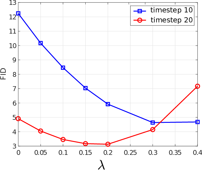
In subsection 5.1, the strengths of the extrapolations in LA-SN-DDIM were set to $\{\lambda_{i}=\lambda=0.1\}_{i=0}^{N-1}$, which led to significant performance gain for small numbers of stepsizes in comparison to SN-DDIM. We now consider how the FID scores change for different setups of $\lambda\in\{0,0.05,0.1,0.15,0.2,0.3,0.4\}$ over timesteps of 10 and 20, where $\{\lambda_{i}=\lambda\}_{i=0}^{N-1}$ for each $\lambda$ value.

Fig. 2 displays two FID curves over different $\lambda$ values, one for timestep 10 and the other for timestep 20. It is clear that for timestep 10, FID score of around 4.65 can be achieved when $\lambda=0.3$. On the other hand, for timestep 20, FID score of around 3.1 can be achieved when $\lambda=0.2$. This suggests that the setup $\lambda=0.1$ in the first experiment is far from optimality for a small number of timesteps. In other words, the FID scores in Table 1 can be improved significantly if the $\lambda$ value is tuned for different timesteps.

We note that the authors of Zhang22DEIS proposed different versions of DEIS depending on how the parameters $\{c_{ij}\}_{j=i}^{r}$ in (30) are computed. For our experiments, we used tAB-DEIS and our new method LA-tAB-DEIS. Furthermore, we also evaluated S-PNDM and LA-S-PNDM (see the update procedure of Alg. 2 in Appendix D).

The tested pre-trained models are summarized in Table 3 in Appendix E. In particular, we evaluated LA-tAB-DEIS by utilizing a pre-trained model of VPSDE for CIFAR10 in Song21SDE_gen. On the other hand, LA-S-PNDM was evaluated by utilizing four pre-trained models over four popular datasets in Liu22PNDM. The tested timesteps for each sampling method are within the range of $[10,40]$.

The performance of S-PNDM and LA-S-PNDM is summarized in the four subplots of Fig. 4, one subplot per dataset. It is seen that LA-S-PNDM outperforms S-PNDM consistently over different timesteps and across different datasets, which is consistent with the results of Table 1 in the 1st experiment. It can also be seen from the figure that the performance gain is more significant for CelebA64 and LSUN church than for CIFAR10 and LSUN bedroom. This might be because different DNN models have different fitting errors when they are being trained.

The above positive results indicate that extrapolation on the estimates of $\boldsymbol{x}$ and the high-order polynomials of the estimated Gaussian noises are compatible. In practice, one should incorporate both techniques in the sampling procedure of DPMs.

References

• (1) M. Arjovsky, S. Chintala, and L. Bottou. Wasserstein GAN. arXiv:1701.07875 [stat.ML], 2017.
• (2) K. Atkinson, W. Han, and D. E. Stewart. Numerical solution of ordinary differential equations. John Wiley & Sons, 108, 2011.
• (3) F. Bao, C. Li, J. Sun, J. Zhu, and B. Zhang. Estimating the Optimal Covariance with Imperfect Mean in Diffusion Probabilistic Models. In ICML, 2022.
• (4) F. Bao, Chongxuan Li, J. Zhu, and B. Zhang. Analytic-DPM: an Analytic Estimate of the Optimal Reverse Variance in Diffusion Probabilistic Models. In ICLR, 2022.
• (5) Christopher M. Bishop. Pattern Recognition and Machine Learning. Springer, 2006.
• (6) N. Chen, Y. Zhang, H. Zen, R. J. Weiss, M. Norouzi, and W. Chan. WaveGrad: Estimating Gradients for Waveform Generation. arXiv:2009.00713, September 2020.
• (7) P. Dhariwal and A. Nichol. Diffusion models beat gans on image synthesis. arXiv:2105.05233 [cs.LG], 2021.
• (8) I. Goodfellow, J. Pouget-Abadie, M. Mirza, B. Xu, D. Warde-Farley, S. Ozair, A. Courville, and Y. Bengio. Generative Adversarial Nets. In Proceedings of the International Conference on Neural Information Processing Systems, pages 2672–2680, 2014.
• (9) I. Gulrajani, F. Ahmed, M. Arjovsky, V. Dumoulin, and A. C. Courville. Improved training of wasserstein gans. In Advances in neural information processing systems, pages 5767–5777, 2017.
• (10) J. Ho, A. Jain, and P. Abbeel. Denoising diffusion probabilistic models. In NeurIPS, 2020.
• (11) D. P. Kingma, T. Salimans, B. Poole, and J. Ho. Variational diffusion models. arXiv: preprint arXiv:2107.00630, 2021.
• (12) M. W. Y. Lam, J. Wang, D. Su, and D. Yu. BDDM: Bilateral Denoising Diffusion Models for Fast and High-Quality Speech Synthesis. In ICLR, 2022.
• (13) L. Liu, Yi Ren, Z. Lin, and Z. Zhao. Pseudo Numerical Methods for Diffusion Models on Manifolds. In ICLR, 2022.
• (14) C. Lu, Y. Zhou, F. Bao, J. Chen, C. Li, and J. Zhu. DPM-Solver: A Fast ODE Solver for Diffusion Probabilistic Sampling in Around 10 Steps. In NeurIPS, 2022.
• (15) A. Nichol and P. Dhariwal. Improved denoising diffusion probabilistic models. arXiv preprint arXiv:2102.09672, 2021.
• (16) O. Ronneberger, P. Fischer, and T. Brox. U-Net: Convolutional Networks for Biomedical Image Segmentation. arXiv:1505.04597 [cs.CV], 2015.
• (17) J. Sohl-Dickstein, E. Weiss, N. Maheswaranathan, and S. Ganguli. Deep unsupervised learning using nonequilibrium thermodynamics. ICML, 2015.
• (18) J. Song, C. Meng, and S. Ermon. Denoising Diffusion Implicit Models. In ICLR, 2021.
• (19) Y. Song, C. Durkan, I. Murray, and S. Ermon. Maximum likelihood training of score-based diffusion models. In Advances in neural information processing systems (NeurIPS), 2021.
• (20) Y. Song and S. Ermon. Generative modeling by estimating gradients of the data distribution. In Advances in neural information processing systems (NeurIPS), page 11895–11907, 2019.
• (21) Y. Song, J. S.-Dickstein, D. P. Kingma, A. Kumar, S. Ermon, and B. Poole. Score-Based Generative Modeling Through Stochastic Differential Equations. In ICLR, 2021.
• (22) L. Yang, Z. Zhang, S. Hong, R. Xu, Y., Y. Shao, W. Zhang, M.-H. Yang, and B. Cui. Diffusion models: A comprehensive survey of methods and applications. arXiv preprint arXiv:2102.09672, 2021.
• (23) Q. Zhang and Y. Chenu. Fast Sampling of Diffusion Models with Exponential Integrator. arXiv:2204.13902 [cs.LG], 2022.
Appendix A Investigation of Computational Overhead
In addition to the evaluation of sampling qualities, we also examined the computational overhead introduced by the extrapolation operations in LA-DPMs. The minibatch size in the sampling procedure was set to 500, and the running time was measured over a windows machine with a 1080ti GPU. Table 2 displays the time complexities of different generative models over CIFAR10. It is clear from the table that the computational overhead of the extrapolation operations in LA-DPMs is negligible. This is because the extrapolation operations are linear and no additional DNN models are introduced to assist the operations.