Steering witnesses for unknown Gaussian quantum states
Abstract
We define and fully characterize the witnesses based on second moments detecting steering in Gaussian states by means of Gaussian measurements. All such tests, which arise from linear combination of variances or second moments of canonical operators, are easily implemented in experiments. We propose also a set of linear constraints fully characterizing steering witnesses when the steered party has one bosonic mode, while in the general case the constraints restrict the set of tests detecting steering. Given an unknown quantum state we implement a semidefinite program providing the appropriate steering test with respect to the number of random measurements performed. Thus, it is a ”repeat-until-success” method allowing for steering detection with less measurements than in full tomography. We study the efficiency of steering detection for two-mode squeezed vacuum states, for two-mode general unknown states, and for three-mode continuous variable GHZ states. In addition, we discuss the robustness of this method to statistical errors.
1 Introduction
The study of quantum correlations is a cornerstone of quantum information
theory enriching the foundational understanding of quantum theory and allowing
applications which outperform any classical approach in certain tasks such as
computation [1], secure communication [2] and metrology
[3].
Schrödinger [4, 5] discussed the enchanting phenomenon where one
party, Alice, is able to ”steer” the state of a distant party, Bob, by means of
entanglement they share. The implied ”action at a distance” was the core argument
in
the Einstein, Podolsky and Rosen (EPR) paper [6] against the completeness
of
quantum theory, but only lately quantum steering was conceptualized as a
particular
type of nonlocality [7].
In a quantum steering scenario two distant parties (Alice and Bob) share
a
common quantum state, where one of the parties, say Alice, is able to convince
Bob
that the state they share is entangled. She does so by performing local
measurements
and using classical communication, whereas Bob verifies whether the joint
probability distribution can be explained by a local hidden state (LHS) model
[7], in which case it rules out the possibility that Alice is steering
Bob’s
state by her choice of local measurement settings. This definition presents
quantum
steering as an intermediate form of correlation between entanglement and Bell
nonlocality. It has been intensively studied leading to some experimental
applications such as subchannel discrimination [8] and one-sided
device-independent cryptography [9].
In the context of continuous variable states [10] quantum steering
is
extensively investigated starting with Gaussian states and using Gaussian
measurements [7, 11], that have a distinct role in the
infinite-dimensional
Hilbert space, being also readily available in experiments [12, 13, 14].
In this particular case, the necessary and sufficient criterion for steerability
is
given in terms of the covariance matrix of the state [11, 15, 16], which
comprises the variances of the canonical operators. Therefore, the detection of
steering in a general unknown Gaussian state requires the full knowledge of the
covariance matrix, which might be excessive and resource-consuming.
In this paper first we prove a criterion for Gaussian steerability that
is
equivalent to known criteria in the literature, but it unfolds very nice
properties of the
covariance matrix resembling the known covariance matrix criterion of
entanglement
(see Section 3, Theorem 2). A necessary condition proof of this theorem is
presented in Ref. [15], using local uncertainty relations (LUR). Based on
this result we define
the set of linear tests detecting Gaussian steering, or witnesses, which arise
as
linear combinations of the second moments of the canonical observables. Such
tests
are commonly used for the detection of entanglement, known as entanglement
witnesses
[17, 18, 19]. An entanglement witness based on second moments is a
real
symmetric matrix such that holds for all
separable covariance matrices , while for some
entangled covariance matrix [17]. An analogous definition holds
also
for steering witnesses [20] due to the fact that the set of non-steerable
covariance matrices is convex and closed. We introduce constraints fully
characterizing the set of
Gaussian steering witnesses, which are shown to be stronger than analogous
constraints on
entanglement witnesses.
In addition, we propose a set of linear constraints that are stronger
than the constraints fully characterising the steering witnesses, however in the
particular case, when the steered party
has just one bosonic mode, these new constraints fully characterize the set of
steering
witnesses. This allows us to write a semidefinite program finding the
optimal steering test for a given state. We analyze the efficiency of steering
detection in unknown covariance matrices with respect to the number of random
measurements required for this task. For entanglement detection based on
covariance
matrices an analogous method was developed in Ref. [19], and therefore,
the
results in this article provide us with a framework of comparison between the
detection of Gaussian steering and entanglement.
The paper is organized as follows: Section 2 gives an introduction to
the
notions of Gaussian states, Gaussian measurements and symplectic transformations.
In Section 3 quantum Gaussian steering is defined and the covariance matrix
criterion for Gaussian steering is proven. In Section 4 the steering witnesses
based
on second moments are introduced and fully characterized. In Section 5 we
construct steering witnesses from random measurements acquired by homodyne
detection. Section 6 presents the results of steering detection in two-mode
squeezed vacuum
states and in two-mode general unknown states. Also, we illustrate the example of
steering detection in three-mode continuous variable GHZ states, where the
steered party has two modes. In Section 7 the statistical analysis of
our method is provided. The summary and conclusions are expanded in Section 8.
2 Gaussian states
A continuous variable (CV) system of bosonic modes is described by the canonical operators of position and momentum and in the Hilbert space , where is the infinite-dimentional Hilbert space of mode [10, 12, 13]. Defining the vector of canonical operators one obtains the commutation relation written as (we assume ):
| (1) |
where is the identity matrix, and are the elements of the symplectic matrix
| (2) |
Gaussian states are fully described by the first and second order statistical moments, namely the displacement vector , and the covariance matrix (CM) with its elements defined as [14, 21]:
| (3) |
where represents the anticommutator. The CM of a physical quantum state has to fulfill the Robertson-Schrödinger uncertainty relation, which we will often refer to as covariance matrix criterion (CMC):
| (4) |
In the following we will mostly consider a bipartite Gaussian quantum state of modes with the CM of the following block structure:
| (5) |
where and are the CMs of the subsystems of Alice and Bob with and modes, respectively, is the correlation matrix between the two parties, and . It can be readily shown that the uncertainty relation in Eq. (4) directly implies , and .
A much more general approach in describing any mode CV state is based on the completeness of the set of displacement operators in phase space defined as:
| (6) |
where is a real vector of phase space variables. The connection between Hilbert space and phase space descriptions is given by the Fourier-Weyl relation for a given density operator in Hilbert space [10]:
| (7) |
from where the characteristic function is readily defined as . If represents a Gaussian state then its characteristic function takes a particular form [10]:
| (8) |
where the first moments are considered to be zero and is the CM
associated with the Gaussian density operator . A Gaussian measurement
[22] applied on Alice’s subsystem can be described by a positive Gaussian
operator with a CM given by satisfying the CMC: . The calculation of , where is the identity operator defined on
Bob’s space, transforms into a multivariate Gaussian integral on characteristic
function level. The remaining modes of Bob’s conditioned state
after measurement form a Gaussian state with CM given by
, which
represents the Schur complement of the matrix with
respect to the submatrix [10]. The following Lemma of the
Schur
complement will be useful in further discussions on Gaussian steering.
Lemma 1 [23]. Consider a Hermitian matrix
| (9) |
Then if and only if and , where is the
Schur complement of block of the matrix .
Given that is a CM satisfying the uncertainty relation in Eq. (4) we have and , and hence the Schur complement of with respect to is also a positive matrix . Let us consider the matrix , with , and its Schur complement with respect to . Applying the positivity conditions from Lemma 1 leads to the Schur complement [10, 24]
| (10) |
which means that the matrix set on the right-hand side has a supremum (i.e. a minimum upper bound) with respect to the Löwner partial order ( if and only if is positive semidefinite), and that this supremum is given by the Schur complement on the left-hand side.
2.1 Symplectic transformations
The equivalent of unitary operators acting on the quantum state space are the symplectic transformations on CMs, which are symmetric real matrices acting by congruence on CMs: . The singular value decomposition of a real symplectic matrix gives [25]:
| (11) |
where is a one-mode squeezing matrix (symplectic and nonorthogonal) with the squeezing parameter:
| (12) |
and , are symplectic and orthogonal matrices. Denote by the group of orthogonal symplectic matrices isomorphic to the group of complex unitary matrices [25]:
| (13) |
where the corresponding symplectic matrices are given by:
| (14) |
According to the Williamson theorem [27] every real symmetric matrix can be brought to a diagonal form through symplectic transformations as follows:
| (15) |
where are called symplectic eigenvalues of . By
| (16) |
we denote the symplectic trace of the matrix .
3 Gaussian quantum steering
Consider the situation where Alice and Bob are two distant parties sharing a common state , and Alice performs local measurements on her state, with eigenvalues . A formal definition of steering says that Alice is not able to steer Bob’s state if there exists an ensemble of preexisting local hidden states with probabilities , and a stochastic map 11 1 denotes the probability distribution of Alice to obtain outcome when measuring and given a local hidden variable . from the hidden variable to , such that Bob’s conditioned state after Alice’s measurement is given by [7]:
| (17) |
This represents the local hidden state (LHS) model, where Bob checks if Alice can
simulate the state based on her knowledge of the parameter
, by drawing the states according to the distribution .
Conversely, if Bob cannot find any ensemble and map
satisfying Eq. (17), then Bob must admit that Alice can steer his
system.
In the Gaussian realm where the joint state is a Gaussian
state
with CM , we consider that Alice’s measurement is also Gaussian
(i.e.
mapping Gaussian states into Gaussian states). As discussed in the previous
section a
Gaussian measurement is represented by a positive operator with a
Gaussian
characteristic function as in Eq. (8) with CM , satisfying
. When Alice performs a measurement and gets an
outcome , Bob’s conditioned state is a Gaussian state with
CM
given by
[10]. In Ref. [7] a criterion for Gaussian steerability of CM
was derived:
Theorem 1. [7] A Gaussian state with covariance matrix with the block form defined in Eq. (5) is Alice Bob non-steerable by Gaussian measurements if and only if
| (18) |
or, equivalently22 2 This follows from applying the positivity conditions from Lemma 1 to the total matrix in Eq. (18).
| (19) |
holds, where is the Schur complement of with respect to submatrix
and is the symplectic matrix of modes as defined
in
Eq. (2).
From the previous section we know that the Schur complement of a CM is a positive
matrix.
However, for a non-steerable Alice to Bob Gaussian state the Schur complement of
its CM
with respect to has to satisfy a stronger condition than positivity,
namely the CMC from Eq. (4). An important result of this article is given
by
the following theorem on Gaussian non-steerability.
Theorem 2. A bipartite quantum Gaussian state with covariance matrix with blocks defined in Eq. (5) is Alice Bob non-steerable by means of Gaussian measurements if and only if there exists a covariance matrix corresponding to Bob’s system satisfying , such that:
| (20) |
Proof.
Theorem 1 states that the Schur complement
of a
non-steerable CM is also a CM, i.e.
. Based also on the definition
of the Schur
complement in Eq. (10) we state that if a CM is
non-steerable
then there exists a CM fulfilling Eq. (20), and it is the Schur
complement .
Conversely, if the relation in Eq. (20) is fulfilled for
some CM , satisfying CMC , then by
the definition of the Schur complement in Eq. (10) it follows
that there exists a positive semi-definite matrix such that:
. Therefore, the Schur complement
also has to fulfill the CMC, since , which based on Theorem 1, means that
is a non-steerable quantum state.
∎
In Ref. [15] a one way proof of this theorem based on local uncertainty relations (LURs) is provided. The non-steerability criterion formulated in Theorem 2 shows a strong similarity to the separability of Gaussian states. A continuous variable state with CM is separable with respect to parties if and only if there exist local CMs and for each partition, such that [26]. Hence, it is obvious that any separable Gaussian state is also non-steerable by Gaussian measurements since holds. Thus, Gaussian non-steerability represents a stronger condition than separability of Gaussian states.
4 Steering witnesses based on second moments
Based on Theorem 2 we can define the set of non-steerable CMs as follows:
| (21) |
where denotes Alice to Bob non-steerability, and is a positive-semidefinite matrix. The set of non-steerable CMs by Gaussian measurements forms a closed convex subset of the space of all covariance matrices, similarly to the set of all CMs and the set of separable CMs. This allows to completely describe the set of non-steerable CMs by a family of linear inequalities representing the steering witnesses (SWs).
Definition 1. We define the set of real symmetric -matrices
| (22) |
where is the CM of a bipartite system with modes,
denotes Alice to Bob non-steerability, where is defined in Eq.(21). All matrices
for which there exists
with will
be called steering witnesses (SWs).
This Definition 1 is very similar to the Definition 6.4 in Ref. [18] for
entanglement witnesses (EWs) since it relies solely on the fact that the set of
non-steerable CMs and the set of separable CMs are both convex and closed sets.
There it is also shown that for any such hyperplane holds, which
follows from the positivity of CMs. We proceed, in analogy with the methods used
in Ref. [18], to characterise the set of SWs and prove some of their
properties.
Theorem 3. Let be a real symmetric matrix on a phase space of modes, with and denoting the block diagonal submatrices of corresponding to subsystems of Alice and Bob, respectively. Then is a steering witness, namely , if and only if
| (23) | ||||
| (24) | ||||
| (25) |
Proof.
Below Theorem 6.2 in Ref. [18] it is proven that any
hyperplane cutting the set of CMs is represented by a positive semi-definite
matrix,
and therefore, condition holds for any EW and SW as well. In addition,
in
Theorem 6.3 in the same reference it is proven that such a test represented by
and satisfying also is equivalent to obtaining
for all CMs . In the following we will prove
that
condition guarantees that for all non-steerable CMs. Therefore,
condition
together with conditions (23, 24)
assure that there exists a CM such that , i.e. it
is steerable.
Consider the SWs based on second moments of the following block form:
| (26) |
In the following we will use an important result discussed in Ref. [18] 33 3 The expression represents the value of the ground state energy of the Hamiltonian defined as , where is the vector of canonical operators.:
| (27) |
where the minimization is performed over the set of CMs .
We have to prove that condition in Eq.(24) holds for any
SW
described in Definition 1 (22). Based on Theorem 2 for any
there exists a CM
corresponding to the quantum state of Bob such that:
| (28) |
holds. Moreover, the matrix is a non-steerable CM itself, and from the Definition 1 of SWs in Eq. (22) we have the following condition:
| (29) |
Using Eq. (27) we conclude that SWs have to fulfill the condition
| (30) |
Conversely, we prove that a matrix satisfying the conditions in Eq. (24) represents a SW with for any non-steerable CM . Starting from Eq. (24) and using Eq. (27) we have that
| (31) |
holds for any valid CM . Now, any non-steerable CM fulfills (Theorem 2) such that the condition holds. Therefore we get for any non-steerable state . ∎
We are now in the position to summarize the results for the detection of Gaussian
steering with witnesses based on second moments.
Theorem 4. [Steerability] A CM of two parties consisting of modes is Alice to Bob steerable by means of Gaussian measurements if and only if there exists a such that:
| (32) |
where is a real symmetric matrix satisfying
| (33) |
where denotes the principal submatrix of belonging to the subsystem of
Bob. Matrices are called steering witnesses based on second moments.
The EWs defined in Refs. [17, 18] that detect bipartite entanglement fulfill the condition , where denote the two parties, and are the block diagonal matrices of the EW associated with each party. SWs are characterised by stronger constraints than these and therefore, any SW based on second moments is also an EW. This is consistent with the fact that any steerable state necessarily contains also entanglement.
5 Linear constraints for steering witnesses
In the following we present linear conditions for the SWs that are
stronger than Eq. (33) in Theorem 4, such that the SWs can be
calculated by a semidefinite program (SDP) to detect
steering in a given CM. An analogous idea for EWs was developed in Ref.
[19].
Proposition 1. For the steering witness of an mode covariance matrix steerable from Alice to Bob, with , the inequalities (33) are satisfied if (if and only if for ) the following conditions are fulfilled:
| (34) |
Proof.
Since is a positive semidefinite matrix, also the principal submatrix is positive semidefinite. For every such matrix there exists a symplectic transformation that brings it to its Williamson normal form as follows 44 4 Given that holds for any positive matrix [28], the symplectic transformations do not only preserve the symplectic eigenvalues, but also positivity.:
| (35) |
with , where , are positive symplectic eigenvalues of . By imposing the positivity condition on the eigenvalues of the total matrix in Eq. (35) we arrive at the following inequality for the symplectic eigenvalues:
| (36) |
Now, the sum of symplectic eigenvalues gives:
| (37) |
∎
Relation (36) explains why the conditions on SWs given in the Proposition 1 are stronger than Eq. (33) from Theorem 4: it imposes a lower bound on the symplectic eigenvalues that is strictly greater than zero, as . This assures that the sum of symplectic eigenvalues exceeds , however, it rules out the possibility that some symplectic eigenvalues may satisfy . An exception represents the case when the steered party has one mode (=1) and in Eq. (5) is a matrix with only one symplectic eigenvalue satisfying , which is equivalent to relation (33). However, the interval of forbidden symplectic eigenvalues is the largest for , while in the limit of large we have , and the constraints in Proposition 1 become equivalent to the constraints fully characterizing SWs in Theorem 4.
5.1 Constructing witnesses
We are now able to define an SDP by constructing the witnesses from given (random) measurements using the linear constraints in the Proposition 1. Given the repeated independent measurements on the CM, the witness operator is represented by , where the coefficients are the output of the optimization algorithm. According to the Proposition we can detect the Gaussian steering from Alice to Bob in two-mode CMs with the following SDP:
| (38) | ||||||
where is the vector of coefficients and , with being the vector of measurement matrices , which represent the homodyne detection measurements as constructed in Ref. [19].
Consider an experimental scheme detecting two-mode CMs using a single homodyne detector, a phase shifter of angle between the vertical and horizontal polarization components, a polarization rotator on angle and a polarizing beam splitter, for mixing the initial modes denoted by and [29]. The mode arriving at the detector has the following expression:
| (39) |
The generalized quadrature operator is given by:
| (40) |
which covers the whole continuum of quadratures in terms of initial modes and for , and . With homodyne detection one can measure the statistical moments of the quadrature up to the second order [29], and therefore, one can readily calculate the variance of the quadrature as follows:
| (41) |
where is the measurement matrix of the variances we use in Eq. (38):
| (42) |
The mode CM is a symmetric, real matrix with independent parameters. Therefore, for the CM reconstruction of a two-mode Gaussian state one needs distinct measurement directions given by the angles , and . This scheme can be extended to modes with a single homodyne detector by using the same two-mode combination scheme times. Starting with three initial modes , and , the generalized mode arriving at the detector would be:
| (43) |
6 Detection of Gaussian steering
Our method of detection relies on the SDP described in Eq. (38), where we
run the optimisation starting with two measurement settings, and then adding
other
measurements, one by one, until steering is detected. In this way we are able
to evaluate the efficiency of steering detection in terms of the number of
required
measurement settings. In the case of general quantum states of
unknown origin the best strategy could be to perform random measurements, which
in
our case reduces to choosing random values for angles , and
.
A measure for quantifying steering of a bipartite Gaussian
state with CM defined in Eq. (5) was proposed in Ref.
[11]. In particular, the
nonsteerability condition in Eq. (19) is equivalent to
for all , where represent the symplectic
eigenvalues
of the Schur complement . The Gaussian
steerability can then be quantified via [11]:
| (44) |
This expression is invariant under local symplectic transformations at the CM level, and has a formal similarity to the logarithmic negativity [30], which for Gaussian states quantifies how much the partially transposed CM fails to fulfill CMC in Eq. (20). The quantification of Gaussian steerability takes a simpler form when the steered party, e.g. Bob, has one mode only [11]:
| (45) |
Steering can also be quantified by a minimal SW, where corresponds to the smallest possible value for a CM . The program proposed in Eq. (38) may reach the minimal value with more measurements than in full tomography, since the linear constraints used in the optimization for finding the appropriate SWs are stronger than required in Theorem 4. For two-mode CMs our method shows that the minimal SW is related to the steerability measure from Ref. [11] as follows:
| (46) |
6.1 Two-mode squeezed vacuum states
First we test our method on the class of two-mode squeezed vacuum states (SVS), which are easily accessible in experiments [14]. The CM is of the following form:
| (47) |
where is the squeezing parameter. For this particular case, using formula (45), the expression quantifying steering is a monotonic function in :
| (48) |
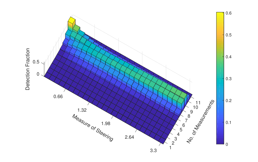
In Fig. 1 we show the fraction of SVS certified with steering with respect to the number of measurements performed randomly. First, we notice the similarity between the detection of SVS with higher steering and the detection of high entanglement [19], since both require measurements on average. However, SVS with less entanglement can be certified in many cases with measurements, on the other side the detection of low steering mostly requires measurements (full tomography). The demand on more measurements for steering detection in comparison with entanglement is consistent with the fact that SWs based on second moments satisfy stronger constraints than EWs (see discussion below Theorem 4).
6.2 Random two-mode covariance matrices
For the case of general unknown CMs we test our method by generating random two-mode CMs and using random measurements. We start with a CM of a thermal state, which is a diagonal matrix with the symplectic eigenvalues for every mode , related to the thermal photon number as [14]:
| (49) |
where are randomly generated from a uniform distribution in a finite interval , . Any general CM can be obtained from a thermal state CM that undergoes a symplectic transformation:
| (50) |
For random symplectic matrices we use the singular value decomposition (see Eq (11)). We randomly generate unitary matrices and from the Haar distribution, while for one-mode squeezers we create random parameters by a uniform distribution in a finite interval. The MATLAB code generating symplectic matrices as described above, was developed in Ref. [31].

In Figure 2 we illustrate the data from running the algorithm for different randomly generated CMs of thermal states with symplectic eigenvalues randomly generated from a finite interval and symplectic eigenvalues with squeezing parameters . It shows the efficiency of steering detection by calculating the SW (see Eq. (38)) for every newly added measurement direction until it finds steering. Comparing to the particular case of SVS discussed in Figure 1 the detection of steering in general CMs shows slight improvement for low steering where only for a fraction of of the CMs steering was certified by the 10th measurement. For high steering one may need most of the time measurements for the detection of steering. The detection of two-mode Gaussian steering shows a similar behaviour as the detection of entanglement in randomly generated CMs [19]. The stronger the correlation the easier steering or entanglement can be detected ( i.e. it requires fewer measurements).
6.3 Three-mode continuous variable GHZ states
The CV counterpart for the GHZ three qubit states is experimentally created from three squeezed beams (two position-squeezed beams with squeezing and one momentum-squeezed beam with squeezing ) which are mixed in a double beam splitter [32]. The CM obtained in this manner corresponds to a pure, symmetric, genuine multipartite entangled three-mode Gaussian state, also known as CV GHZ state [33]:
| (51) |
where is related to the squeezing parameters in momentum and position as [33]:
| (52) |
and
| (53) | ||||
| (54) |
In fact, a proper (unnormalized) CV GHZ state is a simultaneous eigenstate with zero eigenvalues of total momentum and relative positions , whereas the CV state described in Eq. (51) approaches the CV GHZ state in the limit of infinite squeezing [34].

Let us consider the partition where Alice has one mode (it is not
important which mode, due to the special form of the CM in Eq. (51)) and
Bob has the other two modes. By calculating the symplectic eigenvalues of the
Schur complement corresponding to the situation where Alice is trying to steer
Bob’s state by her choice of measurements (see Theorem 1), we obtain that the CV
GHZ state is steerable for , and the amount of steering is given by the
measure in Eq. (44).
In Figure 3 we present the efficiency of steering detection in GHZ
states described by the CM given in Eq. (51) using the method of SWs as a
function of the number of random measurements. The algorithm was applied to
samples, where for each sample the number of measurement
settings to detect steering was recorded. For three-mode CMs there are
independent measurement settings required for full tomography, whereas with our
method we detect steering mostly with measurements. This is despite the fact
that in our case , and the linear constraints for the SWs defined in
Proposition 1 are stronger than required in Theorem 3. However, a small fraction
of of steerable GHZ states are detected by more measurements than needed in
full tomography.
7 Statistical analysis
In real experiments the homodyne data is obtained by repetitions of a measurement with direction , giving rise to a collection of outcomes , (). In the case of Gaussian states these outcomes are governed by the normal probability distribution with the mean , and variance (see Sec. 5). The variances are estimated by the sample variances, which follow the distribution [35]. From the statistical error carried out by a distribution and using standard error propagation the resulting error for becomes [19]:
| (55) |
Our method of steering detection is based on the SDP presented in Section
5
where the coefficients are calculated using as input data. However,
the
formula in Eq. (55) does not take into account that these two variables
are
not independent. We overcome this difficulty by using two sets of homodyne data,
from the first one we derive the coefficients and the second one is used to
evaluate and [36].
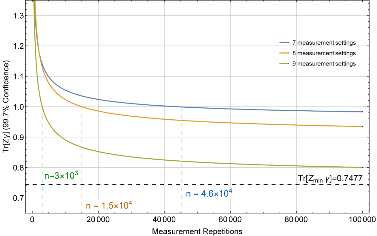
In Figure 4 we show the estimated value of the SW with the confidence for a steerable squeezed vacuum state CM with , as a
function of measurement repetitions . We can see that detecting steering with
measurement settings would require much more repetitions of the
measurements compared
to the case of measurement settings. As a result, the total number of
measurements is
one order of magnitude less for measurement settings ()
than in the case of different measurement settings (). Therefore, statistical analysis may help the experimentalist to decide
whether it is more advantageous to add new measurement directions or to increase
the number of repetitions of the measurements in order to detect
steering.
8 Summary and conclusions
Non-steerable Gaussian states have covariance matrices (CMs) forming a closed and convex set, which gives rise to hyperplanes or steering witnesses (SWs) , separating any other point from this set. This is easily seen from Theorem 2 which provides a criterion for non-steerable CMs. Based on this result we characterized the SWs for Gaussian states by providing a set of constraints to be satisfied by any such witness.
The method of detecting quantum correlation by witnesses has proven to be very useful and accessible in experiments with entangled states [37], while an extensive study about the efficiency of entanglement detection with random measurements in continuous variable states was presented in Ref. [19]. In this article we have developed similar optimization tools for detecting steering in Gaussian states with similar complexity and scaling behaviour.
We proposed a set of stronger linear constraints on steering witness operators in comparison to entanglement witnesses (EWs) and studied the efficiency of steering detection with respect to the number of measurement settings. These linear constraints are proven to fully characterize the set of steering witnesses when the steered party has only one bosonic mode. The SDP we developed in Section 5 uses random measurements of variances from the homodyne detection, as the building blocks for constructing the optimal steering test for a given unknown state.
In the case of two-mode squeezed vacuum states we noticed that detection of steering in Gaussian states requires more measurements on average than for entanglement detection [19]. This lies in agreement with the fact that SWs satisfy stronger conditions than EWs (see the discussion above Theorem 4).
We applied our method also for general random two-mode Gaussian states. In this
case, the
detection of both types of quantum correlations, i. e. entanglement and
steering,
has a behaviour confirming the general idea that higher quantum correlations are
easier to detect. In particular, high steering and entanglement in two-mode
states
are typically detected by measurement settings using our method, while
full
tomography requires measurement settings.
In addition, we provided an example of steering detection when the
steered party consists of more than one mode, namely the three-mode continuous
variable GHZ states. In this case the linear constraints used in the optimization
are stronger compared to the SW constraints in Theorem 4, reducing the set of
possible SWs. Nevertheless, the result shows that in most of the cases the GHZ
states are detected with steering by measurements or less, which is two
measurements fewer than in full tomography. For -mode CMs when the steered
party (Bob) has number of modes we have shown that the
linear constraints tend to be equivalent to the exact constraints fully
characterizing the set of SWs. Therefore, our method of steering detection may
become better for larger number of modes. We provided also a statistical analysis
of our
method showing a good robustness to statistical errors.
Acknowledgements.
D.B. and H.K. acknowledge financial support by the QuantERA project QuICHE via the German Ministry of Education and Research (BMBF Grant No. 16KIS1119K) and by the Deutsche Forschungsgemeinschaft (DFG, German Research Foundation) under Germany’s Excellence Strategy - Cluster of Excellence Matter and Light for Quantum Computing (ML4Q) EXC 2004/1 - 390534769. T.M. and A.I. acknowledge financial support received from the Romanian Ministry of Research, Innovation and Digitization, through the Project PN 23 21 01 01/2023.
References
References
- [1] D. Bruß, G. Leuchs, Eds., Quantum Information: From Foundations to Quantum Technology Applications, 2nd Edition, Wiley-VCH (2019)
- [2] F. Grasselli, G. Murta, H. Kampermann, D. Bruß, Entropy Bounds for Multiparty Device-Independent Cryptography, PRX Quantum 2, 010308 (2021)
- [3] E. Polino, M. Valeri, N. Spagnolo, and F. Sciarrino, Photonic quantum metrology, AVS Quantum Sci. 2, 024703 (2020)
- [4] E. Schrödinger, Discussion of Probability Relations between Separated Systems, Proc. Cambridge Philos. Soc. 31, 555 (1935)
- [5] E. Schrödinger, Probability relations between separated systems, Proc. Cambridge Philos. Soc. 32, 446 (1936)
- [6] A. Einstein, B. Podolsky, N. Rosen, Can Quantum-Mechanical Description of Physical Reality Be Considered Complete?, Phys. Rev. 47, 777 (1935)
- [7] S. J. Jones, H. M. Wiseman, A. C. Doherty, Entanglement, Einstein-Podolsky-Rosen correlations, Bell nonlocality, and steering, Phys. Rev. A 76, 052116 (2007)
- [8] M. Piani, J. Watrous, Necessary and Sufficient Quantum Information Characterization of Einstein-Podolsky-Rosen Steering, Phys. Rev. Lett. 114, 060404 (2015)
- [9] C. Branciard, E. G. Cavalcanti, S. P. Walborn, V. Scarani, H. Wiseman, One-sided device-independent quantum key distribution: Security, feasibility, and the connection with steering, Phys. Rev. A 85, 010301(R) (2012)
- [10] A. Serafini, Quantum continuous variables: A primer of theoretical methods, Taylor & Francis Group (2017)
- [11] I. Kogias, A. R. Lee, S. Ragy, G. Adesso, Quantification of Gaussian Quantum Steering, Phys. Rev. Lett. 114, 060403 (2015)
- [12] S. Olivares, Quantum optics in the phase space, Eur. Phys. J. Spec. Top. 203, 3 (2012)
- [13] A. Ferraro, S. Olivares, M. G. A. Paris, Gaussian states in continuous variable quantum information, Bibliopolis, Napoli (2005)
- [14] C. Weedbrook, S. Pirandola, R. Garcia-Parton, N. L. Cerf, T. C. Ralph, J. H. Shapiro, S. Lloyd, Gaussian quantum information, Rev. Mod. Phys. 84, 621 (2012)
- [15] S.-W. Ji, J. Lee, J. Park, H. Nha, Steering criteria via covariance matrices of local observables in arbitrary-dimensional quantum systems, Phys. Rev. A 92, 062130 (2015)
- [16] M. Frigerio, C. Destri, S. Olivares, M. G. A. Paris, Quantum steering with Gaussian states: A tutorial, Phys. Lett. A 430, 127954 (2022)
- [17] P. Hyllus, J. Eisert, Optimal entanglement witnesses for continuous-variable system, New J. Phys. 8, 51 (2006)
- [18] J. Anders, Estimating the degree of entanglement of unknown Gaussian states, Diploma Thesis, University of Potsdam (2003), arxiv:quant-ph/0610263
- [19] T. Mihaescu, H. Kampermann, G. Gianfelici, A. Isar, D. Bruss, Detecting entanglement of unknown continuous variable states with random measurements, New J. Phys. 22, 123041 (2020)
- [20] R. Ma, T. Yan, D. Wu, X. Qi, Steering witnesses and steering criterion of Gaussian states, Entropy 24, 62 (2022)
- [21] R. Simon, N. Mukunda, B. Dutta, Quantum-noise matrix for multimode systems: invariance, squeezing, and normal forms, Phys. Rev A 49, 1567 (1994)
- [22] J. Fiurášek, Gaussian Transformations and Distillation of Entangled Gaussian States, Phys. Rev. Lett. 89, 137904 (2002)
- [23] F. Zhang, The Schur complement and its applications, Springer (2005)
- [24] L. Lami, A. Serafini, G. Adesso, Gaussian entanglement revisited, New J. Phys. 20, 023030 (2018)
- [25] A. B. Dutta, N. Mukunda, R. Simon, The real symplectic groups in quantum mechanics and optics, Pramana-J. Phys. 45, 471 (1995)
- [26] R. F. Werner, M. M. Wolf, Bound entangled Gaussian states, Phys. Rev. Lett. 86, 3658 (2001)
- [27] J. Williamson, On the algebraic problem concerning the normal forms of linear dynamical systems, Amer. J. Math. 58, 141 (1936)
- [28] R. Bhatia, T. Jain, On symplectic eigenvalues of positive definite matrices, J. Math. Phys. 56, 112201 (2015)
- [29] V. D’Auria, A. Porzio, S. Solimeno, S. Olivares, M. G. A. Paris, Characterization of bipartite states using a single homodyne detector, J. Opt. B.: Quantum Semiclass. Opt. 7, S750 (2005)
- [30] Plenio, M. B., Logarithmic Negativity: A Full Entanglement Monotone That is not Convex, Phys. Rev. Lett. 95, 119902 (2005)
- [31] D. P. Jagger, MATLAB toolbox for classical matrix groups, M. Sc. Thesis, University of Manchester (2003)
- [32] P. van Loock, S. L. Braunstein, Multipartite Entanglement for Continuous Variables: A Quantum Teleportation Network, Phys. Rev. Lett. 84, 3482 (2000)
- [33] G. Adesso, A. Serafini, F. Illuminati, Three-mode Gaussian states in quantum information with continuous variables, https://doi.org/10.48550/arXiv.quant-ph/0609071 (2006)
- [34] P. van Loock, S. L. Braunstein, Greenberger-Horne-Zeilinger nonlocality in phase space, Phys. Rev. A 63, 022106 (2001)
- [35] K. Knight, Mathematical Statistics, Chapman and Hall, New York (2000)
- [36] T. Moroder, M. Kleinmann, P. Schindler, T. Monz, O. Gühne, R. Blatt, Certifying experimental errors in quantum experiments, Phys. Rev. Lett. 110, 180401 (2013)
- [37] O. Gühne, G. Toth, Entanglement detection, Phys. Rep. 474, 1 (2009)