Improving Composition of Ultra High Energy Cosmic Rays with Ground Detector Data
Abstract
We show that the maximum shower depth () distributions of Ultra-High Energy Cosmic Rays (UHECRs), as measured by fluorescence telescopes, can be augmented by building a mapping to observables collected by surface detectors. The resulting statistical improvement of such augmented dataset depends in a universal way on the strength of the correlation exhibited by the mapping. Building upon the publicly available data on “golden hybrid” events from the Pierre Auger Observatory we project possible improvements in the inferred composition of UHECRs for a range of possible mappings with varying correlation strengths.
I Introduction
Cosmic rays (CRs) with ultra-high energy, eV, are studied through the observation of the Extensive Air Showers (EAS) that are generated in the Earth atmosphere. The Pierre Auger Observatory PierreAuger:2015eyc employs a “hybrid” detection method: Surface Detectors (SD) measure electrons and muons propagating to the surface, while Fluorescent Detectors (FD) capture the isotropic light emitted by excited nytrogen and can track the development of the EAS. In particular, the former can measure the atmospheric depth at which the number of charged particles is at its maximum, , which is in turn a key ingredient to infer the mass composition of CRs.
While the hybrid measurement technique provides detailed insights for the EAS study, the runtime of FDs is largely limited by background light noise. This results in of the total number of showers observed to be reconstructed as “hybrid”, i.e. with both FD and SD data, while the remaining part of the dataset is measured with the SD only. For example, in the Pierre Auger 2021 Open Data the_pierre_auger_collaboration_2021_4487613, there are 22731 SD measurements of EAS, which we refer to as Non-Hybrid (NH) showers, and 3156 “brass hybrid” (BH) events, that is showers that have been recorded simultaneously by the SD and the FD. Of these BH, 1602 are called “golden hybrids” (GH), with independent SD and FD reconstructions. The low statistics of BH and especially GH events compared to NH is currently a dominant limiting factor in the determination of the CR mass composition.
A possible solution is to infer from ground data, exploiting GH events to build a map between SD and FD observables. Unfortunately, linear and simple non-linear fits based solely on measured data, such as the variable proposed in Ref. PierreAuger:2017tlx, exhibit only relatively low levels of predictive power. Recently, an alternative has been proposed in terms of a Deep Neural Network trained on simulated ground data for 4 different primaries to directly predict PierreAuger:2021fkf. Unfortunately, simulations currently cannot faithfully reproduce the observed ground data of Pierre Auger events Cazon:2020zhx. This exposes any approach directly relying on such simulations to potentially large systematic errors. In addition, the chosen composition of simulated events used to train the network can act as a confounding variable on the inferred . This can in turn lead to biased estimates of CR composition.
In this work we address these drawbacks and propose a general method to exploit any observed correlations between SD and FD data, to effectively increase the statistics of . After briefly reviewing possible maps in Section II, in Section III we show a rigorous way to combine the GH data with the inferred one, which leads to the enhancement of the dataset by an effective number of GH showers, . The latter number monotonically increases with the level of correlation given by the map. Finally, in Section IV we employ this method to improve the results on the full mass composition obtained in Ref. Bortolato:2022ocs.
II Correlating ground detector data with
For our purpose the -th GH event in the dataset can be characterized by one FD measurement, , and a set of SD observables, . We can then consider functions of SD observables for which the GH set exhibits some correlation between and , as parametrized by
| (1) |
where , and are the standard deviations of and and their covariance, respectively.
Possibly the simplest example of is the weighted average of
| (2) |
where the weights are fixed by maximizing . For simplicity, we assume that the PDF of each variable is a normal distribution described by its measurement and the respective uncertainty. Namely, we have
| (3) |
and similarly for . Note that the fit has to be performed separately for each subset of GH events (i.e. in a particular CR energy bin or angular window) for which one wants to infer composition. This ensures an unbiased estimator, assuming the GH and NH events in the same subset are of the same composition and follow the same distribution of .
As a proof of concept, we use the set of observables11 1 We have repeated this exercise with multiple combinations of available observables. The chosen set represents the one with the largest correlation achievable without overfitting of the data.
| (4) |
with their respective uncertainties. Here, is the azimuthal angle of the shower core, while is the duration of the signal in the -th Cherenkov station hit by the shower, defined as the difference between the final and initial time bin. We take the mean, standard deviation and maximum values over the active stations for each event. For each shower, we generate multiple samples of the observables from their PDF, eq. (3). In such a way, we can also compute the uncertainty associated with . Uncertainties on the bins and are not provided in the Open Data, hence we assume the uncertainties on both quantities to be one bin. These samples are then utilized to maximize through the “Nelder-Mead” method (any similar optimization algorithm would work). Finally, we employ -folding to check for overfitting. Following this procedure, we are able to achieve correlation between and for GH in the energy bin EeV, with 455 GH showers. We chose this bin as the only one where GH and NH data overlap in the Pierre Auger Open Data set.
In practice, more advanced approaches, such as non-linear fits or neural networks, may be employed to obtain stronger correlations between and . As two explicit examples of such more complicated observables, we mention the variable PierreAuger:2017tlx and the Deep Neural Network trained on simulated ground data PierreAuger:2021fkf. In the same energy bin, the former yields 22 2 Uncertainties due to limited statistics and above stated systematics in both cases have been estimated using bootstrapping EfroTibs93., while the latter can reach . We stress that for our purpose the strength of an observable is measured solely in terms its correlation with as established on a particular measured GH dataset . In this way we avoid potential systematic biases associated with direct inference of individual from non-equivalent datasets or simulations.
III Inference of distribution
Following the previous Section, we can represent the GH dataset as a set of pairs , with , and we assume that there is some level of correlation between the two observables. The NH dataset is then represented by the pairs , with , where . In the latter set the entries, which are missing in the original data, can be inferred by exploiting the map built through the set correlation, that is .
Let be the joint probability distribution of the set. For simplicity, we start by assuming that such distribution follows a Bivariate Normal (BN) model, while we comment later for the general case. Each BN distribution is defined by the means , , the standard deviations , and the correlation . The conditional distribution is then simply given by the normal distribution with mean and standard deviation . Therefore one can sample following the formula
| (5) |
where accounts for systematic uncertainty of , and is a random number drawn from a normal distribution, . In this way we obtain a set of inferred values, .
Due to the finite number ( and ) of events, we need to account for statistical uncertainties in the inference via bootstrapping EfroTibs93. The latter method consists of inferring values for each multiple times, each time starting with a different set of pairs , called the bootstrapped sample. The procedure is repeated times, where each time the bootstrapped sample is given by sampling pairs from the first set with allowed repetitions.
Namely, at bootstrap step , where , we have
| (6) |
Here and represent the systematic uncertainties on and , while . Finally, the dimensional vector is drawn from the Multinomial distribution with events and classes which are all equally probable, . The values in this array, , count how many times each pair is chosen in the -th bootstrapped sample. It thus satisfies the relation . As a result of this procedure, we obtain at each step the set of couples
| (7) |
We can now estimate the -th joint distribution from the bootstrapped samples.
Similarly, we define
| (8) |
where now the index runs over the elements, , and . The account for both statistical and systematic uncertainties.
For each bootstrapped sample we can now obtain a set of pairs
| (9) |
where the first component of the pair is inferred by plugging in Eq. (5). Finally, we can combine the two sets to obtain
| (10) |
At this point, one can use the larger combined dataset to perform the desired analysis. As we obtain the elements from the inference method described above, it is fair to ask what is the gain in terms of statistical power with the combined dataset. In order to estimate it, we can compute the variance of the distribution of the means, . That is, we compute the mean value of for each set, ; the resulting distribution defined by all is a Gaussian with variance . The ratio between the variances obtained with the initial dataset and with the combined one, , can provide a measure of the improvement in the statistical significance obtain with this method. Indeed, the quantity
| (11) |
can be interpreted as the effective increase of events in the combined dataset, with respect to the original one, . This interpretation follows from the fact that the variance of the mean distribution is given by the variance divided by the number of events. Namely, if it means no additional information is contained in the inferred set . On the contrary, if the effective statistical power of amounts to have total events. The functional dependence of on the correlation , for different values of and , is shown in Figs. 1 and 2. Points in these figures are obtained numerically, with the procedure described above, using bootstrapped samples. Furthermore, we assumed that systematic uncertainties are small. The latter translates to have in Eq. (5). In this scenario, the ratio increases monotonically with and does not depend on the number of events and , but only on their ratio, see Fig. 1. Larger ratios allow then for larger values of for the same level of correlation, as shown in Fig. 2.
In the limit of , tends to the maximal value . In practice, cannot be obtained with a finite number of events due to statistical uncertainties, thus the maximum value of is smaller.
In the general case, the joint distribution does not follow a BN distribution. One may then try to use Kernel Density Estimation (KDE) to obtain ; however, if the latter is computed inappropriately, we may introduce a bias in inferring values (variance - bias trade-off). For this reason we propose to transform bootstrapped samples using a Probability Integral Transformation in 2D 3a86ccbf-0ae5-3066-9917-815106cd0e39, which has the advantage to preserve the correlation between and .
In the Auger Open Data, NH and GH events given in the Open Data in the energy interval amount to and respectively, thus with a ratio . In the case of maps between and constructed with linear or non-linear fits (see previous Section), the correlation is , which corresponds to . On the other hand, the Deep Neural Network presented in Ref. PierreAuger:2021fkf can reach , resulting in for .
IV Projections of UHECR Composition from non-hybrid events
Using the distribution inferred from a combination of GH and NH events, we follow our previous analysis of the mass composition of UHECR Bortolato:2022ocs. That is, we infer the posterior distribution of the composition using the moment decomposition of measured and simulated distributions in a fixed energy bin. However, due to the small number of events in the energy bin , we use here the larger energy bin for projections. We use the same set of shower simulations and the same inference procedure of Ref. Bortolato:2022ocs; the improvements shown here come solely from considering the enhanced dataset, .
At each bootstrap step , we compute the moments of the distribution as
| (12) | ||||
| (13) |
for . We then calculate the mean of the distribution of moments and the covariance matrix . The effect of the enhanced dataset can be included here by considering the new covariance matrix .
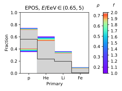
In Fig. 3 we show the composition obtained using a mixture model of 4 primaries, (p, He, N, Fe), using the EPOS hadronic model. The black line indicates the best fit, while the bars represent the allowed fractions at 95% CL. Different colors show the effect of including inferred values of , for different values of : the grey band obtained for , that is by doubling the size of the GH dataset, down to the purple one, where .
Similarly, in Fig. 4 we show the result for the full cumulative composition, that is for each primary we show the allowed fraction of heavier primaries, . We observe again an improvement of the grey region with respect to the purple.
We provide the same results for the hadronic models Sibyll, QGSJet01 and QGSJetII-04 in the Appendix.
V Conclusions
In this Letter we presented a novel method to improve the statistical power of GH events by including values of UHECRs inferred from SD observables. The effective number of events obtained is quantified by the variance ratio , which strongly depends on the level of correlation between ground and fluorescent data. While simple linear or non-linear fits can achieve at most correlation levels, resulting in rather modest values of , more advanced approaches can reach above correlation PierreAuger:2021fkf, leading to .
We then project the CR composition inference with such enhanced datasets, as a function of the ratio . The resulting projected improvements in the composition CL for the Auger Open Data are shown in Figs 3 and 4 and in the Appendix. Although the latter results seems meager, this study shows that, as a proof-of-concept, these improvements are possible and can be exploited by the experimental collaboration on their full dataset. Furthermore, it underlines the potential of probing deeper the correlation of SD and FD data, where the advancement in artificial intelligence tools can lead to interesting and powerful results.
Finally, we point out that the procedure to enhance the dataset by SD observables is very general and based on statistics arguments only. That is, any analysis based on correlated observables can make use of this method to augment a dataset containing measurements of both observables with (preferably a much larger) dataset of measurements of only a single one.33 3 For Pierre Auger, this could be advantageous i.e. in the exploration of observables to discriminate between hadronic models, a direction we leave for future work.
Acknowledgments
We are grateful to Gregor Šega for helping in reviewing the method outlined in the Letter. The authors acknowledge the financial support from the Slovenian Research Agency (grant No. J1-3013 and research core funding No. P1-0035).
Appendix A UHECR COMPOSITION FROM NON-HYBRID EVENTS
Below we present the projections of compositions for all hadronic models considered: EPOS (as in the main text), Sybill, QGSJetII-04 and QGSJet01 in the energy bin . In case of 4 primaries projections are shown in Fig. 5, while for 26 primaries are given in Fig. 6.


References
- (1) Pierre Auger, A. Aab et al., Nucl. Instrum. Meth. A 798, 172 (2015), 1502.01323.
- (2) T. P. A. Collaboration, Pierre auger observatory 2021 open data, 2021.
- (3) Pierre Auger, A. Aab et al., Phys. Rev. D 96, 122003 (2017), 1710.07249.
- (4) Pierre Auger, A. Aab et al., JINST 16, P07019 (2021), 2101.02946.
- (5) EAS-MSU, IceCube, KASCADE Grande, NEVOD-DECOR, Pierre Auger, SUGAR, Telescope Array, Yakutsk EAS Array, L. Cazon, PoS ICRC2019, 214 (2020), 2001.07508.
- (6) B. Bortolato, J. F. Kamenik, and M. Tammaro, Phys. Rev. D 108, 022004 (2023), 2212.04760.
- (7) B. Efron and R. J. Tibshirani, An Introduction to the Bootstrap, Monographs on Statistics and Applied Probability No. 57 (Chapman & Hall/CRC, Boca Raton, Florida, USA, 1993).
- (8) F. N. David and N. L. Johnson, Biometrika 35, 182 (1948).