Electric conductivity in non-Hermitian holography
Zhuo-Yu Xian1,2, David Rodríguez Fernández3-5,*, Zhaohui Chen1,2, Yang Liu1, René Meyer1,2
1 Institute for Theoretical Physics and Astrophysics, Julius–Maximilians–Universität Würzburg, Am Hubland, 97074 Würzburg, Germany
2 Würzburg-Dresden Cluster of Excellence ct.qmat
3 Instituut-Lorentz for Theoretical Physics, Universiteit Leiden, P. O. Box 9506, 2300 RA Leiden, The Netherlands
4 Instituto de Física Teórica UAM/CSIC, Calle Nicolás Cabrera 13-15, 28049 Madrid, Spain
5 Departamento de Física Teórica, Universidad Autónoma de Madrid, Campus de Cantoblanco, 28049 Madrid, Spain
*Corresponding author: david.rodriguez01@uam.es
Abstract
We study the phase structure and charge transport at finite temperature and chemical potential in the non-Hermitian -symmetric holographic model of [1]. The non-Hermitian -symmetric deformation is realized by promoting the parameter of a global symmetry to a complex number. Depending on the strength of the deformation, we find three phases: stable -symmetric phase, unstable -symmetric phase, and an unstable -symmetry broken phase. In the three phases, the square of the condensate and also the spectral weight of the AC conductivity at zero frequency are, respectively, positive, negative, and complex. We check that the Ferrell-Glover-Tinkham sum rule for the AC conductivity holds in all the three phases. We also investigate a complexified rotor model with -symmetric deformation, derive its phase structure and condensation pattern, and find a zero frequency spectral weight analogous to the holographic model.
1 Introduction
Non-Hermitian Hamiltonian evolution has attracted increasing interest in various areas of physics, including condensed matter, quantum information, and AdS/CFT, for reviews c.f. e.g. [2, 3]. In condensed matter, it has been widely employed in describing open quantum systems [4], for example as effective models of the finite quasiparticle lifetime introduced by electron-electron or electron-phonon interactions [5]. Furthermore, non-Hermitian descriptions have been employed in Weyl semimetals [6, 7, 8], for delocalization transitions or vortex flux line depinning in type II superconductors [9], as well as in the context of the interplay between topology and dissipation [10, 11]. In quantum information, non-Hermiticity has been introduced to describe projective measurements on quantum circuits or many-body systems, which turns out to be an efficient way to prepare entangled states [12, 13, 14, 15] and conduct quantum teleportation [16]. In AdS/CFT, it is also a potential route to a better understanding of the holography of complex spacetime metrics and of quantum matter [17, 18, 19, 20, 21].
Non-Hermiticity does not necessarily lead to a complex energy spectrum and non-unitary Hamiltonian evolution [22, 23, 3]. If a non-Hermitian Hamiltonian satisfies -symmetry, namely the Hamiltonian is invariant under the combination of a generalized time-reversal and a generalized parity transformation, it is possible that the spectrum remains real and unitary evolution still holds in terms of a new inner product. -symmetric theories have been extensively explored in the context of quantum mechanics [22, 23], quantum field theory [24, 25, 3, 26], and even classical physics [27]. If an eigenstate of the Hamiltonian is also a simultaneous eigenstate of the operator , then its energy is real. If it is not a eigenstate but part of a doublet, it is in general mapped to another state by the action of , with complex conjugate energy. Most -symmetric Hamiltonians are found to be pseudo-Hermitian, with eigenenergies appearing in complex conjugate pairs [28, 29]. The spectrum of a -symmetric Hamiltonian can hence be real, partially complex, or completely complex. If at least some energies are complex, the symmetry is spontaneously broken. A -symmetric Hamiltonian with a real spectrum can always be related to a Hermitian Hamiltonian via a similarity transformation [30, 28, 31, 32], the so-called Dyson map [33]. Recently, it has been observed that symmetry also plays an increasingly important role in strongly interacting systems relevant to holography, such as the Sachdev-Ye-Kitaev model [34, 35, 36, 37] and holographic quantum matter [1, 38].
In this work, we will focus on the electric conductivity of the -symmetric non-Hermitian model of [1]. Unitarity constrains transport phenomena in electron systems as well as in holography, for example by constraining the shear and bulk viscosities and , as well as the dissipative part of the electric conductivity to be positive semidefinite [39],
| (1) |
In the free Dirac fermion system with complex spectrum studied in [40], , and the conductivity sum rule holds. In this paper, we are going to investigate transport in strongly interacting non-Hermitian systems at zero or finite chemical potential via the AdS/CFT correspondence, which will provide predictions for transport coefficients in strongly coupled and correlated -symmetric systems. Different from standard computational approaches to interacting fermionic systems, AdS/CFT does not rely on perturbation theory, and does not suffer from the fermion sign problem.
| Phase I | Phase II | Phase III | |||
|---|---|---|---|---|---|
| symmetry | preserved | preserved | broken | ||
| (free) energy | real | real | complex | ||
| scalar stability | stable | unstable | unstable | ||
| vector stability | stable | stable | stable | ||
|
positive | negative | complex | ||
| QC conductivity | suppressed | enhanced | complex | ||
| FGT sum rule | holds | holds | holds | ||
| NEC | holds | violated | ill-defined |
In the model of [1], the non-Hermitian deformation is implemented by complexifying the global symmetry that is spontaneously broken in the Einstein-Maxwell-scalar model of [41]. As reviewed in Sec. 2.1, this effectively decouples the source for the charged scalar operator from its complex conjugate. This implements the Dyson map which connects a -symmetric Hamiltonian with real spectrum with an ordinary Hermitian Hamiltonian.
In this work, we further investigate the phase structure in the presence of the non-Hermitian -symmetric deformation at finite temperature and both at zero and finite chemical potential. The phase diagram at zero chemical potential is shown in Fig. 1 and discussed in detail in Sec. 2.3.2. The parameter , defined in (13), determines the strength of the non-Hermitian deformation. At zero temperature and vanishing chemical potential, is the symmetric phase, the exceptional point, and the broken phase of [1], respectively. At zero chemical potential, there are three finite temperature phases in the model of [1]: We not only reproduce the real solution in phase I and the pair of purely imaginary solutions in phase II found in [1], but also numerically construct a pair of complex conjugate solutions in phase III. The two complex conjugate solutions admit complex temperatures, and we check that their zero temperature limit approaches the two zero temperature solutions already found in [1]. The transition between phases II and III is a consequence of the competition between the thermal effect and the -symmetric breaking. The phase diagram exhibits the typical characteristics of quantum criticality of the -symmetric exceptional point. The phase diagram at finite chemical potential, discussed in Sec. 2.3.2 and shown in Fig. 4, is similar to the zero chemical potential case. We will comment on the interplay of superconductivity and breaking in Sec. 5.
The main results of our work are the calculation of the AC electric conductivity from linear perturbation theory, and the verification of the Ferrell-Glover-Tinkham (FGT) sum rule in each phase. The AC conductivity itself shows an interesting structure in phases I, II and III: In phase I the expectation value of the operator induces a positive superfluid density that leads to a contribution to and an associated pole in . In phase II, the superfluid density turns negative, . In phase III, itself becomes complex, leading to a contribution and a pole in both and . In general, the AC conductivity in holographic systems consist of three different parts, describing the effects of quantum criticality (incoherent transport), superconductivity, and coherent transport. They all contribute additively to the low frequency conductivity [42, 43, 44, 45, 46, 47, 48, 49, 50],
| (2) |
The incoherent conductivity is defined as the part of the conductivity unrelated to either momentum transport or condensation. Its limit is usually called the quantum critical conductivity, . In the weakly coupled limit, (and actually ) originates from the momentum-conserving scattering between electrons and holes [51] and is thus incoherent with the momentum flow, hence the name. The superconducting contribution is induced by the condensation of normal state charge carriers [52, 53, 54, 55], where is the charge of Cooper pairs. The coherent conductivity originates from the charge flow that is coherent to the momentum flow. In the absence of momentum relaxation, it has a contribution analogous to , as well as an analytic part. As electric charge is conserved, the charge carriers could contribute to all three parts of the conductivity by spectral weight transfer. As evident from Figs. 6, 7 and 8, we find that is reduced in phase I as compared to the AdS-Schwarzschild value , enhanced in phase II, and becomes complex in phase III. In Sec. 4, we study a complexified rotor model with the same -symmetric deformation as in [1], which reproduces the phases of the holographic model, and whose zero frequency spectral weight coincides with our results for the holographic model of [1].
Finally, we checked the validity of the FGT sum rule in all three phases. In ( boundary dimensions), at high frequencies the AC electric conductivity calculated in an asymptotically AdS4 background tends to a constant (in units of ), due to the scale invariance of the ultraviolet (UV) fixed point. Following [56], we subtract this constant, after which the FGT sum rule reads
| (3) |
We take the integral in (3) over the whole real axis, as the symmetry of conductivity under the transformation may not hold in the presence of non-Hermiticity. The subtraction is necessary for the integral to converge. The sum rule is expected to hold under the assumptions of causality, unitarity, and charge conservation [56]. It has been verified in various holography models [56, 57, 58, 47, 59, 60] fulfilling these assumptions. Since -symmetric non-Hermitian systems can break some of these assumptions, in particular unitarity in the -broken phase, we check the validity of (3) in the holographic model of [1]. We find that the sum rule holds in all three phases, even in the -broken phase.
This paper is organized as follows. In Sec. 2, we introduce the Einstein-Maxwell-scalar theory with the non-Hermitian -symmetric source deformation of [1], and study its phase structure at finite temperature and chemical potential. In Sec. 3, we calculate and discuss the AC conductivity. In addition, we verify the sum rule in each phase. In Sec. 4, we study a complexified rotor model with a -symmetric deformation. We find that its phase structure and zero frequency spectral weight turn out analogous to our holographic model. In Sec. 5, we present our conclusions and outline further research directions.
2 Non-Hermitian Holography
In this section, we first introduce the -symmetric non-Hermitian model of [1], and review its symmetries and the associated Dyson map, in Sec. 2.1. In Sec. 2.2, we present the equations of motion and the ansatz for the bulk fields that we will solve numerically in the remainder of this section for both vanishing (Sec. 2.3) and finite (Sec. 2.4) chemical potential.
2.1 Action and symmetries
In the AdS/CFT correspondence, every continuous global symmetry of the dual field theory is represented by a gauge symmetry in the bulk. Thus, while constructing the bulk theory, we at least need a gauge symmetry whose gauge field encodes the conserved current on the boundary. In addition, in order to implement the deformation of [1], a charged bulk field is needed. We follow the previous works [1, 38] and consider the scalar field to be minimally coupled, with charge under the symmetry. The holographic action reads
| (4) |
with and . In this paper we consider . The action (4) is the Abelian-Higgs model [54, 53]. It admits a local symmetry
| (5) |
The bulk action (4) is dual to a conformal field theory on the boundary with Hamiltonian . The local symmetry of the bulk action corresponds to the global symmetry of the boundary Hamiltonian . We identify the global symmetry with charge conservation.
We consider the field dual to an operator , and dual to . We introduce sources and for these operators, which corresponds to a deformation of the original Hamiltonian ,
| (6) |
If both and are related by complex conjugation, we have , and the deformed Hamiltonian (6) is Hermitian. The Gubser-Klebanov-Polyakov-Witten (GKPW) prescription relates the partition functions of the bulk and boundary theory and in the large and strong coupling limit, it reduces to a saddle point approximation,
| (7) |
Here we adopt standard quantization in which is the scaling dimension of given by one of the solutions of , is the radial coordinate, and is the conformal boundary. A nonzero source, either or , breaks the symmetry (5) and thus, charge conservation is violated on the boundary theory.
To explore non-Hermitian holography, we assume that the GKPW relation (7) still holds even for , and hence , while the holographic dictionary is preserved. Since , there are different ways to define the time evolution. We start with the Euclidean GKPW relation (7), in which the partition function is evaluated by the on-shell action on an Euclidean spacetime. In holography, the time evolution is usually chosen as follows:
| (8) |
In order to move to Lorentzian signature, one can perform a Wick rotation on the Euclidean spacetime. The observable measured on the asymptotic boundary of the Lorentzian spacetime at time , has therefore the the expectation value
| (9) |
Hence, the ordinary time evolution considered in holography is the analytical continuation of the Euclidean time path integral in the GKPW relation, which is different from other frameworks of non-unitary evolution in non-Hermitian systems [61, 62]. In Sec. 5, we will comment on the realization of these evolution schemes in holography. Nevertheless, if the theory has time translational symmetry, the one-point functions in (8) and (9) will be time independent, which is consistent with the construction of time-translational solutions in the bulk in this as well as previous works [1, 38].
On the other hand, the conjugation relation between the expectation values and does not necessarily hold for , since
| (10) |
The generalization to can be implemented by the global complexified transformations
| (11) | ||||
| (12) |
with . Both the bulk action (4) and also the boundary condition in (7) are invariant under (11) and (12). From the GKPW relation, the partition function is invariant under the transformation (11) and hence, is only a function of the invariant of (11), namely
| (13) |
This means that each value of the invariant labels a class of theories related by the complexified transformation (12). Denoting the generator of the global transformation as , the transformation (11) can be achieved via the similarity transformation
| (14) |
where the sources transform in the same way as in (12). So we call it the Dyson map as well. will in general be non-Hermitian even though is Hermitian. Then, the evolution operator could be non-unitary even though the evolution operator is unitary. Still, the two evolution operators are similar via the Dyson map (14). The similarity transformation preserves the trace and the eigenvalues, so it leaves the partition function (13) invariant. Thus, all the theories with have entirely real eigenvalues, since they are similar to a theory with , whose Hamiltonian is Hermitian.
However, there are more general choices of with a real invariant , which can be either or . Since is invariant under the Dyson map (14), the case can not be mapped to a Hermitian Hamiltonian by the Dyson map (14), which would require . Thus, is the exceptional point. We now show that in all these cases, the holographic theory is -symmetric with a proper parity . See App. A for a fermion model example with symmetry.
Firstly, given a theory with , it is -symmetric with the following transformation rules of and [1, 38]
|
|
without exchanging the sources . In other words, after the action of , is sourced by and is sourced by ; after , is sourced by and is sourced by . If , then both the bulk action and the boundary condition are invariant under this transformation. A theory with defines a ‘standard’ frame with respect to the complexified transformation, as it entails a ‘standard’ definition of the transformation, defined in (2.1).
Secondly, given a theory with , but , we can parameterize the sources as and with . Then, this theory is exactly the image of the theory with under the complexified transformation (12) with angle . The former Hamiltonian is similar to the latter Hamiltonian via . Since and [3], is invariant under a new transformation with . Starting from the ‘standard frame’ with , in any other complexified frame, there will be a correspondingly transformed definition of under which the theory is invariant in this frame.
We conclude that each value of the invariant labels a class of -symmetric theories related by the complexified transformation. Without loss of generality, we can pick a representative in each class with a gauge 11 1 In Ref. [1], the authors parameterized the complexified transformation (12) as and the invariant as , where and are real numbers. Thus, changing with fixed in their paper is simply changing along the real axis in our paper. Especially, their regions , , and correspond to our regions , , and , respectively.
| (19) |
In this gauge, we will show that holds for the solutions in all three phases.
Now we discuss the symmetry of the solution. Similarly, to labelling a class of Hamiltonians, each profile of labels a class of solutions related by complexified transformation (11) in the bulk. The transformation (2.1) maps . Thus, given a solution with , the symmetry is preserved by the solution; given a solution with , the symmetry is spontaneously broken by the solution.
2.2 Equations and ansatz
We now discuss in detail the equations of motion and the ansatz for the background solution. In our numerical calculation, we set the mass of scalar field to be and to ensure an analytic FG expansion near the conformal boundary. In addition, we choose the coupling coefficient . The equations of motion read as follows,
| (20) | ||||
| (21) | ||||
| (22) | ||||
| (23) |
where we have made use of the on-shell trace of the Einstein equations.
In this paper, we investigate static and translationally invariant solutions for the background, and hence the following metric and gauge field ansatz [1]
| (24) |
Since we choose , the scaling dimension of the dual scalar operator can have two cases or , which depends on the choice of quantization. Here we work in standard quantization, and thus identify . In this setup, the source is identified as the leading coefficient in the asymptotic expansion form of the scalar field
| (25) |
If working in alternate quantization with , one should do the exchange . Since neither nor exchanges the sources , the expansion after the transformation is
| (26) |
and after the transformation is
| (27) |
Clearly, a nonzero source or explicitly breaks the symmetry (5). For a static solution, we note that the component of the Maxwell equation (21) requires
| (28) |
Thus, the Ward identity
| (29) |
vanishes. is the charge current and is the coordinate index on the boundary. The Ward identity (29) can also be obtained by taking the derivative of (13) w.r.t. . The vanishing of (29) in spite of the explicit symmetry breaking is due to the fact that the divergence of the current is evaluated on a static solution.
Notice that the complexified invariant combination is . As explained in detail in Sec. 2.1, in order to label the equivalence class of partition function , we define with the condition . Without loss of generality, we can still rotate the sources to be utilizing the complexified transformation. By this rotation, both the equations of motion and boundary condition are invariant under the exchange of . With (28), we can further consider the following ansatz for the scalar fields
| (30) |
where is invariant under the complexified transformation. The ansatz (24)(30) is invariant under the rescaling
| (31) |
Substituting the above ansatz into the equations of motion, we obtain four independent equations
| (32a) | ||||
| (32b) | ||||
| (32c) | ||||
| (32d) | ||||
and one constraint [52]
| (33) |
whose value on the horizon will give the Hawking temperature . The null energy condition (NEC) is given by
| (34) |
which could be violated once becomes negative.
We consider the asymptotic boundary conditions
| (35) | ||||
with the chemical potential, the charge density, and is related to the energy density, and we have normalized the expectation value according to the convention in [53]. So is invariant under the complexified transformation. At finite temperature, we denote the horizon as and impose regularity there, namely,
| (36) |
The Hawking temperature is defined by
| (37) |
where refers to . The entropy density is . From the holographic renormalization given in App. F, which follows from [63, 64, 65, 66], the grand canonical potential density , free energy density , and energy density can be formulated as
| (38) |
which we find more convenient for numeric calculation. Following the rescaling transformation (31), both the sources and observables change as
| (39) |
Hence, it is convenient to rescale to be unit and parameterize the solutions with dimensionless ratios . We present both the neutral case with and the charged case with in the following two subsections.
2.3 Neutral background
In this subsection, we construct and characterize the three different phases of the holographic model (4) for vanishing chemical potential , and finite deformation sourced by . We find three different phases, labelled by I, II and III. While the phases I and II have been found already in [1], the finding of phase III is novel.
2.3.1 Fixed points and zero temperature solutions
Prior to our analysis at finite temperature, we examine the fixed point and RG structure at zero temperature. In the neutral case with , the Maxwell equations (32c) with the boundary conditions are solved by globally.
We first analyze the fixed points structure and find the zero temperature solution. According to [67, 52], the model (4) at zero chemical potential has three AdS4 fixed points,
| (40) | ||||
| (41) |
The UV fixed point is dual to an AdS4 space. Since , the deformation in (6) is relevant. The IR fixed points are dual to two AdS4 spaces with constant scalar field. The IR± are related by the complexified transformation (11), which could be reached by the RG flow triggered by a nonzero source .
The interpolation between these fixed points is given by the solutions at zero temperature. We can numerically solve the equations of motion (32) in the limit or directly work in the domain-wall coordinate [67, 52, 68]. In Fig. 2, the solutions for the scalar field are plotted in the complex plane, i.e. in an invariant way under the complexified transformation (11). We find one real solution for and two complex conjugate solutions for , reproducing the result of [1]. Our numeric calculation yields the free energy density, which coincides with the energy density at zero temperature, and in the two branches respectively. The free energy is real when and imaginary when . The real solution preserves the symmetry and the complex solutions break the symmetry. We will see that they are, respectively, the zero temperature limits of phase I and phase III defined in the next section. The real solution, illustrated by the blue RG flow in Fig. 2, preserves NEC (34), and the RG flow accordingly satisfies the holographic c-theorem [69, 70]. On the other hand, the complex solutions, illustrated by the green RG flow in Fig. 2, make the left-hand side of the NEC (34) complex. So there is no meaning to the c-function derived from the scale factor in the holographic c-theorem. But the resulting background geometry becomes real AdS4 both in the UV and IR limit, in which the inequality for the central charges as read from the scale factor is still fulfilled. At the exceptional point, the scalar decouples and the background geometry is an AdS4 fixed point.
Besides these three solutions, there are families of solutions in the complex plane that can interpolate the fixed points but do not satisfy the boundary condition . These are related, via the complexified transformation (12), to the case.
2.3.2 Phase diagram at finite temperature
We also numerically solve the equations of motion (32) at finite temperature. In virtue of the rescaling symmetry (31), we can fix the horizon radius to . This allows to determine the solutions as functions of only the radial coordinate and the dimensionless ratio . We perform the numerical integration of the equations (32) with the boundary conditions (35) and (36) at a specific value of . The temperature is determined from (37). We investigate the phase structure by varying the values of , and plot the expectation value for the scalar operator , free energy density , and energy density in Fig. 3. We find the following phase structure:
- Phase I
-
In the region , we find one branch of real solutions, which manifestly preserves the symmetry. The expectation value is real and negative. The solution in the limit coincides with the analytical approximation given in Sec. 2.3.3. The solution in the limit asymptotes to the real solution at zero temperature given in Sec. 2.3.1. In addition, NEC is also preserved for all values of . The observed increase in the energy density and the free energy density with increasing is expected, since we introduce a source in the boundary field theory.
- Phase II
-
In the region , there exist two branches of solutions with real metric and imaginary scalar field values [1]. The expectation value is purely imaginary. Even though is negative, these solutions still preserve symmetry. For , we numerically find a critical ratio . As in [1], these two branches are both unstable in the sector of scalar perturbations. In addition, NEC is violated in this case. Interestingly, the branch connected to phase I has a higher free energy density, but a smaller energy density in comparison to the other branch.
- Phase III
-
In the region of , we do not find any solution with real and real metric. However, if we allow the fields to take complex values, we do find a pair of complex conjugate solutions with complex and complex metric, for which symmetry is spontaneously broken. We extract two complex conjugate temperatures from imposing regularity on the horizon. The solutions in the limit asymptote to the two complex solutions at zero temperature discussed in Sec. 2.3.1. The expectation value , free energy , and energy density are complex. Also, the left-hand side of NEC (34) becomes complex. From the quasi-normal mode (QNM) analysis presented in App. (B), the two complex conjugate branches are also unstable.
We now discuss the complex metrics and complex temperatures in phase III in detail. For both solutions in phase III, the metric we calculate numerically has the following asymptotic behavior
| (42) |
Here , , and we omit the spatial coordinates. From imposing regularity at the horizon, the coordinate time acquires a complex period, with . If we define a new Euclidean time direction such that it has periodicity , the metric becomes
| (43) |
We see that the line element on a boundary cut-off slice is now complex,
| (44) |
where is the boundary time and is the UV cutoff. Eq. (44) implies a complex inverse temperature in the partition function
| (45) |
Complex metrics and complex time periods are not exotic in holography. In App. D, we review the “double cone” geometry contributing to the spectral form factor, which also admits complex line element on the boundary, and an interpretation involving a complex temperature.
The two complex conjugate solutions in phase III correspond to partition functions with two complex conjugate inverse temperatures,
| (46) |
Their related complex free energies and complex internal energies are shown in Figs. (3(b)) and (3(c)). We further checked explicitly that the limit of the two finite temperature solutions in phase III approach the two zero temperature solutions of [1] discussed in Sec. 2.3.1. Note that the zero temperature limit generally has to be taken along either of the two complex trajectories shown in Fig. 3(d) corresponding to the two solution branches.
Our holographic interpretation involving complex temperatures in phase III also resolves the following puzzle: The solutions in phase III have complex energies. However, since the -symmetric Hamiltonian (6) in holography is pseudo-Hermitian, even in the -broken phase, both the partition function , as well as the thermodynamic average of the energy , should be real for real . This apparent contradiction is resolved by concluding that the correct definition of the temperature must be complex in order to avoid a conical singularity at the horizon, and hence both partition functions in (46) are complex conjugate to each other.
The emergence of complex temperatures in the -broken phase is also expected in -symmetric non-Hermitian systems. This can be seen even in the two-level system analyzed in detail in App. E, where we show that the free energy encounters a branch cut when the temperature is lowered. When the branch cut appears, one should select one branch of the two complex conjugate temperatures, as the -broken phase is entered. The zero temperature limit is taken by fixing a nonzero argument of and sending , which reduces both the free energy and the average energy to one of the eigenenergies.
2.3.3 The probe limit
We can solve the scalar equation (32d) analytically when the source of the scalar field in is small compared to the temperature . In this situation, the bulk geometry can be approximated as an AdS4-Schwarzschild black hole with a scalar field in the probe limit, i.e. the propagation of this field does not alter the bulk geometry to leading order in . The AdS4–Schwarzschild solution is given by
| (47) |
The equation (32d) reduces to
| (48) |
This equation admits a solution regular at the horizon,
| (49) |
with the asymptotic behavior
| (50) |
From the near boundary expansion, we find
| (51) |
which matches the numerical result given in Fig. 3(a) in the limit .
2.4 Charged backgrounds

In this subsection, we discuss the case of finite chemical potential and derive the charged background solutions numerically. Due to the relation (30) derived from the Maxwell equation, for a given solution at finite , the counterpart with can be obtained just by changing the sign of , while keeping other fields fixed. So, and without loss of generality, we restrict to the case.
From the background solutions, we study the phase structure in the (, ) plane numerically. This is shown in Fig. 4. In particular, we find that the global phase structure above is similar to the neutral case in Fig. (1).
Below , the system has the superconducting instability of the scalar field of [53, 54]. When , this is a second-order phase transition, while for , the transition becomes a cross-over, namely, the VEV grows smoothly from a non-zero value below the critical temperature. For the holographic superconductor, this crossover was studied in [71]. Since the transition temperature is very small, we do not display it in Fig. 4.
3 Conductivity and the sum rule
In this section, we study the linear response of the model (4), and derive the AC conductivity. We consider the Kubo formula of conductivity
| (52) | ||||
| (53) |
where is the retarded Green’s function, is a positive infinitesimal number, and the time evolution is defined in (9). We will compute the longitudinal conductivity with and check the validity of the sum rule numerically.
The complexified transformation (11) does not change the Maxwell field . Thus, the charge current operator , and also its correlation function, are both invariant under the Dyson map
| (54) |
This invariance also holds for the fermion model presented in App. A. In order to calculate the conductivity from holography, we work in the gauge (19). In addition, notice that the perturbation equation (62) relevant for the conductivity depends on the scalar fields via the complexified invariant profile only. Therefore, in phase I, we expect the derivation of the AC conducitivity to be equivalent to the Hermitian case. The invariance of Dyson map in holography also supports our definition of evolution and Green function (53).
However, since the theory with is not similar to a Hermitian theory via Dyson map (14), the conductivity relation
| (55) |
may not necessarily hold in the region. Remarkably, we will show that (55) is a necessary condition in order for the sum rule to hold.
We firstly check the sum rule (3) by analyzing the properties of the retarded Green’s function of the charged current following [56]. As required by causality and the asymptotic behavior of the retarded Green’s function for the sum rule to hold, the following two conditions must be met:
- 1.
is analytical on the upper half plane and on the real axis;
- 2.
.
The first condition can be checked from the QNM spectrum in the holographic model, which will be done at the end of this section. The second condition is related to the asymptotic behavior of in the high frequency limit, which for this model becomes the current Green’s function of the AdS-Schwarzschild black hole without any scalar fields. By applying Cauchy’s theorem, we have
| (56) |
Adding up the first integral and the complex conjugate of the second integral leads to the spectral representation
| (57) |
Setting and using the Cauchy principal value integral, we obtain the sum rule (3).
In order to check the sum rule numerically, we also need to introduce the integrated spectral weight ,
| (58) |
In particular, notice that is exactly the sum rule (3). In the pure AdS-Schwarzschild case, it vanishes exactly regardless of . A non-zero value of (3) would signal a severe breakdown of either causality, unitarity, or charge conservation, due to the - and -invariance violation in the model (4).
3.1 AC conductivity
As the time evolution (9)(52) realized in AdS/CFT is of the same form as in the Hermitian case, we follow the standard procedure to derive the conductivity within the AdS/CFT correspondence [72] from linear gauge field perturbations. We consider the fluctuations of the gauge field and metric component
| (59) |
in the equations (20)-(23). The only non-trivial equations come from the component of the Einstein equations and the component of the Maxwell equations, which read
| (60) | ||||
| (61) |
The mix between and indicates a coupling of charge current and momentum. Solving (60) for and substituting it in (61), we get a single equation for
| (62) |
Imposing the ingoing boundary condition at the horizon
| (63) |
and requiring the regularity of near , we get the retarded Green’s function . From the Kubo formula (52), we get
| (64) |
The infinitesimal shift accounts for the delta peak at in the real part of the conductivity, which is essential for examining the validity of the sum rule (3). In the high frequency limit, namely , the conductivity approaches , as expected for the AdS-Schwarzschild geometry that governs the UV, while the low frequency behavior depends on the IR geometry. The low-frequency behavior is governed by the Kramers-Kronig (KK) relation, with two contributions denoted by and in such a way that
| (65) |
where is the superfluid density and is the normal charge density. Next, we present the numerical results of the AC conductivity on both the neutral and charged backgrounds and further analyze the asymptotic behaviors at high and low frequencies.
3.2 Numerical results

We first calculate the conductivity on the neutral background, i.e. . The conductivity shown in the left panels of Figs. 6, 7 and 8 correspond to phase I, II and III respectively. The right panels of these figures show the convergence of the integral (58), which is used to check the validity of the sum rule.
In the high frequency limit, there exists a common asymptotic behavior for all phases, , or for . This is exactly the conductivity for the asymptotic AdS-Schwarzschild background in the UV regime. In the right panels of Figs. 6, 7 and 8, we also observe that the integral in (58) always exhibits a power-law decay at , which confirms that the sum rule always holds. As an independent check, we also show that the sum rule holds from the quasi-normal modes spectrum at the end of this section.
In the low frequency limit, the conductivity agrees with our expectation (65) with due to the neutrality of the background. We extract from fitting the numerical conductivity and show it as a function of the square of the condensate in Fig. 5. In particular, we find for small . Therefore, the low frequency behavior of conductivity varies with the particular phase considered, with the following properties:
- Phase I
-
In this phase, we find that can be approximated as with at low frequencies. Due to the form (65), the conductivity satisfies the relation (55), as required by Hermiticity. In addition, the regular part of fulfills . This is required by the existence of a positive weight of the function due to the sum rule.
- Phase II
-
In this phase, can still be approximated as at small , except that now . Since , the conductivity still satisfies the relation (55). Furthermore, we observe that the analytical part of fulfills , which is also required by the existence of a negative weight of the function in the sum rule.
- Phase III
-
In this phase, we find that at small but nonzero with . Our numerical analysis finds that , and hence both and have behavior. Consequently, the conductivity does not satisfy the relation (55). Instead, the conductivity on the one branch of the background is mapped to the one on its conjugated branch under the change by (55). This requires to include in both the real and imaginary parts as well.
The symmetry is preserved in phases I and II, but broken in phase III. This breaking leads to the emergence of the complex weight and thus, to the breaking of the symmetry (55) of the conductivity under the reflection . Still, the sum rule always holds. The analytical study of conductivity in the probe limit in App. C also confirms the sum rule and shows that the superfluity density is proportional to the scalar field source, .
We also investigated the conductivity for finite chemical potential . By inspecting Fig. 9, we can observe, as we dial , a competition between the superfluid density and normal charge density in the low frequency limit (65) in phase II. The weight can be either negative or positive. Nevertheless, the sum rule always holds, as illustrated in the right plot of Fig. 9. The combination of also appears in phases I and III numerically.
3.3 Sum rule from quasi normal mode
We already observe the power law decay of the integral numerically in last subsection. In this subsection, we doubly check the first condition for the sum rule, stability, namely being analytic both on the upper half plane and the real axis. The poles of are given by the QNMs of the components [57]. For our numerical analysis, we arrange the differential equation (62), the boundary conditions (63) and together as a linear differential operator of the form
| (66) |
If the determinant of (66) vanishes for a set of frequencies, we found a QNM. One can write the operator as a matrix and calculate the . In Fig. 10, we plot this quantity as a function of the complex frequency, and infer that there is no pole on the upper half plane and the real axis. This shows that the retarded Green’s function is analytic both on the upper half plane and the real axis. Therefore, the first condition for the sum rule mentioned in Sec. 3 is satisfied. By combining it with the asymptotic condition for due to the UV fixed point, we independently confirm that the sum rule holds in all the phases.


4 Field theory: rotor model
To better understand phase III, in which the complex superfluity density emerges in the -symmetric holographic model, in this section, we construct an effective model in field theory which reproduces the phase transitions and the zero frequency spectral weight of conductivity found in the holographic model. We start from a rotor model with a charged scalar coupled to a gauge field . Then, we allow the scalar field to be independent from its complex conjugate , such that the original symmetry is complexified. We refer to this model as the complexified rotor model. After this, we break the complexified symmetry and also Hermiticity by introducing the -symmetric deformations. Its action in Minkowskian signature takes the form
| (67) |
where , and are two independent fields, is the mass square, is coupling constant, and are two independent sources, respectively. So this model is an analogue of the holographic model (4). Following (2.1), the application of transforms , and the application of transforms . Letting and considering a static and translational invariant solution to the scalar fields, the saddle point of the potential satisfies the following equations
| (68) |
where stands for the effective mass square. Similar to the holographic model, we can consider the complexified transformation,
| (69) |
Then, the saddle point solution follows the transformation rules
| (70) |
such that the on-shell action is invariant. This transformation preserves and , which enables us to choose without loss of generality. Once , the equations give . Finally, the on-shell action can be related to a -symmetric action via the complexified transformation if .
We restrict to the case, in order for the potential to be bounded from below for real ,. When , the action admits the global symmetry
| (71) |
If we set , the effective potential of looks like a Mexican hat with three extrema on the real axis. Then the symmetry will be broken spontaneously by the nonzero solution. However, in holographic approach (4), we consider an explicit breaking of the symmetry under the transformation (5). Thus, in order to establish an analogy to the holographic model, we consider . This entails that there is only one saddle point of the potential on the real axis. To break the symmetry explicitly and trigger nonzero solution, we turn on the source .
Around the resulting saddle point, we consider phase fluctuations and . The action in the small expansion is then given by
| (72) |
where plays the role of the superfluid density and the mass square of pseudo-Goldstone is
| (73) |
To study the dynamic stability around a saddle point , we consider a general fluctuation with and extract their effective mass square matrix . The linear perturbation equation in the frequency-momentum domain is
| (74) | ||||
| where |
are Pauli matrices and is the identity matrix. The zeros of the determinant of the coefficient matrix
| (75) |
determine the frequencies of zero modes. A stable saddle point requires real zeros, i.e. and vice versa. Thus, when , only those saddle points with are stable.
We always find three saddle points in the complex plane because of the quartic potential. Their movement depending on the value of is shown in Fig. 11. One of the saddle points remains a spectator, which does not merge with the others throughout the domain of parameters we study. We find three different phases as follows:
- Phase I
-
When , there is one real solution with , and two complex conjugate values of with . Only the real solution is stable.
- Phase II
-
When , there are three imaginary values of with . Only the solution connected to the real solution in phase I is stable.
- Phase III
-
When , there is one imaginary with and two complex conjugate values of with . All solutions are unstable.
The transition between phase II and phase III is due to the collision of two imaginary saddle points, which is analogous to the case in the holographic model. Going along those unstable directions, and will travel to another saddle point, move circularly or even flow to infinity.
In all phases, the current is
| (76) |
The Kubo formula in frequency-momentum space is
| (77) |
The superfluid conductivity along the direction is
| (78) |
The integral of the spectral weight is
| (79) |
which depends on the sources and via only. Notice that from (79), no actual violation of the sum rule can be deduced, as we are considering the phase fluctuation at quadratic order in (72) and ignoring the existence of loop corrections coming from both phase and absolute value (Higgs mode) fluctuations, which is the reason for the absence of the normal (not superconducting) contribution to the conductivity. In summary, the rotor model (67) reproduces the behavior of the condensate in all three phases found in the holographic model (4).
5 Conclusions
In this work, we studied the solution structure and AC conductivity for the non-Hermitian holographic model of [1], both at zero and at finite density. The solution space we examined consisted of the two sources of the complex scalar operator and , the temperature , and chemical potential . The -symmetric non-Hermitian deformation consists of effectively decoupling and , where in the usual Hermitian setup, is the complex conjugate of . The deformation switches on sources for the scalar operators and , which in the Hermitian case also are complex conjugate to each other. Both operators receive expectation values, i.e. condensates and . Note that the sources and break the symmetry explicitly, and not spontaneously as in the holographic superconductor of [41].
Within the explored solution space, there are two -symmetric phases at finite temperature with real (phase I) and imaginary (phase II) condensates, respectively, which have already been constructed in [1]. The finite temperature solutions in phase II approach the exceptional point in a zero temperature limit in which the ratio is held fixed. We furthermore calculated the free energy in phase II (c.f. Fig. 3(b)), and in this way identified the thermodynamically dominant solution branch. Since the exceptional point in the holographic model [1] is exactly AdS4, the phase diagram Fig. 1 suggests that phase II is actually part of a quantum critical region at finite temperature, which emanates from the quantum critical exceptional point at zero temperature.
We also presented and discussed in detail the emergence of a -broken finite temperature phase with complex condensates (phase III). We checked that our finite temperature solutions approach, in the zero temperature limit, the complex conjugate pair of extremal solutions constructed in [1]. A peculiar feature of our finite temperature solutions in phase III is that the metric sourced by the scalar field also becomes complex, while it remained real in phases I and II. Requiring the absence of a conical singularity at the horizon implies that the temperature acquires an imaginary part in phase III. While a complex temperature seems puzzling at first, as discussed in App. D, a similar phenomenon appears in the double cone geometry of JT gravity. In addition, we quantified the transition point from phase II to phase III, which occurs at a critical value of . We note that in general, this value is a function of the conformal dimension , the charge of the scalar field , and the coefficient of the quartic term in the action . For future work, it will be interesting to explore the parameter space thoroughly in order to further analyze the phase structure of deformed holographic Einstein-Maxwell-scalar theory [52, 73]. In addition, following [74] and analysing quantum critical points from the top-down perspective should be insightful as well.
Although the phase diagram in Fig. 1 is calculated in a holographic model, the overall phase structure with phase I, II, III is reminiscent of a quantum phase transition of a pseudo Hermitian system, where the symmetry is spontaneously broken due to collision between the two lowest energy eigenstates prior to any other states. Consider the energy eigenvalues as functions of the strength of the -symmetric deformation . For case, and satisfies , while for case, in which . The partition function is
For small , we have for any and then . Furthermore, for sufficiently low temperature , . Thus there are supposed to exist lines in the v.s. plane satisfying . The line with highest temperature will be the boundary between phase II and III, above which the system is in phase II with and , and below which it is in phase III with and , depending on the branches of . As an example, the same phase structure was also observed for the simple two-level system in App. E.
Furthermore, we calculated the AC conductivity for each of the three phases and observed a shift of spectral weight to a delta function at zero frequency as a function of the breaking parameter . Zero frequency spectral weight can be induced by the condensation of charged operators as well as by normal charge densities, with the latter being absent at zero chemical potential. We found that the zero frequency spectral weight induced by the condensate is positive in phase I, negative in phase II, and complex in phase III, leading to a delta function and a pole in both and . Still, in all three cases, a mode analysis in the channel related to the longitudinal charge transport shows that the Kramers-Kronig relations hold, as all quasinormal modes are in the lower half frequency plane. Moreover, the quantum critical conductivity, which is the DC limit of the real analytic part of the AC conductivity, is suppressed in phase I and enhanced in phase II, as compared to the value (in units of ) for the AdS-Schwarzschild solution [75]. We also extracted the quantum critical conductivity in phase III, finding a complex value for due to the breakdown of the relation (55) In contrast, if (55) holds, the imaginary part of always vanishes. We also observe that the FGT sum rule always holds from two perspectives: 1) as a direct integral of the real part of the AC conductivity, and 2) from the analysis of the quasi-normal mode spectrum. The sum rule holds both in the -symmetric and broken phases, and also at finite chemical potential, and is in essence responsible for the suppression or enhancement of the quantum critical conductivity due to the spectral weight in the pole. We would like to stress again that the sum rule holds in [40] due to a quite different reason: the symmetry remains unbroken and the charge conservation holds dynamically. Also the AC conductivity in [40] exhibits a hard gap at zero temperature, in contrast to the holographic superconductor [73].
We also constructed and analyzed a complexified rotor model with an analogous -symmetric deformation from effective field theory principles. By tuning the sources of the scalar operators, we find real, imaginary and even complex solutions. The nonzero sources break the symmetry explicitly, and pseudo-Goldstone bosons with a finite mass appear. We studied the AC conductivity in all phases of the rotor model. We found an analogous shift of spectral weight to the delta functions at zero frequency as in the holographic model. The spectral weight is given by the condensates. The rotor model also admits some differences to the holographic model: First, from (79), we find that the apparent violation of sum rule in all phases, as we only consider the phase fluctuation around the saddle point in the rotor model, instead of solving the whole model, including the absolute value of the scalar field. Second, as evident from the left panel of Fig. 11, in all three phases, the rotor model has one or more additional complex solution compared to the holographic model Fig. 3. However, this does not necessarily mean that the holographic model has another solution that we possibly missed in our numerical analysis. As all the properties of the solutions of the holographic model are reproduced by at most two solutions of the rotor model, it looks as if the additional solution in the rotor model is just a spectator which does not play any role in the universality argument.
For future work, it will be interesting to investigate -symmetric non-Hermitian versions of superconductivity in holography [76], and compare to recent field theory studies [77, 78, 79, 80, 81, 82, 83], as well as to holographic hydrodynamics [71]. Another interesting route is to further investigate -symmetric deformations of SYK-type models, following [84, 85, 86, 87, 88, 89]. We also studied the shear viscosity on the holographic background, and found that the KSS bound [90] is still saturated, as expected for an asymptotically AdS background. However, could behave non-trivially if we combine higher derivative corrections with PT symmetric non-Hermicity [91, 92]. Finally, it will be interesting to calculate the quantum critical conductivity from kinetic theory in a -symmetric Dirac metal along the lines of [93], in order to understand how sensitive is the suppression/enhancement feature we found in the holographic model to the coupling strength.
Moreover, it is interesting to study the entropy of the non-Hermitian model in holography. The pseudo entropies for non-Hermitian transition matrices of were studied [94, 95, 96, 97]. In non-Hermitian systems, the transition matrices were considered as instead of or as its convenience in path integral [98, 99], where and are the right and left eigenvectors with lowest real part of energy, respectively. Based on our analysis, when the ground state energies become a complex pair in the PT-broken phase, we could obtain the transition matrix by taking in the limit with a fixed imaginary angle of , which is exactly the zero temperature limit considered in this paper. Remarkably, we indeed found a solution with complex metric in phase III including the zero temperature limit in Sec. 4. So we could obtain an extremal area taking complex values according to the RT formula, which agrees with the pseudo entropy could take complex values [96].
Finally, in this paper, we use the standard GKPW relation (7) in Euclidean time and analytically continue it to Lorentzian time (9). This defines a particular holographic time evolution in the presence of the deformation. Alternatively, some studies [100, 61, 62] consider a Hermitian density matrix such as the Gibbs state , and define real time evolution as with the non-Hermitian Hamiltonian . Correspondingly, the Heisenberg picture of an operator becomes , and the expectation value will in general be time-dependent,
| (80) |
Obviously, this is different from the holographic construction considered here and in [1], where the background solutions are all static, i.e. time-independent. Also, the evolution in (80) will not be invariant under the complexified transformation, as for a general . To compute the expectation value (80) with and the non-Hermitian Hamiltonian in (6) in holography, we could first prepare an Euclidean black hole at temperature without sources, next apply a quench on one side with for time and a quench on the conjugate side with for time , then measure the observable , and finally glue the two sides together following [101, 102]. We leave it for future work [103].
6 Acknowledgements
We thank Daniel Areán, Matteo Baggioli, Sebastian Grieninger, Ren Jie, Viktoriia Kornich, Karl Landsteiner, Ronny Thomale and Björn Trauzettel for useful discussions. The work of Z. Y. X., D. R. F., Z. C. and R. M. was funded by the Deutsche Forschungsgemeinschaft (DFG, German Research Foundation) through Project-ID 258499086—SFB 1170 “ToCoTronics” and through the Würzburg-Dresden Cluster of Excellence on Complexity and Topology in Quantum Matter – ct.qmat Project-ID 390858490—EXC 2147. The work of Y. L. is funded through a PhD scholarship of the Studienstiftung des deutschen Volkes. D.R.F. is also supported by the Dutch Research Council (NWO) project 680-91-116 (Planckian Dissipation and Quantum Thermalisation: From Black Hole Answers to Strange Metal Questions), the FOM/NWO program 167 (Strange Metals) and through the grants SEV-2016-0597, PGC2018-095976-B-C21 and “María Zambrano para la atracción de talento” CA3/RSUE/2021-00898. Z. Y. X. also acknowledges support from the National Natural Science Foundation of China under Grants No. 11875053 and No. 12075298. Z. C. is also funded by China Scholarship Council.
Appendix A A fermion model with symmetry
In this appendix, we will give a simple model with symmetry, and to be specific, consider the dimensional Hamiltonian of fermion as in [104],
| (81) | |||
| (82) |
with and . In dimensional spacetime, the conventions are adopted as follows,
| (83) |
where are Pauli matrices. To relate it to the symmetry in the main text, one can consider a redefinition of operators as the last step of (81). The actions of and transformations on the fermion are
| (84) | |||
| (85) |
The transformations on the scalar and pseudo-scalar are the following,
| (86) | ||||
| (87) | ||||
| (88) | ||||
| (89) |
So obviously, the Hamiltonian is Hermitian and also satisfies and symmetries, respectively
| (90) |
Furthermore, we consider the the charge transformation and chiral transformation
| (91) |
respectively. The theory is invariant under the charge transformation for general and is invariant under the chiral transformation when . The charge current and axis current corresponding to these symmetries are respectively
| (92) |
both of which are Hermitian. Although the chiral symmetry is broken when , the Ward identity still vanishes, i.e.
| (93) |
where denotes . It shares the same feature as the holographic Ward identity (29).
To construct non-Hermitian -symmetric Hamiltonian, one can define the Dyson map as the chiral transformation with the generator being the (rescaled) axis charge
| (94) |
So the Dyson map transforms the scalars as the following forms [104]
| (95) |
with . Ultimately, the Dyson map transforms the Hamiltonian into a non-Hermitian one
| (96) |
where
| (97) |
Now we realize that the Dyson map corresponds to a complexified transformation, which is analogous to (12). Consequently, both and are invariant under the complexified transformation. The original theory has the non-negative invariant . However, we could generalize it to the whole real axis . The source terms in share the same form as the holographic model (4) and rotor model (67).
One can check that both of the currents in (92) commute with . Thus, their transports are invariant under the Dyson map.
The with is invariant under the combination of another and transformations. We define a new parity as
| (98) |
is non-Hermitian but is -symmetric, namely
| (99) |
where we have used [3].
Appendix B Instability analysis
We study the stability of the solution in holography by examining the QNM. Following [1], we only consider the perturbation on the matter fields, as this set will provide a consistent set of equations alone. The following ansatz of perturbations is introduced
| (100) |
so that the perturbation on energy-momentum tensor vanishes, that is . The perturbation equations are
| (101) | ||||
| (102) | ||||
| (103) |
From applying local gauge transformation, we find that
| (104) |
is always a solution. To calculate the QNM on the asymptotic boundary, we require zero sources up to the gauge transformation (104), namely
| (105) |
Near the horizon, we impose ingoing boundary conditions and find the following expansions
| (106) | ||||
| (107) | ||||
| (108) |
where the two coefficients and are determined by the asymptotic boundary conditions (105).
Given a background solution, frequency and momentum , we can transform the QNM of the perturbation equations (101) and the boundary conditions (105)(106) into the null vector of a matrix . By finding the poles of in the complex plane with a given , we can find the QNM. We show the most important pole in Fig. 12, where the frequency could cross the upper half plane at low momentum, which would signal the onset of the instability. However, we find that this mode triggers a shift on the chemical potential with .
Appendix C Analytic conductivity in the probe limit
We aim here to derive an approximate expression of the conductivity and study the sum rule on the neutral background with small source. For this, we disregard the normalizable mode in the near boundary for the scalar field in the equation (62), so that 22 2 We thank Jie Ren for helpful discussions and comments.. Adopting the notation and rescaling , we rewrite (62) as
| (109) |
where is positive (negative) in phase I (phase II). The solution of this differential equation is expressed in terms of the Heun function
| (110) |
where is an integration constant and . The retarded Green’s function and the conductivity are found to be
| (111) |
and
| (112) |
where the prime in the numerator denotes the -derivative. In the low frequency limit, the conductivity takes the form
| (113) |
This result is compatible with (65) at (notice that this implies ), and the leading term of takes .
The limit we take in this section is equivalent to , within this constraint we found out that the sum rule still holds. As can be seen from Fig. (13), in the high frequency regime, the integrated spectral weight (58) decreases in power law (left) and there is no pole in the upper-half plane and the real axis of the complex frequency (right). This justifies the two conditions from [56].

Appendix D Complex temperature of the double cone geometry
Complex metrics and complex time periods are not rare in holography. We take the double cone geometry in [17] as an example, where the bulk theory is JT gravity and the boundary theory is a Schwarzian action with a Hermitian Hamiltonian . The double cone geometry is dual to the ramp of the spectral form factor (SFF) of the boundary theory
| (114) |
which has complex inverse temperatures and . The ramp in the connected part of SFF is contributed by a semiclassical double cone geometry, with metric
| (115) |
where the periodicity defined in [17], is the auxiliary inverse temperature parameterizing the solutions that contribute to the ramp. For the right factor in (114), the induced metric on the right UV cutoff slice of the double cone geometry satisfies the boundary condition
| (116) |
Upon identification of , this agrees with a complex period in , where a possible real factor was absorbed into . In summary, both of the line elements in (44) and (116) are complex, and hence the coordinates in (44) and in (116) play the similar roles.
Appendix E A two-level system with symmetry
Here we review the non-Hermitian two-level model with symmetry and discuss the symmetry breaking at finite temperature. Consider a non-Hermitian Hamiltonian of two-level system
| (117) |
where and are Pauli matrices. It is -symmetric with being parity and being the complex conjugate. The eigenvalues are . They are real when and imaginary when . So the symmetry is spontaneously broken at zero temperature when .
Consider the canonical ensemble at finite temperature . The partition function, free energy, energy, and average entropy are respectively
| (118) | ||||
| (119) | ||||
| (120) | ||||
| (121) |
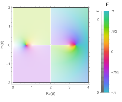
We plot on the - plane in Fig. 15. We call the region of phase I, in which the spectrum and the free energy are both real. The region of and is phase II, in which the spectrum is complex but the free energy remains real. The region of and is phase III, in which the spectrum is complex and the free energy encounters the first branch cut along the real axis of at , as shown in Fig. 15. must deviate from the real axis and continue to the upper or lower half plane such that takes complex conjugate values on the two half planes. The phase structure presented in Fig. 15 is analogous to that in the holographic model as shown in Fig. 1. The emergence of complex temperature on the phase boundary between phases II and III also evokes the complex solutions with complex temperatures, as we find in holography.
Furthermore, in order to get the eigenvalues from the canonical ensemble in the zero-temperature limit, we could introduce an imaginary angle to the inverse temperature with and send . Taking the branch from analytical continuation, we get the two eigenvalues from both free energy and average energy ,
| (122) |
Similar limit behavior appears in the holographic model where the limit of the solutions in phase III gives the zero temperature solutions.

Appendix F Holographic renormalization
By using the holographic renormalization in [105, 106], we can determine the thermodynamic quantities including the grand potential density , charge density , energy density , and pressure . We follow the same approach as in [92, 107]. Firstly, in order to derive the on-shell action , we need the extrinsic curvature and scalar , which are defined by
| (123) |
where is the induced metric on a constant slice, where stand for the indexes. Inserting the on-shell relation for the Ricci scalar,
| (124) |
into the action (4) and after some further manipulations, we arrive at33 3 In this section, as well as in the whole work, we employ units.
| (125) |
where the first term is split into two surface integrals on the boundary and horizon from Gauss theorem. The action (125) diverges when . This can be canceled by adding the following boundary counterterms (we set )
| (126) |
so that the renormalized action in (7) reads
| (127) |
Near the boundary (), the bulk fields read
| (128) | ||||
To express the horizon integral in (125) in terms of the boundary data, we evaluate the constraint equation (33) on the boundary and horizon, namely
| (129) |
where is the black hole temperature and is the entropy density. Finally, we express the renormalized action (127) in terms of the boundary data, obtaining
| (130) |
The remaining thermodynamic quantities can be determined by considering variations of the of the renormalized action with respect to the boundary sources
| (131) | ||||
| (132) | ||||
| (133) | ||||
| (134) |
where is the Brown-York tensor. Evaluating the expressions (131)-(134) at the boundary by means of the expansions (F) yields
| (135) | ||||
| (136) | ||||
| (137) | ||||
| (138) | ||||
| (139) |
From here, we notice that the pressure , as expected. In addition, the Ward identity for the trace of the stress tensor reads
| (140) |
which has the expected form. Furthermore, after combining (135) and (136), we find the Gibbs-Duhem relation
| (141) |
where we have made use of the constraint (129), as well as of (139).
References
- [1] D. Arean, K. Landsteiner and I. S. Landea, Non-hermitian holography, SciPost Physics 9(3) (2020).
- [2] E. J. Bergholtz, J. C. Budich and F. K. Kunst, Exceptional topology of non-hermitian systems, Reviews of Modern Physics 93(1) (2021).
- [3] C. M. Bender, Making sense of non-hermitian hamiltonians, Reports on Progress in Physics 70(6), 947 (2007).
- [4] Y. Michishita and R. Peters, Equivalence of effective non-hermitian hamiltonians in the context of open quantum systems and strongly correlated electron systems, Physical Review Letters 124(19) (2020).
- [5] T. Yoshida, R. Peters and N. Kawakami, Non-hermitian perspective of the band structure in heavy-fermion systems, Physical Review B 98(3) (2018).
- [6] Y. Xu, S.-T. Wang and L.-M. Duan, Weyl exceptional rings in a three-dimensional dissipative cold atomic gas, Phys. Rev. Lett. 118, 045701 (2017).
- [7] A. A. Zyuzin and A. Y. Zyuzin, Flat band in disorder-driven non-hermitian weyl semimetals, Phys. Rev. B 97, 041203 (2018).
- [8] A. Cerjan, M. Xiao, L. Yuan and S. Fan, Effects of non-hermitian perturbations on weyl hamiltonians with arbitrary topological charges, Phys. Rev. B 97, 075128 (2018).
- [9] N. Hatano and D. R. Nelson, Localization transitions in non-hermitian quantum mechanics, Phys. Rev. Lett. 77, 570 (1996).
- [10] M. S. Rudner and L. S. Levitov, Topological transition in a non-hermitian quantum walk, Phys. Rev. Lett. 102, 065703 (2009).
- [11] J. C. Budich and S. Diehl, Topology of density matrices, Phys. Rev. B 91, 165140 (2015).
- [12] M. Block, Y. Bao, S. Choi, E. Altman and N. Yao, Measurement-Induced Transition in Long-Range Interacting Quantum Circuits, Phys. Rev. Lett. 128(1), 010604 (2022), 2104.13372.
- [13] A. Zabalo, M. J. Gullans, J. H. Wilson, S. Gopalakrishnan, D. A. Huse and J. H. Pixley, Critical properties of the measurement-induced transition in random quantum circuits, Phys. Rev. B 101(6), 060301 (2020), 1911.00008.
- [14] S.-K. Jian, C. Liu, X. Chen, B. Swingle and P. Zhang, Measurement-Induced Phase Transition in the Monitored Sachdev-Ye-Kitaev Model, Phys. Rev. Lett. 127(14), 140601 (2021), 2104.08270.
- [15] R. Fan, S. Vijay, A. Vishwanath and Y.-Z. You, Self-organized error correction in random unitary circuits with measurement, Phys. Rev. B 103(17), 174309 (2021), 2002.12385.
- [16] B. Yoshida and A. Kitaev, Efficient decoding for the Hayden-Preskill protocol (2017), 1710.03363.
- [17] P. Saad, S. H. Shenker and D. Stanford, A semiclassical ramp in SYK and in gravity (2018), 1806.06840.
- [18] E. Witten, A Note On Complex Spacetime Metrics (2021), 2111.06514.
- [19] S. Antonini, G. Bentsen, C. Cao, J. Harper, S.-K. Jian and B. Swingle, Holographic measurement and bulk teleportation, JHEP 12, 124 (2022), 2209.12903.
- [20] A. Milekhin and F. K. Popov, Measurement-induced phase transition in teleportation and wormholes (2022), 2210.03083.
- [21] A. M. García-García and V. Godet, Euclidean wormhole in the Sachdev-Ye-Kitaev model, Phys. Rev. D 103(4), 046014 (2021), 2010.11633.
- [22] C. M. Bender, S. Boettcher and P. Meisinger, PT symmetric quantum mechanics, J. Math. Phys. 40, 2201 (1999), quant-ph/9809072.
- [23] C. M. Bender and S. Boettcher, Real spectra in non-hermitian hamiltonians having symmetry, Phys. Rev. Lett. 80, 5243 (1998).
- [24] C. M. Bender, Pt symmetry in quantum field theory, Czechoslovak journal of physics 54(1), 13 (2004).
- [25] K. A. Milton, Anomalies in pt-symmetric quantum field theory, Czechoslovak journal of physics 54(1), 85 (2004).
- [26] C. M. Bender, I. Cavero-Pelaez, K. A. Milton and K. Shajesh, Pt-symmetric quantum electrodynamics, Physics Letters B 613(1-2), 97 (2005).
- [27] R. Camassa and D. D. Holm, An integrable shallow water equation with peaked solitons, Physical review letters 71(11), 1661 (1993).
- [28] A. Mostafazadeh, PseudoHermiticity versus PT symmetry. The necessary condition for the reality of the spectrum, J. Math. Phys. 43, 205 (2002), math-ph/0107001.
- [29] R. Zhang, H. Qin and J. Xiao, PT-symmetry entails pseudo-Hermiticity regardless of diagonalizability, J. Math. Phys. 61(1), 012101 (2020), 1904.01967.
- [30] A. Mostafazadeh, Exact PT symmetry is equivalent to Hermiticity, J. Phys. A 36, 7081 (2003), quant-ph/0304080.
- [31] A. Mostafazadeh, PseudoHermiticity versus PT symmetry 2. A Complete characterization of nonHermitian Hamiltonians with a real spectrum, J. Math. Phys. 43, 2814 (2002), math-ph/0110016.
- [32] A. Mostafazadeh, PseudoHermiticity versus PT symmetry 3: Equivalence of pseudoHermiticity and the presence of antilinear symmetries, J. Math. Phys. 43, 3944 (2002), math-ph/0203005.
- [33] F. J. Dyson, Thermodynamic behavior of an ideal ferromagnet, Physical Review 102(5), 1230 (1956).
- [34] A. M. García-García, Y. Jia, D. Rosa and J. J. M. Verbaarschot, Replica symmetry breaking in random non-Hermitian systems, Phys. Rev. D 105(12), 126027 (2022), 2203.13080.
- [35] A. M. García-García, L. Sá and J. J. M. Verbaarschot, Symmetry Classification and Universality in Non-Hermitian Many-Body Quantum Chaos by the Sachdev-Ye-Kitaev Model, Phys. Rev. X 12(2), 021040 (2022), 2110.03444.
- [36] A. M. García-García, Y. Jia, D. Rosa and J. J. M. Verbaarschot, Dominance of Replica Off-Diagonal Configurations and Phase Transitions in a PT Symmetric Sachdev-Ye-Kitaev Model, Phys. Rev. Lett. 128(8), 081601 (2022), 2102.06630.
- [37] W. Cai, S. Cao, X.-H. Ge, M. Matsumoto and S.-J. Sin, Non-Hermitian quantum system generated from two coupled Sachdev-Ye-Kitaev models, Phys. Rev. D 106(10), 106010 (2022), 2208.10800.
- [38] S. Morales-Tejera and K. Landsteiner, Non-Hermitian Quantum Quenches in Holography (2022), 2203.02524.
- [39] K. Jensen, M. Kaminski, P. Kovtun, R. Meyer, A. Ritz and A. Yarom, Parity-violating hydrodynamics in 2+ 1 dimensions, Journal of High Energy Physics 2012(5), 1 (2012).
- [40] D. Sticlet, B. Dóra and C. P. Moca, Kubo Formula for Non-Hermitian Systems and Tachyon Optical Conductivity, Phys. Rev. Lett. 128(1), 016802 (2022), 2104.02428.
- [41] S. A. Hartnoll, P. K. Kovtun, M. Muller and S. Sachdev, Theory of the Nernst effect near quantum phase transitions in condensed matter, and in dyonic black holes, Phys. Rev. B 76, 144502 (2007), 0706.3215.
- [42] G. T. Horowitz, J. E. Santos and D. Tong, Optical Conductivity with Holographic Lattices, JHEP 07, 168 (2012), 1204.0519.
- [43] G. T. Horowitz and J. E. Santos, General Relativity and the Cuprates, JHEP 06, 087 (2013), 1302.6586.
- [44] Y. Ling, C. Niu, J.-P. Wu and Z.-Y. Xian, Holographic Lattice in Einstein-Maxwell-Dilaton Gravity, JHEP 11, 006 (2013), 1309.4580.
- [45] A. Donos and J. P. Gauntlett, Holographic Q-lattices, JHEP 04, 040 (2014), 1311.3292.
- [46] Y. Ling, P. Liu, C. Niu, J.-P. Wu and Z.-Y. Xian, Holographic Superconductor on Q-lattice, JHEP 02, 059 (2015), 1410.6761.
- [47] K.-Y. Kim, K. K. Kim and M. Park, A Simple Holographic Superconductor with Momentum Relaxation, JHEP 04, 152 (2015), 1501.00446.
- [48] T. Andrade and B. Withers, A simple holographic model of momentum relaxation, JHEP 05, 101 (2014), 1311.5157.
- [49] B. Goutéraux, Charge transport in holography with momentum dissipation, JHEP 04, 181 (2014), 1401.5436.
- [50] F. Balm et al., T-linear resistivity, optical conductivity and Planckian transport for a holographic local quantum critical metal in a periodic potential (2022), 2211.05492.
- [51] M. Müller, L. Fritz and S. Sachdev, Quantum-critical relativistic magnetotransport in graphene, Phys. Rev. B 78(11), 115406 (2008), 0805.1413.
- [52] S. S. Gubser and A. Nellore, Ground states of holographic superconductors, Phys. Rev. D 80, 105007 (2009), 0908.1972.
- [53] S. A. Hartnoll, C. P. Herzog and G. T. Horowitz, Building a Holographic Superconductor, Phys. Rev. Lett. 101, 031601 (2008), 0803.3295.
- [54] S. S. Gubser, Breaking an Abelian gauge symmetry near a black hole horizon, Phys. Rev. D 78, 065034 (2008), 0801.2977.
- [55] J. Ren and H. Xie, Holographic superconductors at zero density (2022), 2206.03498.
- [56] D. R. Gulotta, C. P. Herzog and M. Kaminski, Sum rules from an extra dimension, Journal of High Energy Physics 2011(1) (2011).
- [57] W. Witczak-Krempa and S. Sachdev, The quasi-normal modes of quantum criticality, Phys. Rev. B 86, 235115 (2012), 1210.4166.
- [58] J. Erdmenger, P. Kerner and S. Muller, Towards a Holographic Realization of Homes’ Law, JHEP 10, 021 (2012), 1206.5305.
- [59] J. Erdmenger, B. Herwerth, S. Klug, R. Meyer and K. Schalm, S-Wave Superconductivity in Anisotropic Holographic Insulators, JHEP 05, 094 (2015), 1501.07615.
- [60] A. Donos and J. P. Gauntlett, The thermoelectric properties of inhomogeneous holographic lattices, JHEP 01, 035 (2015), 1409.6875.
- [61] D. C. Brody, Biorthogonal quantum mechanics, Journal of Physics A: Mathematical and Theoretical 47 (2013).
- [62] D. C. Brody and E. M. Graefe, Mixed-state evolution in the presence of gain and loss., Physical review letters 109 23, 230405 (2012).
- [63] K. Skenderis, Lecture notes on holographic renormalization, Class. Quant. Grav. 19, 5849 (2002), hep-th/0209067.
- [64] S. de Haro, S. N. Solodukhin and K. Skenderis, Holographic reconstruction of space-time and renormalization in the AdS / CFT correspondence, Commun. Math. Phys. 217, 595 (2001), hep-th/0002230.
- [65] I. Papadimitriou and K. Skenderis, AdS / CFT correspondence and geometry, IRMA Lect. Math. Theor. Phys. 8, 73 (2005), hep-th/0404176.
- [66] M. M. Caldarelli, A. Christodoulou, I. Papadimitriou and K. Skenderis, Phases of planar AdS black holes with axionic charge, JHEP 04, 001 (2017), 1612.07214.
- [67] S. S. Gubser and F. D. Rocha, The gravity dual to a quantum critical point with spontaneous symmetry breaking, Phys. Rev. Lett. 102, 061601 (2009), 0807.1737.
- [68] Y. Ling and Z.-Y. Xian, Holographic Butterfly Effect and Diffusion in Quantum Critical Region, JHEP 09, 003 (2017), 1707.02843.
- [69] R. C. Myers and A. Sinha, Holographic c-theorems in arbitrary dimensions, JHEP 01, 125 (2011), 1011.5819.
- [70] D. Z. Freedman, S. S. Gubser, K. Pilch and N. P. Warner, Renormalization group flows from holography supersymmetry and a c theorem, Adv. Theor. Math. Phys. 3, 363 (1999), hep-th/9904017.
- [71] M. Ammon, D. Areán, M. Baggioli, S. Gray and S. Grieninger, Pseudo-spontaneous u (1) symmetry breaking in hydrodynamics and holography, Journal of High Energy Physics 2022(3), 1 (2022).
- [72] D. T. Son and A. O. Starinets, Minkowski space correlators in AdS / CFT correspondence: Recipe and applications, JHEP 09, 042 (2002), hep-th/0205051.
- [73] G. T. Horowitz and M. M. Roberts, Zero Temperature Limit of Holographic Superconductors, JHEP 11, 015 (2009), 0908.3677.
- [74] F. Denef and S. A. Hartnoll, Landscape of superconducting membranes, Phys. Rev. D 79, 126008 (2009), 0901.1160.
- [75] R. C. Myers, S. Sachdev and A. Singh, Holographic Quantum Critical Transport without Self-Duality, Phys. Rev. D 83, 066017 (2011), 1010.0443.
- [76] Z. Chen, R. Meyer, D. Rodríguez Fernández and Z.-Y. Xian, Superconductivity in non-Hermitian holography, work in progress (2023).
- [77] P. D. Mannheim, Extension of the Goldstone and the Englert-Brout-Higgs mechanisms to non-Hermitian theories (2021), 2109.08714.
- [78] A. M. Begun, M. N. Chernodub and A. V. Molochkov, Phase diagram and vortex properties of a PT-symmetric non-Hermitian two-component superfluid, Phys. Rev. D 104(5), 056024 (2021), 2105.07453.
- [79] T. Kanazawa, Non-Hermitian BCS-BEC crossover of Dirac fermions, JHEP 03, 121 (2021), 2009.13363.
- [80] M. N. Chernodub, A. Cortijo and M. Ruggieri, Spontaneous non-Hermiticity in the Nambu–Jona-Lasinio model, Phys. Rev. D 104(5), 056023 (2021), 2008.11629.
- [81] V. Kornich and B. Trauzettel, Signature of PT-symmetric non-Hermitian superconductivity in angle-resolved photoelectron fluctuation spectroscopy, Physical Review Research 4(2), L022018 (2022).
- [82] V. Kornich and B. Trauzettel, Andreev bound states in junctions formed by conventional and PT-symmetric non-Hermitian superconductors, Physical Review Research 4(3), 033201 (2022).
- [83] V. Kornich, Current-voltage characteristics of the NI-PT-symmetric non-Hermitian superconductor junction as a probe of non-Hermitian formalisms (2023), 2302.14802.
- [84] G. A. Inkof, K. Schalm and J. Schmalian, Quantum critical Eliashberg theory, the SYK superconductor and their holographic duals (2021), 2108.11392.
- [85] F. Salvati and A. Tagliacozzo, Superconducting critical temperature in the extended diffusive sachdev-ye-kitaev model, Physical Review Research (2021).
- [86] E. Lantagne-Hurtubise, V. Pathak, S. Sahoo and M. Franz, Superconducting instabilities in a spinful sachdev-ye-kitaev model, Phys. Rev. B 104, L020509 (2021).
- [87] I. Esterlis and J. Schmalian, Cooper pairing of incoherent electrons: An electron-phonon version of the sachdev-ye-kitaev model, Phys. Rev. B 100, 115132 (2019).
- [88] A. L. Chudnovskiy and A. Kamenev, Superconductor-insulator transition in a non-fermi liquid, Phys. Rev. Lett. 129, 266601 (2022).
- [89] W. Choi, O. Tavakol and Y. B. Kim, Pairing instabilities of the Yukawa-SYK models with controlled fermion incoherence, SciPost Phys. 12, 151 (2022).
- [90] P. K. Kovtun, D. T. Son and A. O. Starinets, Viscosity in strongly interacting quantum field theories from black hole physics, Phys. Rev. Lett. 94, 111601 (2005).
- [91] D. Di Sante, J. Erdmenger, M. Greiter, I. Matthaiakakis, R. Meyer, D. R. Fernández, R. Thomale, E. van Loon and T. Wehling, Turbulent hydrodynamics in strongly correlated kagome metals, Nature Communications 11(1), 3997 (2020).
- [92] C. Hoyos and D. R. Fernández, Ward identities and relations between conductivities and viscosities in holography, Journal of High Energy Physics 2016(1) (2016).
- [93] L. Fritz, J. Schmalian, M. Müller and S. Sachdev, Quantum critical transport in clean graphene, Physical Review B 78(8), 085416 (2008).
- [94] D. Bianchini, O. A. Castro-Alvaredo, B. Doyon, E. Levi and F. Ravanini, Entanglement Entropy of Non Unitary Conformal Field Theory, J. Phys. A 48(4), 04FT01 (2015), 1405.2804.
- [95] T. Dupic, B. Estienne and Y. Ikhlef, Entanglement entropies of minimal models from null-vectors, SciPost Phys. 4(6), 031 (2018), 1709.09270.
- [96] Y. Nakata, T. Takayanagi, Y. Taki, K. Tamaoka and Z. Wei, New holographic generalization of entanglement entropy, Phys. Rev. D 103(2), 026005 (2021), 2005.13801.
- [97] A. Mollabashi, N. Shiba, T. Takayanagi, K. Tamaoka and Z. Wei, Aspects of pseudoentropy in field theories, Phys. Rev. Res. 3(3), 033254 (2021), 2106.03118.
- [98] P.-Y. Chang, J.-S. You, X. Wen and S. Ryu, Entanglement spectrum and entropy in topological non-Hermitian systems and nonunitary conformal field theory, Phys. Rev. Res. 2(3), 033069 (2020), 1909.01346.
- [99] M. Fossati, F. Ares and P. Calabrese, Symmetry-resolved entanglement in critical non-Hermitian systems, Phys. Rev. B 107(20), 205153 (2023), 2303.05232.
- [100] P. Kakashvili and C. J. Bolech, Time-Loop Formalism for Irreversible Quantum Problems: Steady State Transport in Junctions with Asymmetric Dynamics, Phys. Rev. B 78, 033103 (2008), 0710.0036.
- [101] K. Skenderis and B. C. van Rees, Real-time gauge/gravity duality, Phys. Rev. Lett. 101, 081601 (2008), 0805.0150.
- [102] K. Skenderis and B. C. van Rees, Real-time gauge/gravity duality: Prescription, Renormalization and Examples, JHEP 05, 085 (2009), 0812.2909.
- [103] Z. Chen, R. Meyer and Z.-Y. Xian, Non-unitary real-time evolution in holography, work in progress (2023).
- [104] C. M. Bender, H. F. Jones and R. J. Rivers, Dual PT-symmetric quantum field theories, Phys. Lett. B 625, 333 (2005), hep-th/0508105.
- [105] K. Skenderis, Lecture notes on holographic renormalization, Classical and Quantum Gravity 19(22), 5849 (2002).
- [106] M. Bianchi, D. Z. Freedman and K. Skenderis, Holographic renormalization, Nuclear Physics B 631(1-2), 159 (2002).
- [107] C. Hoyos, N. Jokela, D. R. Fernández and A. Vuorinen, Breaking the sound barrier in holography, Physical Review D 94(10) (2016).