Secondary Controller Design for the Safety of Nonlinear Systems
via Sum-of-Squares Programming*

In recent years, cyber-physical systems have gained increasing attention by researchers due to its wide applications in modern industrial systems. In these systems, computation of control laws and the physical behavior are coupled via networked communications. Though more efficient operations of the systems are enabled, more technical challenges arise at the same time. One of the pertinent vulnerabilities is when the network is compromised and malicious data is injected into the system. In [1], many examples including the well-known StuxNet malware incident were reported. Therefore, investigation on controller design methods that ensure safety is of significant importance. We aim to address one particular instance of the safety-ensuring control problem of which is to keep the states of the control system within a prescribed set, called a safe set, for an infinite time horizon. In an earlier work [2], we consider adding an output feedback dynamic secondary controller to a linear system that has already been stabilized by a pre-designed primary controller. In this work, we extend the result to polynomial nonlinear systems with semi-algebraic safe sets.

There are many approaches to the safe stabilization problem in existing literature. Among them, reachability analysis is one natural way of ensuring that for states from a given initial set are steered into the desired location without entering an unsafe region. However, it is in general computationally expensive to solve these problems exactly due to the associated partial differential equations (PDEs) that need to be dealt with [3, 4]. Another approach that bypasses the difficulty of dealing with PDEs is via tools of set invariance [5]. If there exists a subset of the safe set that is forward invariant, then it is guaranteed that the states of the system always remains within the safe set. Sufficient conditions for the forward invariance of autonomous systems can be given by Lyapunov-like sufficient conditions on functions called barrier certificates [6]. These conditions are later extended in [7], where sufficient conditions on the control barrier function (CBF) are given to guarantee robust forward invariance of the safe sets for nonlinear systems driven by control inputs. Based on these conditions, a control law that guarantees safety can be synthesized by solving a quadratic program online. Tools from dissipativity theory can also be used to formulate a similar condition that verifies safety of interconnected systems [8].

In this work, we consider systems with polynomial dynamics and take the approach of ensuring forward invariance of a given set using tools from Sum-Of-Squares (SOS) programming to address the safe control problem. A motivation to use SOS programming is that, though some progress has been made recently[9, 10], the synthesis of CBF for general nonlinear systems is still a challenging problem. In the seminal work [11], it is shown that a SOS program is equivalent to a semidefinite program which can be solved efficiently. Hence, by restricting the class of Lyapunov-like functions to be polynomial functions, we can efficiently translate the complicated synthesis problem to a convex optimization program. Similar ideas have been successfully applied to various nonlinear control problems such as the search of polynomial Lyapunov functions to check stability [12].

The rest of this paper is organized as follows. We first present the preliminaries in Section II. The problem formulation is given in Section III. Section IV presents the sufficient conditions to verify the safety of nonlinear systems based on SOS programming and the S-procedure for polynomial functions. Section V proposes SOS-based synthesis tools for a polynomial output feedback secondary controller to guarantee the safety of the overall system. Section VI illustrates the main results via numerical simulations on a polynomial system. Lastly, conclusions and future research directions are given in Section VII.

We consider the setup where the plant is modelled as a nonlinear system taking the following form

where $x_{p}\in\mathbb{R}^{n_{p}}$ is the state vector of the plant, $y\in\mathbb{R}^{n_{y}}$ is the measured output, $u\in\mathbb{R}^{n_{u}}$ is the input of the plant, function $f_{p}:\mathbb{R}^{n_{p}}\rightarrow\mathbb{R}^{n_{p}}$ is continuous with $f_{p}(0)=0$ and function $g_{p}:\mathbb{R}^{n_{p}}\rightarrow\mathbb{R}^{n_{u}}$ is continuous. We assume that system (2) is stabilizable, i.e., there exists a control law $u_{p}$ generated by the primary controller which has already been designed to stabilize the plant (2) and takes the following form

with controller state $x_{c}\in\mathbb{R}^{n_{c}}$. The functions $f_{c}$ and $h_{c}$ are assumed to satisfy the regularity conditions such that the primary controller (3) exists. Controller (3) is pre-designed to stabilize (2) with the input signal $u_{p}:\mathbb{R}^{n_{c}}\to\mathbb{R}^{n_{u}}$ and is subject to potential adversarial attacks denoted by the attack vector $a=[a_{u}^{\top},a_{y}^{\top}]^{\top}\in\mathbb{R}^{n_{u}+n_{y}}$, where $a_{u}:\mathbb{R}_{\geq 0}\to\mathbb{R}^{n_{u}}$ and $a_{y}:\mathbb{R}_{\geq 0}\to\mathbb{R}^{n_{y}}$ denote actuator and sensor attacks respectively. Since the primary controller (3) is pre-designed without being aware of the attacks, the safety of the closed loop may be compromised (precise definition is given later in Definition 1). Therefore, we propose introducing a secondary controller, that runs in conjunction with the primary controller (3). The secondary controller takes the form of a static output feedback controller that uses measurements of a subset of the plant outputs $y$ which are either available locally or known to be safeguarded against malicious manipulation (e.g., via encryption or watermarking):

where $x_{s}=C_{s}y=C_{s}h_{p}(x_{p})$ is a subset of the plant measurements $y$ that are available to the secondary controller (4), and $u_{s}$ is the secondary control law. The overall controller for our safe primary-secondary control scheme is given by

where $E_{u}$ is a selection matrix we use to denote what entries of the primary controller are affected by the secondary. In this work, we assume $C_{s}$ and $E_{u}$ are given to model the case where a fixed set of resources are locally available. How to optimally choose $C_{s}$ and $E_{u}$ is left for future work. Note that the secondary controller (4) uses attck-free measurements only and it generates an input that will be fed back to the plant reliably. Consequently, no attack signal $a$ appears in (4). The setup is illustrated in Fig. 1.

It can be verified that the closed loop system (2)-(5) can be written in the following form

where $x=[x_{p}^{\top},x_{c}^{\top}]^{\top}$,

It is worth noting that the expression of the closed loop system (6) is also able to capture the case where state feedback is used for the primary controller. Suppose we have $u_{p}=h_{c}(x_{p}+a_{y})+a_{u}$, then we have

Throughout the paper, we will make the following assumption about the vector field of the closed loop system (6).

The goal of the secondary controller (4) is to ensure that when the overall closed loop system (2)-(5) is subject to cyber attacks $a$, the safety of the closed loop system (6) can be ensured in the following sense.

We describe the safe set by $\mathcal{S}:=\{x|s(x)\geq 0\}$, where $s(x)\in\mathbb{R}[x]$. We solve the following problems in this paper.

1. 1.

   Give sufficient conditions to check if the primary controller (3) alone can render the plant (2) safe in the presence of attacks.

2. 2.

   Enhance safety of the closed loop system (6) by synthesizing the secondary controller (4) such that the attacker needs to invest more resources to violate the safety condition.

The first step of our analysis is to assess if the primary controller can ensure the safety of the closed loop system in the presence of the attack signal $a$. In [2], it is assumed that the attack signal $a$ is norm bounded. This is to take into account that, intelligent adversaries often seek to remain stealthy and undetected to be able to continuously send malicious signals to the system. In this work, we impose a more general condition on the attack signal:

where $A(x,a)\in\mathbb{R}[x,a]$. The condition (9) covers the situation where adversaries that have access to the states of the system inject attack signals $a$ to the system based on their measurements of $x$. Although the requirement that $A$ is a polynomial in $x$ and $a$ might be restrictive in some cases, it generalizes the condition used in [2] which is a special case of (9) and can be used as an outer-approximation of the real constraints on the attack signal.

Since we aim to first find the worst attack signals that lead to system trajectories inside the safe set by the primary controller (3), we set $E_{u}=\mathbf{0}$ and $g(x)=\mathbf{0}$ for all $x\in\mathbb{R}^{n_{p}+n_{c}}$. Note that when $g(x)=\mathbf{0}$, the closed-loop system (6) is a nonlinear system driven by the attack signal $a$,

To this end, we define the reachable set of nonlinear systems driven by external signals.

If we can guarantee that the reachable set of (10) is a subset of the safe set $\mathcal{S}$, then safety of the system can be ensured since system states can only reach a set that is fully contained in the prescribed safe set. Exact computation of the reachable set of a nonlinear system can be difficult in general. In this work, we construct the set $\mathcal{E}_{a}$ as an outer approximation of the reachable set such that

where $\mathcal{R}_{a}$ is the reachable set of (10) from the initial set $\mathcal{T}$. If we manage to find such an $\mathcal{E}_{a}$ such that $\mathcal{E}_{a}\subseteq\mathcal{S}$, then it is sufficient to conclude that $\mathcal{R}_{a}\subseteq\mathcal{S}$. We will make use of the following result which comes from Nagumo’s theorem for autonomous systems and its extension to systems with exogenous inputs by Aubin [19], see [5, Section 3.1].

We will use the S-procedure for polynomial functions given by Lemma 1 to certify the set containment conditions in Proposition 1. Assuming thet the initial set takes the form $\mathcal{T}:=\{x\in\mathbb{R}^{n_{p}+n_{c}}|T(x)\geq 0\}$ where $T(x)\in\mathbb{R}[x]$. Our first main result is stated below.

Note that the condition (13) is a sufficient condition to guarantee that when the initial state is in $\mathcal{T}$, the state of the closed loop system never enters the unsafe region of the state space in the presence of attack signals. Any forward invariant set $\mathcal{E}_{a}$ that verifies (13) will suffice to guarantee safety of the system. It is also possible to optimize the safety performance of the system by minimizing an appropriately chosen objective function. One example is to minimize the volume of the forward invariant set $\mathcal{E}_{a}$. However, since $V$ is a polynomial function, finding the exact expression of the volume of $\mathcal{E}_{a}$ might be intractable. However, we can find an ellipsoid $\mathcal{E}_{P}:=\{x\in\mathbb{R}^{n_{p}+n_{c}}|x^{\top}Px\leq 1\}$, $P\succeq 0$ that fully contains $\mathcal{E}_{a}$ and minimize the volume of the ellipsoid by minimizing the convex function $-\log\det(P)$, where $\det(P)$ is the determinant of the matrix $P$. See [16].

It can be seen that the condition (13) contains bilinear SOS constraints involving decision variables $(\lambda_{1},V)$ and $(\lambda_{3},V)$ rendering the optimization problem non-convex. However, the constraints are linear in $\lambda_{1}$ and $\lambda_{3}$ when $V$ is fixed and linear in $V$ if $\lambda_{1}$ and $\lambda_{3}$ are fixed. As a result, in practice we can solve (13) and similarly (14) in an alternating fashion between variables $(\lambda_{1},\lambda_{3})$ and $V$ as done in many existing results, see [12, 21, 22] for example.

In this work, we adopt an approach similar to [22, Algorithm 2] by introducing a positive slack variable $\epsilon$ to the last condition in (13). The modified conditions takes the form:

The role of $\epsilon$ is to relax the decreasing condition on $V$ and allow $\dot{V}$ to be positive by the margin characterized by $\epsilon$. Then we alternately minimize $\epsilon$ over two bilinear groups of decision variables and repeat until $\epsilon\leq 0$ is satisfied, which can be done by the following steps.

1. 1.

   Specify the orders of polynomials $V$ and $\lambda_{1-4}$ to be found.

2. 2.

   Start with an initial guess $\bar{V}$ and minimize $\epsilon$ over $\lambda_{1}$ and $\lambda_{3}$ subject to (15).

3. 3.

   Set $\lambda_{1}$ and $\lambda_{3}$ to the values found in the previous step and minimize $\epsilon$ over $V$ subject to (15).

4. 4.

   Repeat the previous two steps until an $\epsilon\leq 0$ is found.

We will refer to Steps $1)-4)$ as the alternating search algorithm.

When the primary controller alone is insufficient to guarantee the safety of the overall closed loop system (6), introducing a secondary controller may achieve safety. To this end, we aim to systematically design the secondary controller in this section. To be able to employ the SOS programming tools to computationally solve the synthesis problem, we restrict our class of secondary controller (4) to polynomial static feedback, i.e., $h_{s}(x_{s})\in\mathbb{R}[x_{s}]$. With the secondary controller (4) included, the closed loop system takes the form

where the expressions of $f(x,a)$ and $g(x)$ are given in (7). Note that the new closed loop system (16) with the secondary controller included takes a form similar to (10). Therefore, we can employ Proposition 1 again to conclude the following result.

If condition (17) is satisfied by a set of decision variables $\{h_{s},V,\lambda_{1},\lambda_{2},\lambda_{3},\lambda_{4}\}$, then it is sufficient to conclude that the state of the closed loop system (16) never leaves the safe set $\mathcal{S}$ when initialized in $\mathcal{T}$. In the synthesis of the secondary controller, we can also find an ellipsoidal outer-approximation of $\mathcal{E}_{a}$, $\mathcal{E}_{P}:=\{x\in\mathbb{R}^{n_{p}+n_{c}}|x^{\top}Px\leq 1\}$ for some $P\succeq 0$. Then we minimize the volume of the ellipsoid by minimizing the convex function $-\log\det(P)$.

By introducing the secondary control term $h_{s}(x_{s})$, a new bilinear term $\frac{\partial V}{\partial x}h_{s}(x_{s})$ appears in (17) and (18). This, together with other bilinear terms in (13) and (14), makes (17) and (18) non-convex optimization problems, respectively. Nevertheless, the constraints are linear in $\lambda_{1-5}$ and $h_{s}$ when $V$ is fixed and linear in $V$ if $\lambda_{1-5}$ and $h_{s}$ are fixed. There are no bilinear terms in (17) and (18) involving products of $\lambda_{1-5}$ and $h_{s}$. Thus, there is no need to perform an additional round of alternation. The variables $\lambda_{1-5}$ and $h_{s}$ can be solved simultaneously when $V$ is given. We again introduce the slack variable $\epsilon$ to (17) such that the modified condition takes the form

We alternately minimize $\epsilon$ over $(\lambda_{1,3},h_{s})$ given $V$ and over $V$ given $(\lambda_{1,3},h_{s})$ and repeat until $\epsilon\leq 0$ is satisfied, which can be done by the following steps.

1. 1.

   Specify the orders of polynomials $V,h_{s},\lambda_{1-4}$.

2. 2.

   Start with an initial value of $\bar{V}$ and minimize $\epsilon$ over $h_{s}$, $\lambda_{1}$ and $\lambda_{3}$ subject to (19).

3. 3.

   Set $h_{s}$, $\lambda_{1}$ and $\lambda_{3}$ to the values found in the last step and minimize $\epsilon$ over $V$ subject to (19).

4. 4.

   Repeat the previous two steps until an $\epsilon\leq 0$ is found.

Once valid $V$ and $h_{s}$ are found to satisfy (17), this $V$ and $h_{s}$ can be used as the initial value when solving (18) following the discussion in Remark 4. However, it should be noted that the conditions (17) in Theorem 2, though being sufficient to guarantee the safety of the closed loop system, are not sufficient to guarantee that the origin is asymptotic stable in the absence of the attack signal $a$. This is in contrast to the linear counterpart shown in [2], where the linear secondary controller automatically guarantees asymptotic stability of the origin if it guarantees safety of the closed loop system for bounded attack signals. The design of a secondary controller aiming to recover the performance of the primary controlled system while ensuring safety will be left for future work.

In this section, we illustrate our main results via numerical simulations of a second order nonlinear system. Suppose a primary controller has been designed such that the closed loop system (16) takes the following form

where $a=[a_{1},a_{2}]^{\top}$ is the attack vector and measurement $x_{s}=x_{2}$ is used to design the secondary controller. For simplicity, the attack signals are assumed to satisfy $A(x,a)=A(a)=1-a_{1}^{2}+a_{2}^{2}\geq 0$. Moreover, we assume that the initial set $\mathcal{T}$ is the singleton containing the origin, i.e., $T(x)=-x_{1}^{2}-x_{2}^{2}\geq 0$. This captures the steady state for a globally asymptotically stable system when there are no attack signals. Under these conditions, we aim to keep the state $x=[x_{1},x_{2}]^{\top}$ within the safe set $\mathcal{S}$ characterized by $s(x)=1.3-x_{1}^{2}-x_{2}^{2}\geq 0$.

First, we set $h_{s}(x_{s})=0$ and test if the primary controller alone can keep the states $x$ inside the safe set $\mathcal{S}$. We alternately solve the condition (13) in Theorem 1 using SOSTOOLS [23] with SeDuMi being the solver [24]. In this example, we restrict our search of all polynomial variables to polynomials of orders no higher than 4. It turns out that, under these conditions, the condition (13) is infeasible. To explore the limitations of the primary controller, instead of insisting that the state stays in the safe set, we impose the condition that the state $x$ remains within the set $\{x\in\mathbb{R}^{2}|s(x)+\gamma\geq 0\}$ for some $\gamma>0$. We then minimize $\gamma$ subject to condition (13), alternately over $V$ and $\lambda_{1},\lambda_{3}$. After 8 alternating iterations, $\gamma$ reaches the value of $0.19$ with $V=V_{1}(x)=0.67315x_{1}^{2}+0.70356x_{2}^{2}$. Thus, we have failed to find a $V$ which certifies the safety of the closed loop system via Theorem 1. However, as discussed before, this does not mean the primarily controlled system is unsafe since there might exist polynomials of higher orders that satisfy (13). In the simulation, we have attempted to increase the order of the function $V(x)$ to 6 which, however, does not result in significant decrease of the value of $\gamma$.

Next we check if a polynomial secondary controller $h_{s}(x_{2})$ of order no higher than 4 can be found to keep the states within the safe set. We again apply the alternating algorithm to check if condition (17) is feasible with the initial guess being $V=V_{1}(x)$. It turns out that, $h_{s}(x_{2})=-0.31761x_{2}^{3}-1.2534x_{2}$ can ensure safety of the closed loop system (20) with $V=V_{2}(x)=0.8881x_{1}^{2}+2.669x_{2}^{2}$.

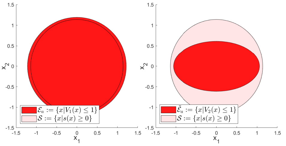
The plots of the ellipsoidal over-approximations $\mathcal{E}_{a}$ and $\bar{\mathcal{E}}_{a}$ of the respective reachable sets $\mathcal{R}_{a}$ and $\tilde{\mathcal{R}}_{a}$ found via the corresponding alternating algorithms and the safe set are given in Fig. 2. It can be seen that, after introducing the secondary controller $h_{s}(x_{2})=-0.31761x_{2}^{3}-1.2534x_{2}$ to the closed loop system, its state $x$ always remains in a subset of the safe set when initialized at the origin.

In this work, based on invariant set analysis and SOS programming, we provide sufficient conditions for safety verification and control design of a class of polynomial nonlinear systems in the presence of adversarial signals. The conditions are computationally tractable via an alternating algorithm. We show that, it is possible to improve the safety performance of a nonlinear system by using a subset of sensors that are attack free. A numerical simulation on a second order nonlinear system verifies the theoretical result.

There are several possible future research direction to be explored. First, it is interesting to investigate a secondary controller design approach that recovers the performance achieved by the primary controller at least locally while ensuring safety. Another interesting topic would be the analysis of how the choice of sensors characterized by the matrix $C_{s}$ impacts the performance of the secondary controller.

References

- [1] A. A. Cárdenas, S. Amin, and S. Sastry, “Research challenges for the security of control systems.,” HotSec, vol. 5, p. 15, 2008.
- [2] Y. Lin, M. S. Chong, and C. Murguia, “Plug-and-play secondary control for safety of LTI systems under attacks,” arXiv preprint arXiv:2212.00593, 2022. To appear in the proceedings of the IFAC World Congress 2023.
- [3] K. Margellos and J. Lygeros, “Hamilton–Jacobi formulation for reach–avoid differential games,” IEEE Transactions on Automatic Control, vol. 56, no. 8, pp. 1849–1861, 2011.
- [4] S. Bansal, M. Chen, S. Herbert, and C. J. Tomlin, “Hamilton-Jacobi reachability: A brief overview and recent advances,” in Proceedings of the IEEE 56th Conference on Decision and Control, pp. 2242–2253, IEEE, 2017.
- [5] F. Blanchini, “Set invariance in control,” Automatica, vol. 35, no. 11, pp. 1747–1767, 1999.
- [6] S. Prajna, A. Jadbabaie, and G. J. Pappas, “A framework for worst-case and stochastic safety verification using barrier certificates,” IEEE Transactions on Automatic Control, vol. 52, no. 8, pp. 1415–1428, 2007.
- [7] A. D. Ames, X. Xu, J. W. Grizzle, and P. Tabuada, “Control barrier function based quadratic programs for safety critical systems,” IEEE Transactions on Automatic Control, vol. 62, no. 8, pp. 3861–3876, 2017.
- [8] S. Coogan and M. Arcak, “A dissipativity approach to safety verification for interconnected systems,” IEEE Transactions on Automatic Control, vol. 60, no. 6, pp. 1722–1727, 2014.
- [9] X. Tan, W. S. Cortez, and D. V. Dimarogonas, “High-order barrier functions: Robustness, safety, and performance-critical control,” IEEE Transactions on Automatic Control, vol. 67, no. 6, pp. 3021–3028, 2021.
- [10] W. Xiao, C. Belta, and C. G. Cassandras, “Adaptive control barrier functions,” IEEE Transactions on Automatic Control, vol. 67, no. 5, pp. 2267–2281, 2021.
- [11] P. Parillo, “Structured semidefinite programs and semialgebraic geometry methods in robustness and optimization,” PhD thesis, California Institute of Technology, 2000.
- [12] Z. Jarvis-Wloszek, R. Feeley, W. Tan, K. Sun, and A. Packard, “Some controls applications of sum of squares programming,” in Proceedings of the IEEE 42nd Conference on Decision and Control, vol. 5, pp. 4676–4681, IEEE, 2003.
- [13] M. Jones and M. M. Peet, “Using SOS and sublevel set volume minimization for estimation of forward reachable sets,” IFAC-PapersOnLine, vol. 52, no. 16, pp. 484–489, 2019.
- [14] A. Teixeira, I. Shames, H. Sandberg, and K. H. Johansson, “A secure control framework for resource-limited adversaries,” Automatica, vol. 51, pp. 135–148, 2015.
- [15] G. Blekherman, P. A. Parrilo, and R. R. Thomas, Semidefinite optimization and convex algebraic geometry. SIAM, 2012.
- [16] S. Boyd, L. El Ghaoui, E. Feron, and V. Balakrishnan, Linear matrix inequalities in system and control theory. SIAM, 1994.
- [17] J. Bochnak, M. Coste, and M.-F. Roy, Géométrie algébrique réelle, vol. 12. Springer Science & Business Media, 1987.
- [18] Z. W. Jarvis-Wloszek, Lyapunov based analysis and controller synthesis for polynomial systems using sum-of-squares optimization. PhD thesis, the University of California, Berkeley, 2003.
- [19] J.-P. Aubin, A. M. Bayen, and P. Saint-Pierre, Viability theory: new directions. Springer Science & Business Media, 2011.
- [20] M. Jones and M. M. Peet, “Using SOS for optimal semialgebraic representation of sets: Finding minimal representations of limit cycles, chaotic attractors and unions,” in Proceedings of the American Control Conference (ACC), pp. 2084–2091, IEEE, 2019.
- [21] H. Yin, M. Arcak, A. Packard, and P. Seiler, “Backward reachability for polynomial systems on a finite horizon,” IEEE Transactions on Automatic Control, vol. 66, no. 12, pp. 6025–6032, 2021.
- [22] K. S. Schweidel, H. Yin, S. W. Smith, and M. Arcak, “Safe-by-design planner–tracker synthesis with a hierarchy of system models,” Annual Reviews in Control, 2022.
- [23] A. Papachristodoulou, J. Anderson, G. Valmorbida, S. Prajna, P. Seiler, P. Parrilo, M. M. Peet, and D. Jagt, “SOSTOOLS version 4.00 sum of squares optimization toolbox for MATLAB,” arXiv preprint arXiv:1310.4716, 2013.
- [24] J. F. Sturm, “Using SeDuMi 1.02, a MATLAB toolbox for optimization over symmetric cones,” Optimization Methods and Software, vol. 11, no. 1-4, pp. 625–653, 1999.