Learning Cellular Coverage from Real Network Configurations using GNNs
Abstract
Cellular coverage quality estimation has been a critical task for self-organized networks. In real-world scenarios, deep-learning-powered coverage quality estimation methods cannot scale up to large areas due to little ground truth can be provided during network design & optimization. In addition, they fall short in producing expressive embeddings to adequately capture the variations of the cells’ configurations. To deal with this challenge, we formulate the task in a graph representation and so that we can apply state-of-the-art graph neural networks, that show exemplary performance. We propose a novel training framework that can both produce quality cell configuration embeddings for estimating multiple KPIs, while we show it is capable of generalising to large (area-wide) scenarios given very few labeled cells. We show that our framework yields comparable accuracy with models that have been trained using massively labeled samples.
Index Terms:
Self-supervised Learning, Graph Neural Network, Cellular Coverage Estimation, Few-shot LearningI Introduction
Estimating mobile users’ Quality of Service (QoS) metrics in cellular networks has been a long-studied problem, in the context of network designing and optimization.
As we approach 6G telecommunication networks, these are expected to be self-aware [1] (i.e., Estimating service QoS-related Key performance indicator (KPI) based on its configurations), paving the way towards the goal of Self-Organized Network (SON).
Estimating radio-coverage-related QoS still remains a challenge, even for cell-level [2] 11
1
We define the term ’cell’ as Evolved Universal Terrestrial Radio Access (eUtran)-Cell, i.e.: the cell’s coverage is denoted by one single carrier frequency’s coverage., mainly due to the complexities that emerge during radio wave propagation. More specifically, to estimate a site with multiple cells’ QoS KPI is NP-hard, whereas it is NP-complete if many sites with heterogeneous inter-cell relations exist.
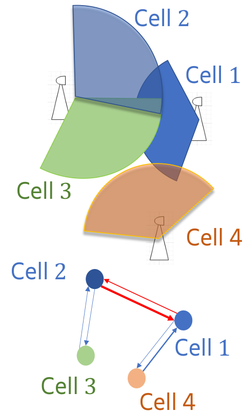
Conventional methods for such problems are often based on logic-based simulations, where the simulator integrates complex radio propagation models and computes the coverage quality on a ‘per-cell’ basis. The simulator, then, integrates the results of each cell to produce the area’s estimation.
Despite the high accuracy of such approaches, these are usually computationally very expensive and in some cases infeasible for cellular coverage computations at scale.
Due to recent advances in deep learning (DL), graph neural networks (GNN) have been proposed as an alternative way to tackle in a time- and computation-efficient way, such computationally difficult sub-problems, such as that of estimating a single cell’s coverage KPI [3, 4], estimating scenarios where a cell holds multiple users [5], as well as estimating multiple cell-user pairs which co-exist in the same scenario [6].
These holistic ‘inter-cell’ relations (illustrated in Fig. 1(a)), though crucial during network design & optimization, need to be learned.
In this paper, we study the KPI estimation problem in the context of a realistic formulation, where we aim to:
A schematic representation of the proposed solution is shown in Fig. 1(b).
Recent DL methods have focused on predicting QoS KPIs of single/multiple cells from the same site, using simulation, crowd-sourcing [7], or road test data (usually collected at a small scale) [8]. However, for cell-level QoS KPI prediction, network measurements are required in both quality and quantity as ground truth. Mobile service providers expect that such a model can:
1. learn from network configurations and their respective measurements in real-world deployments, and 2. scale-up from measurements of a few cells, instead of densely running road measurement tests or frequently triggering measurement reports for the serving users across many cells.On the other hand, properly formulating the QoS KPI estimation task remains an open problem in representation learning, with only few papers [9, 2] adopting representations for modeling ’inter-cell’ relations. Even fewer papers [10] have further considered heterogeneity (e.g: varying inter-site distance) in cells’ representation, which is common in real-world scenarios. A successful formulation of representation would require:
1. great expressivity22 2 The ability of GNN to differentiate small perturbations on node attributes. in terms of cell configuration parameters & ’inter-cell’ relations. 2. the ability to perform well with a limited amount of ground truth/measurements, i.e. as for example in few-shot learning (FSL) settings.Leveraging inter-cell relation with proper representation in a realistic setup using few cells’ network measurements, so far, has not been included in the problem formulation of state-of-the-art studies.
The remaining sections are organized as follows: In Sec. II we discuss the related publications in the domain of QoS KPI estimation of GNNs and DL in the cellular network, while in Sec. III we present our problem formulation in more detail. In Sec. IV we present our methodology followed by Sec. V, which contains the experimental evaluation of our algorithm. Finally, Sec. VI concludes with a discussion of our main contributions and considerations for future work.
II Related Work
Cell configuration parameters are usually devised and fine-tuned by field experts in real-world radio network deployments. Besides the domain knowledge involved in the configuration process, it is considered a laborious task which cannot be easily automated due to the complex relations and interactions between the networks nodes (which is neglected in many previous work [11, 12]). Furthermore, subtle configuration changes may considerably affect the network performance through characteristics such coverage and interference (e.g., cell edge performance [13]). Here, the aim is to produce a model that has learned the associations and relations between cell configuration parameters and their QoS KPI metrics.
Since we need to be able to capture subtle configuration changes, it is essential to employ a representation that has great expressivity. Furthermore, we need to be able to represent heterogeneous data, while learning their relations. GNN satisfies all the above requirements. Our proposed solution models the QoS KPI prediction as a node-attribute prediction task. Many recent advances (e.g.: [14]) in GNNs provide the needed expressivity of the node/edge attributes, which further permits the GNN to learn heterogeneous configuration parameters. On the other hand, graph representations are getting popular in the domain of radio networks. In the context of device-to-device communication, GNNs are used to perform link-level KPI estimation [6, 15, 16]. However, none aforementioned work has addressed ‘inter-cell’ relations with respect to coverage QoS estimation, which poses a cell/system level KPI prediction.
There exist previous studies (e.g., [17]) which address ‘inter-cell’ relations through a graph representation (geo-proximity for the GNN-powered ‘inter-cell’ handover prediction problem). However, these do not consider important aspects such as the heterogeneity of the relations, relations beyond geographically adjacent cells, and spatial orientation of antenna, all of which impact the ‘inter-cell’ relations. Moreover, cellular coverage embeddings have been used together with graph attention to capture the ‘inter-cell’ relations, for the problem of antenna tilt optimization [9]. This is done in a multi-agent reinforcement learning framework, with identical action space for all antennas. However, the authors have not considered few-shot learning, while the results reported cannot be applied to real-world scenarios. In our experiment, we include network configurations crawled from real networks. The data-sets 33 3 Detailed information regarding the dataset, training parameters and respective simulation setup will be presented in Appendix:https://github.com/bluelancer/GNN4NDOSuppliment pose a diverse and unbalanced feature distribution, as each set of configuration parameters is fine-tuned by human experts.
One can consider auxiliary property prediction as a pretext-task in Self-Supervised Learning (SSL) scheme to overcome the data constraint. Formalized by [18], the auxiliary property can incorporate domain knowledge that helps GNN backbone to learn transferable insights. Given such benefit, there exist two open problems:
1. Formulate a proper auxiliary property. 2. Select a suitable training scheme.Some recent works (e.g., [19]) augment auxiliary properties based on embedding’s pairwise similarities. While pre-training (PT) toward such tasks can be generalized as a pre-clustering, such a scheme constrains the expressiveness of the produced embedding.
[20] share a training framework similar to the one we propose, which takes graph generation as pretext-tasks and produces pre-trained embeddings that can be generalized by fine-tuning some ground truth labels. While this method is not suitable for cellular network since:
(i) One can easily determine the interfering/complementing relation by each cell’s carrier so that little supervision can be expected. (ii) This method requires more than 10% of data to be labeled in fine-tuning. This means hundreds of cell measurements, which exceeds the scale of the largest road test dataset to our best knowledge.Beyond the novelty mentioned in Sec. I, we demonstrate the potential for GNN and SSL to be used together in a practical setting: through a novel formulation of auxiliary property inspired by network geometry [21, 22], bringing down the labeling requirement to 2.5%.
III Problem Formulation
We consider the task of estimating the QoS KPI for cell coverage in this paper, which includes two target parameters, Signal to Interference & Noise Ratio (SINR) and Channel Quality Indicator (CQI) for each cell.
- 1.
The ground truth includes a four-dimensional array, denoting the Perfect, Good, Fair and Bad percentage of area, within the cell’s coverage concerning the query KPI.
The input to the problem assumes an attributed directed graph representation that includes:
- 2.
A set of nodes , where each node denotes a cellular coverage.
- 3.
A set of node attributes denoting cells’ configurations, where cell ’s set of configuration is denoted as an array . For -th elements in denotes a configuration parameter (in scalar) .
- 4.
A set of directional edges that connect , denoting the cell relation. Each edge connects from source to destination .
- 5.
A set of edge attributes , denoting the property of ’inter-cell’ relations. For specific edge , the edge’s property is denoted as , pose from source node to destination node . Each includes a three-dimensional array, including a one-hot encoded scalar that denotes the ’inter-cell’ relation type within , a numerical scalar denotes the strength of the relation, and a numerical scalar that denotes geographical distance between and . Knowing the relation is asymmetrical as could interfere with the whole coverage of , while ’s interfering coverage may only take up a small portion of ’s coverage area.
- 6.
A set of measurement features , which are expensive to retrieve as mentioned previously. includes Received Signal Strength Indicator (RSSI) in a four-dimensional array, denoting the Perfect, Good, Fair and Bad percentage of area. is considered as additional node attributes of .
- 7.
A set of augmented geometric features , inspired by recent network geometry studies [21] to model the orientation and shape of the coverage. are considered as additional edge attributes of or a novel pretext-task in a different formulation of the problem. The detailed formulations present as follows.
We consider two problem formulations (PF) in this paper:
- PF1
we include all possible features (i.e. , with abundant ) in training time, to benchmark the upper bound of baseline model performance on estimating .
- PF2
We include only realistic features (i.e. , with few-shot ) in training time, to benchmark and minimize the performance degradation on estimating in FSL.
We report both Transductive and Inductive generalization setting performance in PF1, and report only the Transductive setting performance in PF2. The motivation for a second PF is three-folded:
1. includes RSSI which is not included in signaling from eNB to core network, making this expensive to collect in the real network. 2. A huge amount of ground truth is required for PF1. 3. In Sec. V, we see that the GNN does not learn , which motivates us to use SSL to reinforce the training.A detailed illustration of the problem formulation is provided in Fig. 2
IV Methodology
To prove the argument on GNN’s capability of learning the inter-cell relation for QoS KPI estimation in the above problem formulation, we benchmark many state-of-the-art models that are reported to be leading in coverage QoS KPI estimation task with different expressivity in Sec.II: GAQ/GAT, GINE, WCGCN and multilayer perception (MLP), under different PF with their respective training strategy: GAQ was proposed by [9], on capturing inter-cell relation for antenna tilt optimization with scalability towards unseen size of topology. WCGCN was proposed by [23], for capturing relation between transceiving pairs in D2D communication, for link-level SINR estimation. GINE can be seen as more expressive WCGCN, and is proven to be a suitable backbone for SSL by [23]. MLP is a baseline model that does not incorporate graph structure. In addition, as pointed out by [21], QoS KPIs like SINR strongly depend on each cell’s spatial configuration. We performed an ablation study towards introducing the augmented geometric features as additional node-feature/pretext-task in different PF beyond those included in (i.e., antenna azimuth, sector ID, etc). includes three augmented parameters denoting cell’s spatial configuration, as illustrated in Fig. 3(a) 44 4 We augment globally for all , regardless if and have applied same or different (will not interfere each other in this case) carrier frequency.:
(i) Interference Area (IA): denotes the searching area of possible interference. (ii) Interference Distance (ID): denotes an averaged distance from the interference source in the searching area. (iii) Interference Centric (IC): denotes an averaged location of measurement in the searching area.is augmented based on the horizontal beam-width of the serving antenna, with a radius of 10 55 5 Note: One could use more precise value for estimated coverage radius from crowd-sourcing. Here we used 10 as an upper bound of coverage in cell configuration design. Thus, we guarantee the generalization ability of the solution regardless of the dataset/area..

Besides the performance evaluation, we proposed a novel SSL PT framework for PF2 to tackle the problem with realistic data constrain, as illustrated in Fig. 3(b). Instead of using as input feature, we considered a two-phased training framework:
Phase PT: We consider IA or ID as pretext-task for PT. We first pre-train the selected backbone GNN against the designated pre-text task on edge-level. This selection of pretext-tasks is motivated by a series of work in road test measurement of signal propagation (e.g. [22] points out distance, coordinate and searching areas are key factor to calibrate simulation result to real-world measurement, while IC does not perform well as pretext-task in our experience) Phase FT: We freeze the weight of backbone GNN, and apply newly initialized readout layers on downstream task. Such fine-tuning (FT) formulation is inspired by graph lifelong learning [24]: GNN may able to generalize by taking over the knowledge gained in related previous tasks, even few ground truth is provided in downstream tasks.In Phase PT, given the ground truth of select pretext-task being , we introduce the loss function in Equ. 1:
| (1) |
where denotes the number of edges in the training data. denotes the output node embedding after readout layers , for node , respectively. In Phase FT, we adopt mean squared error (MSE) as loss function for downstream task ground truth . We denote as the percentage required for labeled data in Phase FT. To summarize, we present the pseudo-code in Algorithm 1. Note represents concatenating model weight dict and .
- 1.
Epoch length: ,; percentage of ground truth needed: ; training hyper-parameter for Phase PT and FT: ,.
- 2.
Backbone model , weight ; PT readout layers , weight ; and downstream readout layers , weight .
- 3.
Prepare graph representation , pretext-task ground truth for all . Uniformly sample by . Prepare downstream task ground truth . Optimizer .
- 4.
- 5.
- 6.
Frozen .
- 7.
- 8.
Select ’s embeddings from
- 9.
V Experiment
We have trained our model against the real network configuration in two geographical locations, i.e., Copenhagen (CPH) and Aalborg-Aarhus (A+A).
The network measurement and KPIs are obtained from simulation in Info-Vista Planet 3.
PF1: We first benchmark the state-of-the-art performance of GNNs benchmark in the Transductive setting, with an ablation study against as an additional node feature. The result in is presented in Table I. For the generalization setting, we denote as training on dataset and test the model performance on dataset to verify the model’s generalization ability across different scenarios. Similarly, the generalization performance is shown in Table II.
| Model | KPI | CPH | CPH(w.) | A+A | A+A(w.) |
| GAT | SINR | 5.7 ± 0.5% | 5.6 ± 0.5% | 5.6 ± 0.2% | 5.6 ± 0.1% |
| WCGCN | SINR | 3.2 ± 0.7% | 3.1 ± 0.3% | 1.1 ± 0.1% | 1.1 ± 0.2% |
| GINE | SINR | 3.4 ± 0.3% | 3.5 ± 0.4% | 2.0 ± 0.1% | 1.8 ± 0.2% |
| MLP | SINR | 5.5 ± 0.1% | 5.5 ± 0.1% | 5.5 ± 0.1% | 5.5 ± 0.1% |
| GAT | CQI | 0.31 ± 0.1% | 0.30 ± 0.1% | 2.9 ± 0.1% | 2.9 ± 0.1% |
| WCGCN | CQI | 0.24 ± 0.2% | 0.24 ± 0.1% | 1.3 ± 0.2% | 1.2 ± 0.2% |
| GINE | CQI | 0.28 ± 0.2% | 0.26± 0.1% | 1.7 ± 0.1% | 1.6 ± 0.2% |
| MLP | CQI | 0.3 ± 0.1% | 0.29 ± 0.1% | 3.1 ± 0.1% | 3.1 ± 0.1% |
| Model | KPI | CPHA+A | CPHA+A(w.) | A+ACPH | A+ACPH(w.) |
|---|---|---|---|---|---|
| GAT | SINR | 9.2 ± 0.2% | 9.35 ± 0.3% | 11.3 ± 0.8% | 11.2 ± 0.7% |
| WCGCN | SINR | 9.5 ± 0.3% | 9.4 ± 1.7% | 11.6 ± 0.3% | 8.7 ± 0.3% |
| GINE | SINR | 9.4 ± 2.0% | 11.5 ± 4.2% | 12.3 ± 3.0% | 8.7 ± 0.2% |
| MLP | SINR | 12.0 ± 0.2% | 12.1 ± 0.9% | 10.9 ± 0.7% | 10.9 ± 0.7% |
| GAT | CQI | 3.7 ± 0.2% | 3.5 ± 0.8% | 0.39 ± 0.1% | 0.45 ± 0.7% |
| WCGCN | CQI | 4.3 ± 0.1% | 4.05 ± 0.0% | 0.34 ± 0.2% | 0.52 ± 0.3% |
| GINE | CQI | 3.8 ± 0.7% | 4.9 ± 2.9% | 0.52 ± 0.4% | 1.13 ± 0.9% |
| MLP | CQI | 3.5 ± 0.4% | 3.5 ± 0.4% | 0.88 ± 0.4% | 0.88 ± 0.4% |
Given presented result in Tables I and II, one can conclude that,
• For Table I: (i) WCGCN outperforms most benchmark models when given sufficient measurement on QoS KPI, while GAT has almost equivalent performance to MLP, which is aligned with the conclusion of [9]. (ii) Comparing the performance between ‘with’ and ‘without’ as additional edge attribute in Table I, we observe that the augmented geometric feature does not improve transductive performance with sufficient ground truth. (iii) Comparing the respective cells between Table I and II, we observe that the GNN model can not generalize its performance to new area/dataset, without degradation. This is aligned with the conclusion of Appendix A by [25], as the test dataset introduces unseen structural feature and graph size during training time. (iv) By carefully studying the variance (e.g: GINE on CPHA+A) on the in Table II, we find that weight initialization in training time has a dominant impact on the inductive generalization performance toward another dataset. (v) Seeing Table II, introducing geometric feature (w. columns) does not benefit GNN generalization performance stably.PF2: Since PF1 conclude that given sufficient measurement on QoS KPI, the network geometric could be less important for GNNs. We further studied the importance of in a realistic PF. In PF2, we compared our proposed SSL framework with state-of-the-art training framework, as Fig. 1(b). We adjust provided percentage of ground truth to verify the gain brought by Phase PT in SSL.
In Table III, we consider two different baselines:
1. We consider no PT training scheme as a first baseline: if we applied a successful pretext-task, the GNN performance should outperform the same model without PT. We list the performance diff in column Gain. Green text denotes SSL result (i.e. ID/IA) outperform the benchmark by a positive gain (i.e. ), while Red text denotes a negative gain, indicating introducing pretext-task has down-graded performance. 2. We consider MLP as a second baseline: Given MLP does not incorporate inter-cell relation, if any GNN model benefits from SSL more than MLP does with the same (e.g: ), we consider the SSL framework is helping GNN backbone to incorporate inter-cell relation better, and color the block in green.Given the presented result in Table III, one can conclude:
(i) GNN degrades heavily with insufficient ground truth compared with PF1. When compared with the second baseline (MLP), one can see degradation is not only due to difficulty in generalizing towards inter-cell relational features but also node attributes, as MLP also improves its SSL performance for CQI task. (ii) When compared with the first baseline (train without SSL), SSL PT benefits GNNs unevenly on both inter-cell relational feature and node attributes. (iii) For the QoS KPI estimation task, a more expressive GNN backbone benefits more from PT, than less expressive ones (e.g., GINE is considered to be expressive by [23], while WCGCN is less expressive due to an additional maxpool during message passing beyond GINE’s design [6], expressiveness: GINE WCGCN GAT). This is aligned with the conclusion by [23] who observed similar behavior in chemistry & biology datasets. However, their solution is limited to small, non-planar graphs while our work extends the conclusion for QoS KPI estimation, where the graph is near-planar. Furthermore, we cherry-pick the best-performing model in FSL by dataset and their estimating KPI to compare against the same model’s performance in full training in table IV, where ’SOTA’ denotes a full training using 80% of ground truth (aligned with Fig. 3(b), State-of-the-art training scheme). This supports our augments that a proper SSL framework with only 2.5% ground truth can compete with ’SOTA’ training in many downstream tasks.We consider that our pre-text task (IA/ID) helps our GNN models to learn network geometry knowledge, which enables them to outperform the state-of-the-art training framework. Finally, we include a comparative result in table V between GNN solution and the baseline simulator InfoVista Planet to prove GNN is more time and computationally efficient. Seeing from the RAM and inference time, GNN is significantly superior to the baseline simulator. Since inference time for GNN is cell-independent, we exclude the running time for the simulator for preprocessing per-cell’s configuration parameter as that can grow linearly with the number of cells for a fair comparison. (This step could take additional 2 hours for an A+A dataset.) One can also see from search space size: In dataset (A+A) with more rural components, each cell’s QoS estimation is less dependent on its neighboring cell than the ’more urban’ one (CPH). Both methods reflect that, while GNN more aggressively reduces the search space, this accelerates its inference, but degrades its performance in more urban areas.
| Model | GNN (GINE/WCGCN) | InfoVista Planet | ||
| Dataset | CPH | A+A | CPH | A+A |
| RAM | MiB | MiB | GiB | GiB |
| Inference Runtime | 13.18 min | 36.72 min | ||
| Searchspace per result | ||||
VI Conclusion
The paper evaluates state-of-the-art coverage-estimation-targeted GNNs in real-world configurations and identifies inefficiencies in generalization when transferring learning outcomes from one scenario to another. In addition, we formulate a more realistic few-shot learning problem that considers data constraints and propose a novel pretext-task for PT to facilitate FSL performance with minimal performance degradation. Our training framework confirms the benefits of SSL with fewer ground truth samples. Future work can focus on improving the model’s generalization ability and exploring additional zero-shot estimation schemes.
Acknowledgement
This work was partially supported by the Wallenberg AI, Autonomous Systems and Software Program (WASP) funded by the Knut and Alice Wallenberg Foundation.
References
- [1] Abdelaali Chaoub et al. “Self-Organizing Networks in the 6G Era: State-of-the-Art, Opportunities, Challenges, and Future Trends” In IEEE Communications Standards Magazine, 2022
- [2] Eren Balevi and Jeffrey Andrews “Online antenna tuning in heterogeneous cellular networks with deep reinforcement learning” In IEEE Transactions on Cognitive Communications and Networking 5.4 IEEE, 2019, pp. 1113–1124
- [3] Jakob Thrane, Benjamin Sliwa, Christian Wietfeld and Henrik Christiansen “Deep learning-based signal strength prediction using geographical images and expert knowledge” In IEEE GLOBECOM, 2020, pp. 1–6 IEEE
- [4] Wei Cui, Kaiming Shen and Wei Yu “Spatial deep learning for wireless scheduling” In IEEE JSAC 37.6 IEEE, 2019, pp. 1248–1261
- [5] Nuwanthika Rajapaksha, KB Manosha, Nandana Rajatheva and Matti Latva-Aho “Deep learning-based power control for cell-free massive MIMO networks” In ICC, 2021, pp. 1–7 IEEE
- [6] Yifei Shen, Yuanming Shi, Jun Zhang and Khaled Letaief “Graph neural networks for scalable radio resource management: Architecture design and theoretical analysis” In IEEE JSAC 39.1 IEEE, 2020, pp. 101–115
- [7] Andrea Pimpinella, Andrea Marabita and Alessandro Redondi “Crowdsourcing or network kpis? A twofold perspective for QoE prediction in cellular networks” In WCNC, 2021, pp. 1–6 IEEE
- [8] Arvind Narayanan et al. “Lumos5G: Mapping and predicting commercial mmWave 5G throughput” In Proceedings of the ACM Internet Measurement Conference, 2020, pp. 176–193
- [9] Yifei Jin et al. “A graph attention learning approach to antenna tilt optimization” In 6GNet, 2022, pp. 1–5 IEEE
- [10] Ryan Dreifuerst et al. “Optimizing coverage and capacity in cellular networks using machine learning” In IEEE ICASSP, 2021, pp. 8138–8142 IEEE
- [11] Aristotelis Margaris, Ioannis Filippas and Kostas Tsagkaris “Hybrid Network–Spatial Clustering for Optimizing 5G Mobile Networks” In Applied Sciences 12.3 MDPI, 2022, pp. 1203
- [12] Aliye“”Ozge Kaya and Harish Viswanathan “Deep Learning-based predictive beam management for 5G mmwave systems” In WCNC, 2021, pp. 1–7 IEEE
- [13] Xiaohu You, Dongming Wang, Pengcheng Zhu and Bin Sheng “Cell Edge Performance of Cellular Mobile Systems” In IEEE JSAC 6.29, 2011, pp. 1139–1150
- [14] Keyulu Xu, Weihua Hu, Jure Leskovec and Stefanie Jegelka “How Powerful are Graph Neural Networks?” In ICLR, 2019
- [15] Xiaochen Zhang et al. “Scalable Power Control/Beamforming in Heterogeneous Wireless Networks with Graph Neural Networks” In IEEE GLOBECOM, 2021
- [16] Yifei Shen, Jun Zhang, SH Song and Khaled Letaief “Graph Neural Networks for Wireless Communications: From Theory to Practice” In IEEE Transactions on Wireless Communications, 2022
- [17] Zi Wang et al. “Spatial-Temporal Cellular Traffic Prediction for 5 G and Beyond: A Graph Neural Networks-Based Approach” In IEEE Transactions on Industrial Informatics IEEE, 2022
- [18] Yixin Liu et al. “Graph self-supervised learning: A survey” In TKDE IEEE, 2022
- [19] Wei Jin et al. “Node similarity preserving graph convolutional networks” In ACM WSDM, 2021, pp. 148–156
- [20] Ziniu Hu et al. “Gpt-gnn: Generative pre-training of graph neural networks” In SIGKDD, 2020, pp. 1857–1867
- [21] Chunlin Chen “Stochastic geometry modeling and performance evaluation of cellular networks”, 2018
- [22] Seong-Yun Cho “Simultaneous LTE Signal Propagation Modelling and Base Station Positioning Based on Multiple Virtual Locations” In Sensors 22.15 MDPI, 2022, pp. 5917
- [23] W Hu et al. “Strategies For Pre-training Graph Neural Networks” In ICLR, 2020
- [24] Lukas Galke, Benedikt Franke, Tobias Zielke and Ansgar Scherp “Lifelong learning of graph neural networks for open-world node classification” In IJCNN, 2021, pp. 1–8 IEEE
- [25] Gilad Yehudai et al. “From local structures to size generalization in graph neural networks” In ICML, 2021, pp. 11975–11986 PMLR