MATOQ: a Monte Carlo Simulation of Electron Transport in Environmental-friendly Gas Mixtures for Resistive Plate Chambers
Abstract
The increasing interest in environmentally friendly gas mixtures for gaseous particle detectors, especially tetrafluoropropene-based gas mixtures for Resistive Plate Chambers (RPCs), has prompted the need for simulating electron transport coefficients and reaction rates in these mixtures in recent years. MATOQ is a Monte Carlo simulation program that calculates electron transport parameters, specifically designed for studying and optimizing environmental-friendly gas mixtures for RPCs. Unlike other existing codes, MATOQ allows for the simulation of electron avalanches by including the effect of space charge electric field, which can significantly impact the avalanche evolution in gaseous detectors such as RPCs.
After the validation of the MATOQ simulation in the temporal and spatial growth configurations, we present the electron transport coefficients and the reaction rates in tetrafluoropropene-based gas mixtures, which may represent a valid alternative to the standard gas mixtures currently used for RPCs.
I Introduction
Resistive Plate Chambers (RPCs) are gaseous particle detectors used in high-energy physics experiments Santonico and Cardarelli 1981; Bruno 2004; Abbrescia et al. 2012; Zeballos et al. 1996a and medical imaging applications Amaldi et al. 2015; Crespo et al. 2013. They consist of two parallel plates made of high-resistivity materials with a gap between them filled with a gas mixture. Tetrafluoroethane (C2H2F4) is generally the main component of the gas mixtures for RPCs. This gas is typically mixed with quench gases such as isobutane (i-C4H10) and sulfur hexafluoride (SF6) in various proportions to optimize the performance of RPCs for specific applications.
In view of supporting the transition to a green economy and fighting climate change, recent regulations of the European Union have prohibited the use of C2H2F4 for many applications, since it is a greenhouse gas. Indeed, the global warming potential of C2H2F4 is about 1430 Intergovernmental Panel on Climate Change (2014) IPCC. This means that the impact of this gas on the greenhouse effect is estimated to be 1430 times higher than an equivalent mass of carbon dioxide (CO2) in the atmosphere. Although there are no European regulations restricting the use of C2H2F4 for scientific applications, some research teams Abbrescia et al. 2016a; Guida et al. 2016; Liberti et al. 2016; Bianchi et al. 2019 have explored the possibility of replacing C2H2F4 with more environmentally friendly gases. Many experimental studies are currently focused on measuring the performance of RPCs by replacing the current C2H2F4-based gas mixture with environmental-friendly alternatives Bianchi et al. 2019; Proto et al. 2022; Abbrescia et al. 2016b; Rigoletti et al. 2020. Recently, some encouraging results have been obtained by replacing the C2H2F4 with tetrafluoropropene. Tetrafluoropropene (C3H2F4) has a chemical composition similar to C2H2F4, but it seems much more electronegative than C2H2F4 Chachereau et al. 2016; Bianchi et al. 2020. This would result in too high operating voltages for RPCs that are not compatible with the already existing power supply systems. Instead of replacing C2H2F4 with only C3H2F4, binary mixtures of C3H2F4 and CO2 may be a feasible alternative Bianchi et al. 2019; Proto et al. 2022; Abbrescia et al. 2016b; Rigoletti et al. 2020. However, purely experimental studies require a large number of trials to identify gas mixtures that yield satisfactory performance of RPCs.
The simulation of electron transport coefficients and reaction rates under the influence of the electric field can assist in the selection of the most promising eco-friendly gas mixtures for RPCs. In recent years, some Monte Carlo programs to simulate electron transport in gases under the influence of a static and uniform electric field have been developed for specific applications. One of the most widely used codes is MAGBOLTZ that was developed by S. Biagi in the 1990s and has been regularly updated Biagi 1999. This open-source code, written in FORTRAN, is still used in the field of gaseous particle detectors. However, one of the most significant limitations is that the input electron collision cross sections for all gases are deeply embedded in the MAGBOLTZ code. This makes it challenging to implement new sets of electron collision cross sections, like those for C3H2F4 Bianchi et al. 2021, and modifying the code for specific purposes can be complicated. Some attempts have been recently done to implement more user-friendly Monte Carlo simulations similar to MAGBOLTZ. In particular, the METHES program Rabie and Franck 2016 overcomes the limitation of MAGBOLTZ in simulating electron transport in gases not yet included in the internal database. Indeed, different sets of electron collision cross sections can be easily adopted as input in METHES. However, the execution of METHES requires a commercial license of MATLAB Rabie and Franck 2016. In addition, it is important to note that MAGBOLTZ and METHES do not account for the effect of the space charge electric field, which can significantly impact the avalanche evolution, especially in RPCs with narrow gas gaps.
This paper describes the MATOQ program that is a Monte Carlo simulation focused on the calculation of electron transport coefficients and reaction rates in any gas mixture of interest under the influence of the electric field. This is obtained by simulating the temporal and spatial growth of electron avalanches along gas gaps. In addition, MATOQ allows simulating the electron avalanche growth under the influence of a static applied electric field together with the space charge electric field that changes depending on the avalanche evolution along a given gas gap. This aspect sets the MATOQ program apart from all other available Monte Carlo simulations.
MATOQ is implemented in the programming language C++, which facilitates its usage and customization in various research fields where C++ is commonly used, such as in the simulation of gaseous particle detectors. MATOQ is compatible with the file format of electron collision cross sections adopted by the open-access Plasma Data Exchange Project (LXCat) Pancheshnyi et al. 2012 in order to allow the user to easily control all input parameters. Moreover, MATOQ is interfaced with OpenMP Dagum and Menon 1998 to enable multi-thread execution, and with the ROOT program Antcheva et al. 2011 for the graphical representation of simulation results.
The paper is organized as follows. In section II we describe how the space charge electric field may play a significant role in the electron avalanche growth. The methodology to simulate the electron transport in gases is presented in section III, while the simulation of collisions between electrons and neutral gas molecules is examined in section IV. Sections V and VI describe the temporal and spatial growth configurations of MATOQ, whereas the simulation of the avalanche growth under the influence of the applied electric field together with the space charge electric field is detailed in section VII. In section VIII, we compare the electron transport coefficients and reaction rates in pure C2H2F4, pure C3H2F4, and in binary mixtures of C3H2F4 and CO2. Furthermore, we describe how the avalanche size in a narrow-gap RPC is affected when C2H2F4 is substituted by C3H2F4. Finally, conclusions are drawn in section IX.
II Space charge electric field
Free charged particles gain energy in gases under the influence of an electric field. Since the ion mobility is generally three orders of magnitude lower than that of electrons Abbrescia et al. 2018, the velocity of ions in gases is generally negligible in comparison to that acquired by electrons. As a result, the number of electrons grows exponentially by giving rise to an electron avalanche. Indeed, under the influence of the electric field, electrons can gain enough energy to ionize a certain number of gas molecules along their drift towards the anode. On the contrary, ions generally drift towards the cathode without playing a fundamental role in the charge multiplication due to their low energy. In this work, the motion of ions is not simulated since they move much slower than electrons. Nevertheless, the motion of ions can be easily implemented in MATOQ by including the ion mobility of each species in the gas mixture of interest.
During the avalanche growth in gases, electrons and ions are partially overlapped in space while they move towards the opposite electrodes. This generates an electric field, generally called space charge electric field, that is superimposed on the applied electric field. As a consequence, the applied electric field turns out to be reduced in the middle of the electron avalanche because it is lowered by the space charge electric field between electrons and ions. On the contrary, the applied electric field is strengthened in the upstream and downstream avalanche as it is reinforced by the space charge electric field. This causes a non-uniform electric field during the avalanche evolution in gas gap that depends on free charges and their positions in time. One of the common devices where space charge effects can have a significant impact is gaseous particle detectors, in particular narrow-gap RPCs. Abbrescia et al. 2018; Zeballos et al. 1996b.
MATOQ allows for calculating or excluding space charge effects in simulations depending on the desired outcome. In sections V and VI, the space charge electric field is not assessed in order to validate the MATOQ calculations with the results of MAGBOLTZ, in which the space charge effects cannot be simulated. On the contrary, in section VII, the space charge electric field is considered for simulating the average avalanche size as a function of the applied electric field in an RPC with a gas gap of 0.1 mm. This is done to enable a comparison between the MATOQ results and those obtained by the Lippmann et al.’s model, which can be used to calculate the electron avalanche size in RPCs Lippmann and Riegler 2004.
III Methods
The MATOQ simulation program tracks the motion of electrons for the entire duration of the simulation, while ions are considered motionless during electron avalanche development due to their much lower mobility compared to electrons. The position and the velocity of a free electron in a gas mixture under the influence of the applied electric field is determined according to the following equations:
| (1) |
where is the time step of the simulation, while and are the electron mass and charge, respectively. The kinetic energy of an electron with velocity is given by:
| (2) |
The choice of an appropriate time step to perform the MATOQ simulation is determined by the null-collision technique Skullerud 1968; Koura 1986. According to this technique, the probability of time steps higher than is:
| (3) |
where is the time and is the collision frequency, which depends on the electron velocity . Indeed, the collision frequency can be expressed as:
| (4) |
where denotes the number of gas molecules per unit volume, which is assumed constant in space and time in all MATOQ simulations, and is the cross section of each individual process that can take place in the gas mixture. For a gas mixture consisting of components with respective concentrations , the total cross section is given by:
| (5) |
where is the index of each gas component, while the index , ranging from 1 to , corresponds to each individual electron collision process that can occur in the gas component . Using the null-collision technique, a constant trial collision frequency () is introduced and assumed higher than the total collision frequency in the whole energy range of interest. As a consequence, the expression of is:
| (6) |
The total cross section is evaluated in MATOQ between 0 eV and 100 eV, whereas the trial collision frequency is assumed three times higher than . As a result, the introduction of a constant trial collision frequency that is independent of the electron velocity gives the possibility to recast the probability as follows:
| (7) |
Therefore, the selection of the time step can be determined by the generation of a random number. Using the inverse transformation method for the distribution , the time step is calculated as follows:
| (8) |
where is a random number generated from a uniform distribution in the range (0, 1].
For each electron, identified by the index , the possibility that a real collision may occur is checked after every time step . The number of all possible processes at the corresponding velocity is determined to define a vector with +1 items for each electron Rabie and Franck 2016. Subsequently, the single item of the vector is initialized as:
| (9) |
where is the occurrence probability of -th electron collision process. According to equation 9, the content of each item is cumulatively summed to obtain an integral function that monotonically increases. Since a null-collision can occur, the total number of items in the vector is +1 and each collision frequency is normalized by , which is higher than the total collision frequency , in accordance with the equation 6. By means of this normalization, the last item of the vector represents the occurrence probability of a null-collision, in which no real collision occurs.
IV Types of electron collisions
For each type of electron collision, MATOQ needs the corresponding cross section as a function of the incident electron energy as input. Since there are different sets of electron collision cross sections present in the literature for the most common gases, MATOQ is compatible with the data format used in the LXCat database, which includes a vast collection of sets for various gases Pancheshnyi et al. 2012. This is the same approach adopted in METHES, whereas MAGBOLTZ utilizes a database included in the code and updated and reviewed periodically by its developer.
In MATOQ, simulations of electron-neutral gas molecule collisions are carried out, while interactions between electrons and between electrons and ions are not considered. The possible electron collisions that can be simulated include: (a) elastic processes, where the interaction involves an electron and a neutral gas molecule in both the initial and final states; (b) excitations, where an incident electron transfers part of its energy to a neutral gas molecule, promoting it to an excited state. However, secondary effects such as photon emission are not considered in MATOQ; (c) ionization and attachment events, where an incident electron ionizes a neutral gas molecule or is captured by it, respectively.
In the LXCat database, cross sections for every type of electron collision are presented as tables of values that vary as a function of the incident electron energy. In MATOQ, each cross section value is linearly interpolated with the subsequent value in the table to obtain a continuous function that spans the entire energy range of interest.
In order to select the type of electron collision to simulate in MATOQ, a random number is generated from a uniform distribution ranging from 0 to 1 for each time step . If is smaller than the content of in equation 9, the first collision process is simulated. If is larger than the (-1)-th item and smaller than the -th item, the -th process is simulated. If is higher than the content of , a null-collision is selected, which means that the electron continues its free motion without any interactions with the gas medium Rabie and Franck 2016.
In the case of elastic collisions, isotropic scattering is assumed in the simulation, meaning that the polar angle and the azimuthal angle are determined as follows Rabie and Franck 2016:
| (10) |
where and are random numbers generated from a uniform distribution ranging from 0 to 1. In addition to the simulation of the resulting electron trajectory, it is necessary to evaluate the energy loss of the incident electron for each elastic collision. Since gas molecules are assumed to rest in the laboratory system for simplicity, the energy loss of the incident electron after the elastic scattering with the neutral gas molecule of mass is given by Rabie and Franck 2016; Landau and Lifshitz 2013:
| (11) |
where is the incident electron energy, is the electron mass and is given by the equation 10. On the contrary, the electron energy loss after an excitation or ionization process is given by:
| (12) |
where is the energy threshold of the specific event to simulate. In other terms, the incident electron energy is assumed to be reduced by the minimum energy required to excite or ionize the gas molecule, depending on the type of process simulated. The scattering of the incident electron in excitation and ionization processes is considered isotropic as in the case of elastic processes. The values of used in MATOQ are obtained from the LXCat database along with the electron collision cross sections. More details on simulating ionization and attachment processes are given in sections V and VI, depending on the chosen temporal or spatial growth configuration. In the case of a null-collision, the electron does not interact with the gas medium and continues its motion.
V Temporal growth configuration
In the temporal growth configuration of MATOQ, trajectories and collisions of an ensemble of electrons are simulated in an infinite gas volume. The number of electrons remains constant for the entire duration of the simulation. This configuration enables the determination of various electron properties such as their mean energy, drift velocity, and ionization and attachment coefficients.
MATOQ implements the same technique used in METHES Rabie and Franck 2016 to maintain a constant number of electrons at every time step . In the case of an ionization event, an additional electron is added to the electron ensemble, while a different electron is randomly removed. The new electron is simulated from the initial position where the ionization occurred. The remaining electron energy, calculated as the difference between the energy of the incident electron and the ionization energy of the involved gas molecule (according to equation 12), is equally shared between the two electrons resulting from the ionization collision. On the contrary, in the case of attachment processes, the attached electron is removed from the electron ensemble, and an additional electron is added to the same position where the attachment event occurred. The direction and energy of the new electron are assumed to be the same as those of an electron randomly selected from the ensemble.
The reliable calculation of electron transport coefficients and reaction rates is only possible after the electron ensemble has reached a steady state regime, where the mean electron energy remains constant, except for statistical fluctuations. All electrons in the MATOQ simulation start with an initial energy of 0.1 eV. Figure 1 shows the time evolution of the mean energy of 105 electrons in pure argon (Ar) at a reduced electric field of 150 Td11 1 1 Td = 10-21 Vm2. After approximately 10-11 s, the mean electron energy reaches a constant value of around 7 eV, with small statistical variations (0.5 eV).
The instantaneous mean electron energy at the time is given by:
| (13) |
where indicates the -th electron with velocity , whereas is the total number of electrons. Similarly to the calculation of the instantaneous mean electron energy, the instantaneous mean electron velocity at the time is given by:
| (14) |
Since the number of electrons does not change in the temporal growth configuration of MATOQ, the number of ionizations and attachments increases linearly in time Rabie and Franck 2016. Therefore, the ionization () and electron attachment () coefficients at the time are given by:
| (15) |
where and are the number of the ionizations and electron attachments at the time instant , respectively, whereas and correspond to the number of ionization and attachment events at time instant with .
To accurately evaluate all electron transport coefficients and reaction rates, the electron ensemble must reach a steady state. Therefore, , , and are only calculated after this condition has been met. The mean electron energy and the mean electron velocity are determined in MATOQ by averaging all respective values of and , sampled at each time step after reaching the steady state. In this work, the drift velocity is defined as the component of velocity along the direction of the applied electric field . The ionization and attachment rates, and , are calculated by counting the respective processes every 1000 time steps after reaching the steady state. This ensures that enough ionization and attachment events occur between samplings. The values of , , and are subject to statistical fluctuations, and their uncertainties are estimated by computing the standard deviation of the corresponding values obtained at each sampling.
The temporal growth configuration in MATOQ simulation ends after a specified number of real collisions, which is selected by the user. Increasing the number of real collisions improves the accuracy of results in Monte Carlo simulations, but it also increases the computation time Biagi 1999; Rabie and Franck 2016. In MATOQ, tens of millions of real collisions generally result in a reasonable computation time with satisfactory accuracy.
To validate the MATOQ simulation, we compare the calculated values of , , , and as a function of the reduced electric field with MAGBOLTZ results in both pure Ar and nitrogen (N2) gases. Additionally, we examine the accuracy of MATOQ by comparing the results with MAGBOLTZ in a binary mixture of 50% Ar and 50% N2 as well as in pure CO2 where electron attachments can occur, unlike in Ar and N2. The electric field is assumed uniform in the gas medium in all these cases. No space charge effects are considered here. Figure 2 shows values of , , and as a function of in pure Ar, N2, CO2 and in the gas mixture composed of 50% Ar and 50% N2. For each value of , MATOQ simulation results are obtained with 105 electrons and the maximum number of real collisions is set equal to 4108 as in MAGBOLTZ. The steady state is assumed to be reached in MATOQ after 1108 real collisions. Sets of electron collision cross sections used for simulations are specified in the appendix.
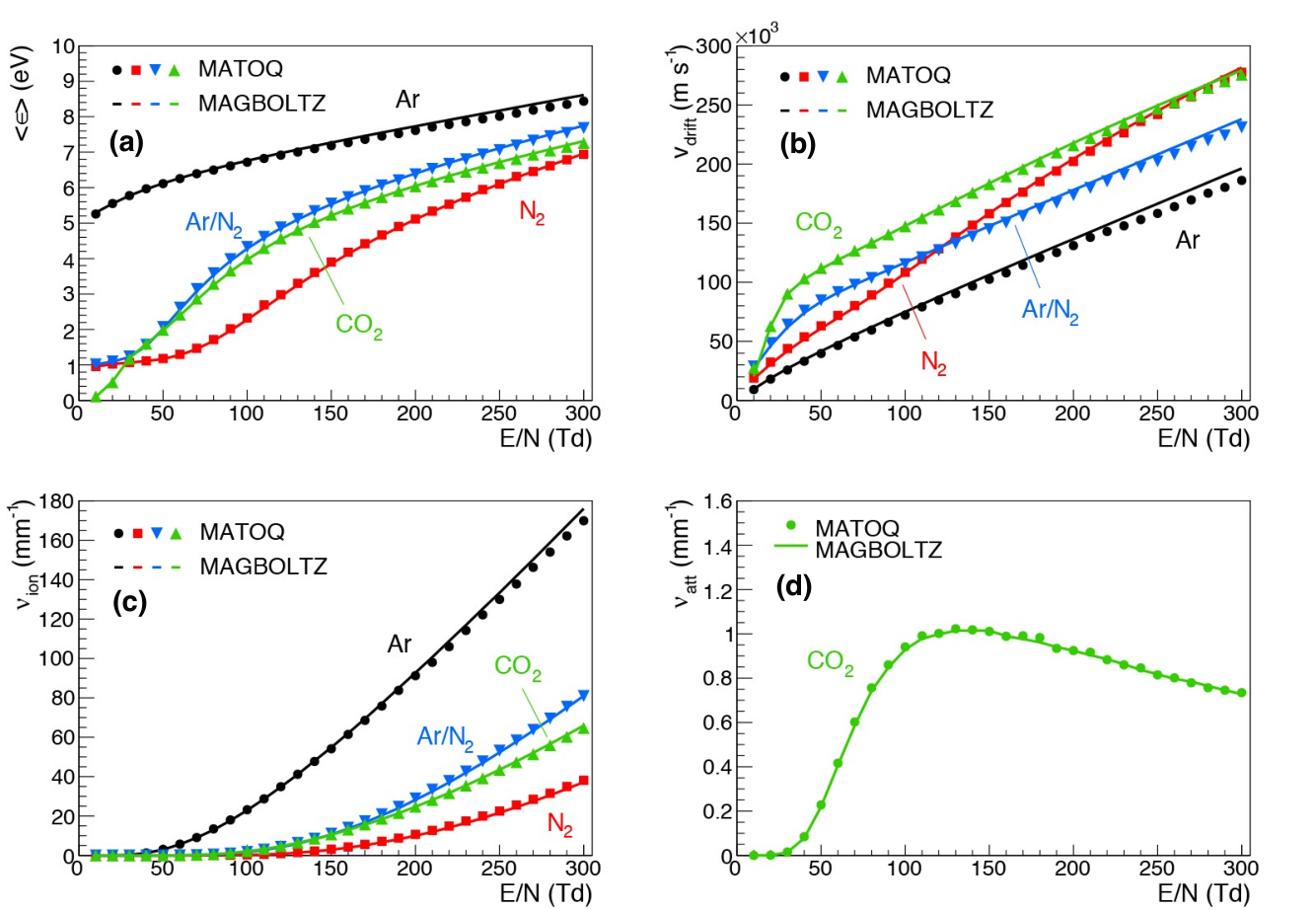
The comparison between MATOQ and MAGBOLTZ calculations in all four gas mixtures shows a good agreement, as displayed in figure 2. The relative error22 2 The relative error of the generic parameter is defined in percentage as follows: (16) where AMQ() and AMZ() are the values of the parameter () calculated at the value with MATOQ and MAGBOLTZ, respectively. in the values of , , and is below 1% for all gas mixtures tested, except for pure Ar at values above 200 Td, where the relative error increases up to about 5%. This discrepancy is likely due to the assumption in MATOQ that the energy resulting from ionization collisions is equally shared between the two electrons in the final state, which may lead to less accurate results compared to MAGBOLTZ. This effect is more pronounced in Ar at higher values where ionization events are more frequent compared to the other gases.
VI Spatial growth configuration
The spatial growth configuration simulates an electron avalanche in an infinite gas volume, with a certain number of initial electrons and a given value. The number of electrons is not fixed during the simulation. An additional electron is added to the avalanche upon ionization, while the trajectory of an electron is not simulated anymore when it becomes captured by a gas molecule. This configuration allows us to determine the ionization () and attachment () Townsend coefficients. In the presence of ionization and attachment processes, the number of electrons at the distance is given by:
| (17) |
where is the initial number of electrons while and are the ionization and attachment Townsend coefficients, respectively. The difference between and is usually named effective ionization Townsend coefficient .
The spatial growth configuration of MATOQ simulates the electron transport and energy transfer after collisions in the same way as the temporal growth configuration, with the exception of ionization and attachment processes. Upon ionization, an additional electron with a random initial direction is added to the simulation, and the two electrons resulting from the collision share the remaining energy equally. The trajectory of the new electron starts from the same position as the incident electron. In the case an electron becomes attached to a gas molecule, its motion is not simulated any further. It should be noted that the spatial growth configuration may not be effective in the presence of high attachment coefficients, as all electrons in the avalanche could become attached before the simulation concludes.
The evaluation of and for a given value in MATOQ is performed by counting the number of electrons that cross a series of virtual planes, placed at the same distance apart and perpendicular to the electric field direction. The position of the virtual planes is determined based on the positions of the slower electron at the beginning of the steady state and at the end of the simulation. To obtain reliable values of and , tens of virtual planes are usually sufficient. During the simulation, the initial and final position of each electron is recorded, and the number of electrons crossing each virtual plane is counted. Interpolation of the number of electrons as a function of virtual plane position with an exponential function allows for the calculation of the effective ionization Townsend coefficient, , using equation 17. To obtain , the interpolation is repeated without accounting for attachment processes. Finally, is calculated as the difference between and . Uncertainties of and are assumed to be equal to the uncertainties of the corresponding best-fit functions on simulation data, and error propagation is used to determine the uncertainty of .
The instantaneous mean electron energy and the instantaneous velocity of electrons in the avalanche are evaluated by implementing equations 13 and 14 where is here the number of electrons simulated at time . Similarly to the temporal growth configuration, the mean electron energy and the electron velocity are calculated in MATOQ by averaging all respective values sampled at each time step after reaching the steady state.
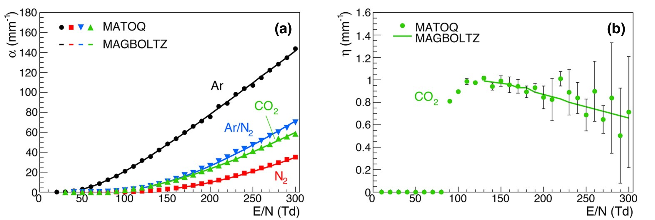
The validation of the spatial growth configuration of MATOQ is done by comparing the calculated values of and as a function of with those obtained from MAGBOLTZ calculations in pure Ar, N2, CO2, and in the gas mixture of 50% Ar and 50% N2. In the spatial growth configuration of MATOQ, the simulation ends after either reaching 1108 real collisions or simulating a maximum number of 106 electrons, whichever comes first. The steady state is assumed to be reached after 2.5107 real collisions, and 10 virtual planes are used to evaluate the values of and . Space charge effects are not taken into account in the MATOQ results to ensure consistency with the MAGBOLTZ calculations. The simulation is initiated with 300 electrons having an initial energy of 0.1 eV. Figure 3 shows that the values of and obtained by MATOQ and MAGBOLTZ are in good agreement, with a relative error of less than 2% for and a maximum relative error of 25% for from 10 Td to 300 Td.
VII Spatial growth under the influence of the space charge electric field
The MATOQ program allows the simulation of the electron avalanche growth under the influence of an applied electric field together with the space charge electric field. As highlighted in section II, electrons and ions are partially overlapped in space during the avalanche development in a gas volume. This causes the formation of the space charge electric field that is superimposed on the applied electric field. The externally applied electric field remains static and uniform in the gas medium, while the space charge electric field changes in space and time during the avalanche evolution. As a consequence, the applied electric field is strengthened in the upstream and downstream electron avalanche, whereas its strength results reduced in the middle of the avalanche. The presence of the space charge electric field reduces the electron multiplication in the gas volume compared to the case where it is absent Abbrescia et al. 2018.
To compute the space charge electric field in MATOQ, electron avalanche growth is simulated in a defined three-dimensional grid within a gas gap between two opposite electrodes. This approach contrasts with the simulation of electron avalanches in an infinite gas volume, as described in section VI. The gas gap’s width, the applied electric field strength, the initial electron positions, and the gas mixture’s composition and volume fractions can be selected as desired. The spatial mesh, used to calculate the total electric field, can also be chosen. For simplicity, ions are assumed to be motionless, as their mobility is typically three orders of magnitude lower than that of electrons.
To compute the space charge effects during the growth of the avalanche, the gas gap is partitioned into cubic elements with position vectors in a Cartesian coordinate system. Each grid point in the gas gap corresponds to a vector . The volume of each grid element is . The applied electric field is assumed to be parallel to the -axis. Electron avalanches are initiated from a given number of initial electrons, placed anywhere in the gas gap. The simulation continues until all electrons reach the anode. The space charge electric field is computed for each grid point during the simulation and is recalculated after a given number of time steps , arbitrarily selected by the user of MATOQ. This enables the dynamic evaluation of the space charge electric field for the entire duration of the electron avalanche.
The calculation of the electric field in the gas gap at a given time is carried out in four steps. Firstly, the total electric charge of each cubic element is calculated by counting how many electrons and ions are inside the corresponding cubic element of the grid. Secondly, the electric potential in each grid point is calculated at the time as:
| (18) |
where is the permittivity, indicates the -th element in the spatial mesh, is the total number of cubic elements in which the gas gap is divided and, finally, is the total electric charge in the cubic element identified by the position vector . The expression of the electric potential presents a singularity if . In order to overcome this discontinuity, the difference is assumed equal to in the case . This means that the electric charge inside the -th element is considered to be slightly displaced from the center of the cubic element where the electric potential is evaluated. In other words, the components of vector along the -, -, and -axes are respectively increased by a tenth of , and , which are the sizes of each cubic element. This is an arbitrary assumption that can be easily modified by the user of MATOQ as wished, however it gave satisfactory results in the calculation of avalanche sizes in a narrow-gap RPC, as will be demonstrated in the following. Thirdly, the total electric field at the time is calculated in each grid point as the sum of the applied electric field and the space charge electric field , starting from the electric potential in each grid point. Thirdly, the space charge electric field is calculated by evaluating the electric potential in each grid point. Finally, the total electric field at time is computed as the sum of the applied electric field and the space charge electric field .
Unlike previous cases in sections V and VI, the MATOQ simulation in the spatial growth configuration under the influence of the space charge electric field cannot be validated by a comparison of results obtained by different simulation codes, like MAGBOLTZ or METHES. To validate the MATOQ simulations, the avalanche sizes at the anode as a function of the electric field are compared with values obtained by the Lippmann et al.’s model Lippmann and Riegler 2004 in a narrow-gap RPC. The size of the avalanche at the anode in this type of gaseous particle detector depends on certain parameters. The number and position of primary electrons, released by an incoming radiation that ionizes the gases in the detector, the gas mixture and its density, and the applied electric field play a crucial role in the charge multiplication in RPCs. Figure 6 shows the temporal evolution of the avalanche, simulated with MATOQ, for two different values of the applied electric field. All avalanches are originated from one single electron starting from the origin at = 0 s. The charge multiplication is simulated in a gas mixture of 85% C2H2F4, 5% i-C4H10 and 10% SF6 at 296.15 K and 970 mbar. The number of electrons in avalanches at 13 kV/mm increases in time faster than that at 9 kV/mm. For avalanches simulated at 13 kV/mm, the number of electrons in the gas gap is 106 electrons after 0.25 ns and then it progressively decreases until all electrons reach the anode, whereas avalanches at 9 kV/mm reach the maximum number of 103 electrons at 0.5 ns. This is caused by the fact that and of the gas mixture at 13 kV/mm are higher than those at 9 kV/mm.
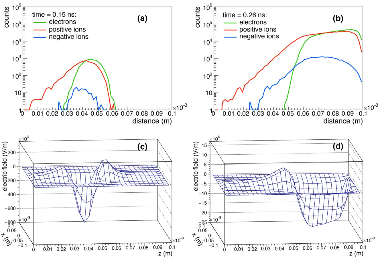
Electrons and ions are partially overlapped in space during the avalanche growth in the gas gap. Figures 5a and 5b show the number of electrons and ions along the gas gap at 0.15 ns and 0.26 ns, respectively. In this case, the number of electrons and ions as a function of the distance are evaluated in an avalanche originated from one single electron, which starts from the origin and at = 0 s. The MATOQ simulation is carried out in the gas mixture of 85% C2H2F4, 5% i-C4H10 and 10% SF6 at 296.15 K and 970 mbar with an applied electric field of 14 kV/mm. The overlap of positive and negative charges generates the space charge electric field along the gas gap. Values of the space charge electric field at 0.15 ns and 0.26 ns are shown in figures 5c and 5d, respectively. The MATOQ simulation results in figure 5 are consistent with the findings of Lippmann et al.’s model Lippmann and Riegler 2004. In particular, there are regions in the gas gap where the space charge electric field is decreased, while in other regions, it is increased. This effect becomes more evident during the evolution of the avalanche in both space and time.
A comparison between avalanche sizes at the anode simulated with MATOQ and those calculated with the Lippmann et al.’s model is presented in figure 6. The comparison is carried out in a 0.1-mm single-gap RPC, using a gas mixture of 85% C2H2F4, 5% i-C4H10 and 10% SF6 at 296.15 K and 970 mbar, for electric fields ranging from 6 kV/mm to 15 kV/mm. In addition, the average size of avalanches originating from a single electron at the cathode is calculated in the absence of space charge effects and shown in figure 6. The appearance of space charge effects during the avalanche development generally leads to a decrease in gas gain and reduced avalanche sizes Abbrescia et al. 2018. The agreement between the average sizes obtained from MATOQ simulations, with and without considering the space charge effects, is good for low electric field values. On the contrary, for electric field values higher than 12 kV/mm, the difference between the average avalanche size calculated with and without space charge effects becomes significant. Specifically, at 15 kV/mm, the average avalanche size without considering space charge effects is two orders of magnitude higher than that obtained by accounting for the space charge effects. Figure 6 also shows the average avalanche sizes computed using the Lippmann et al.’s model. The MATOQ simulation results with space charge effects exhibit good agreement with the calculations performed by Lippmann et al., except for electric field values below 11 kV/mm where there is a difference by a factor of approximately 2. There could be some reasons for the discrepancies between the results of the Lippmann et al.’s model and the MATOQ simulation. Firstly, the Lippmann et al.’s model generates avalanches using a pattern of initial electrons with an accurate estimation of their positions and energies, while all avalanches in MATOQ are generated by a single electron at the cathode with an initial energy of 5 eV. Secondly, there could be differences in the electron collision cross sections used in the model and in the simulation. Lippmann et al. used MAGBOLTZ 2.2 to evaluate electron transport coefficients and reaction rates, while MATOQ uses electron collision cross sections from different databases. In fact, electron collision cross sections of SF6 and i-C4H10 for the MATOQ simulation are the same as those implemented in MAGBOLTZ 10.6, whereas the cross sections for C2H2F4 are provided by Šašić et al. in their work published in 2013 Šašić et al. 2013.
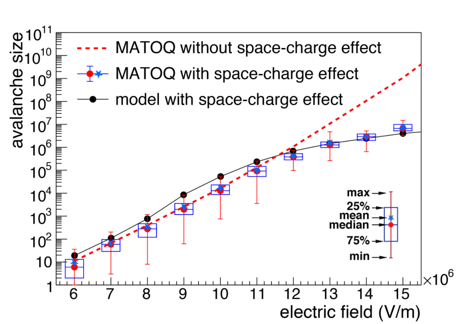
During testing the MATOQ code, a limitation has been found in the simulation of more than 5107 electrons. Indeed, several simulations of avalanches with this large number of electrons turned out to be incomplete probably because of a memory allocation limitation. The amount of simulation data to temporarily record might have saturated the available memory of the platform where the code was running. Nevertheless, this does not represent an important limitation if the gas gain is not too high, as in the case shown in figure 6. More details of the system where the MATOQ program is executed are provided in the appendix.
VIII Electron Transport Parameters in C3H2F4-based Gas Mixtures
The reduction of fluorinated greenhouse gas emissions in the European Union countries has been made mandatory by new regulations The European Parliament and the Council 2014 introduced since January 2015. The primary objective of the regulation is to gradually phase out hydrofluorocarbons (such as C2H2F4), currently available on the market, to limit their overall production. Even though research applications are exempt from current regulations, the phasing out of hydrofluorocarbons could gradually increase their price due to their limited future availability. A number of R&D studies Abbrescia et al. 2016a; Guida et al. 2016; Liberti et al. 2016; Bianchi et al. 2019 are ongoing to investigate the potential replacement of C2H2F4-based gas mixtures for RPCs with other more environmental-friendly gases. One alternative to C2H2F4 is C3H2F4, which appears to be a viable solution for RPCs. However, directly replacing C2H2F4 with C3H2F4 is not feasible due to the resulting high operating voltages of RPCs. A potential solution to address this issue is to replace C2H2F4 with a binary mixture of C2H2F4 and CO2 in varying proportions.
By using the MATOQ code, we can compare how the electron transport parameters vary in C2H2F4 and C3H2F4 as well as in gas mixtures of C3H2F4 and CO2 in different percentages. Figures 7a and 7b show the and in C2H2F4 and C3H2F4 as a function of the reduced electric field , respectively. In pure C2H2F4, values of and are higher than those in pure C3H2F4 between 10 Td and 300 Td. At a reduced electric field of 150 Td, the average electron energy is 5 eV in pure C2H2F4, while it is 3 eV in pure C3H2F4. These values are 7 eV and 4.5 eV at 300 Td. Similarly, the drift velocity in C3H2F4 at 150 Td is about three times lower than that in C2H2F4, with the reduction being about four times at 300 Td. When C3H2F4 is mixed with 50% or 60% of CO2, the values of and increase slightly as a function of , compared to those in pure C3H2F4, as shown in figures 7a and 7b. The increase of is 20% at both 150 Td and 300 Td. Similarly, in C3H2F4/CO2 mixtures is increased by approximately 20% at 150 Td compared to that in pure C3H2F4, whereas the increase is 25% at 300 Td.
Figure 8a shows the positive values of the effective ionization Townsend coefficient as a function of in pure C2H2F4, pure C3H2F4, and C3H2F4-based gas mixtures with 50% or 60% CO2. These values are reported to identify the reduced electric field values at which electron avalanches can occur in RPCs. For pure C2H2F4, the effective ionization Townsend coefficient is higher than 0, indicating that ionization events occur more frequently than attachment events, at a reduced electric field of 50 Td. On the contrary, the electron avalanche growth can occur at 290 Td in pure C3H2F4. When C3H2F4 is diluted with CO2, the growth of electron avalanches occurs at lower values of the electric field, as reported by experimental studies Bianchi et al. 2019; Proto et al. 2022; Abbrescia et al. 2016b; Rigoletti et al. 2020; Bianchi et al. 2021. This observation is also supported by MATOQ simulations. Indeed, in a gas mixture with equal proportions of C3H2F4 and CO2, begins to exceed 0 at 190 Td. If the CO2 percentage is increased from 50% to 60%, ionization events are more frequent than attachment events starting from 170 Td. Figure 8b shows the ionization Townsend coefficient and the attachment Townsend coefficient as a function of in C3H2F4-based gas mixture with the addition of 50% of CO2 or 60% of CO2. As shown in figure 8b, values of increase progressively with , whereas values of tend to reach a plateau after the initial growth.
The replacement of C2H2F4 with C3H2F4 requires dedicated studies also in narrow-gap RPCs, where the effect of space charge electric field may play a crucial role. Figure 9 presents the average avalanche size at the anode in a 0.1-mm single-gap RPC. The simulation is carried out for a range of applied electric fields from 6 kV/mm to 15 kV/mm, including the space charge effects in the gas gap and using the gas mixture consisting of 85% C2H2F4, 5% i-C4H10 and 10% SF6 at 296.15 K and 970 mbar. Additionally, the simulations are performed by replacing C2H2F4 with an equal amount of C3H2F4. In the C3H2F4-based gas mixture, the average avalanche size follows an exponential trend until approximately 10 kV/mm. At low electric field values, the average avalanche size is reduced by a factor of 20 to 30 when C2H2F4 is replaced with C3H2F4. On the contrary, the average avalanche size in the C3H2F4-based gas mixture is approximately 58 times smaller than that in the C2H2F4-based gas mixture at high electric field values.
IX Conclusions
The MATOQ program has been developed to study environmental-friendly gas mixtures for RPCs. This program enables the simulation of electron transport coefficients and reaction rates in gases under the influence of an electric field. Mean energy and drift velocity of electrons as well as ionization and attachment coefficients are evaluated both in temporal and in spatial growth configurations. Unlike the already existing programs, the MATOQ code also allows the evaluation of space charge effects between electrons and ions during the development of the electron avalanche. MATOQ is written in C++, which makes it a multi-platform software, and supports the multi-thread execution, which speeds the computation time. The data format of electron collision cross sections adopted in the LXCat database, which is widely used and regularly upgraded, is compatible with MATOQ.
The temporal and spatial growth configurations of electron avalanches under the influence of uniform electric fields have been validated by comparing the MATOQ results with those obtained by MAGBOLTZ. The electron transport coefficients and reaction rates, namely , , , , and , show good agreement with experimental data in pure Ar, N2, CO2 and in the binary mixture of 50% Ar and 50% N2. Moreover, the simulation of electron avalanches influenced by both uniform and space charge electric fields is validated by comparing the avalanche sizes obtained from MATOQ to those calculated using Lippmann et al.’s model.
According to several experimental R&D studies, one potential alternative to C2H2F4 in RPCs is C3H2F4, which is considered to be more environmentally friendly. Using MATOQ, we calculated the changes in electron transport coefficients and reaction rates in pure C2H2F4 and C3H2F4, as well as in gas mixtures of C3H2F4 and CO2 in various proportions. The dilution of C3H2F4 with CO2 is considered a viable solution for operating RPCs within the voltage range currently used. This solution may also be applicable to narrow-gap RPCs. Indeed, the simulations conducted using MATOQ suggest that the average avalanche size is reduced approximately by one order of magnitude when C2H2F4 is only replaced with C3H2F4 in a 0.1-mm single-gap RPC.
Appendix
All sets of electron collision cross sections used in this work as input for MATOQ are summarized in table 1:
| Gas | Source |
|---|---|
| Ar | LXCat: Biagi’s database MAGBOLTZ v8.97 lxc |
| N2 | LXCat: Biagi’s database MAGBOLTZ v8.97 lxc |
| CO2 | LXCat: Biagi’s database MAGBOLTZ v11.6 lxc |
| C2H2F4 | Šašić et al. Šašić et al. 2013 |
| C3H2F4 | Bianchi et al. Bianchi et al. 2021 |
| i-C4H10 | MAGBOLTZ v10.6 Biagi 1999 |
| SF6 | LXCat: Biagi’s database MAGBOLTZ v10.6 lxc |
Comparisons between MATOQ and MAGBOLTZ calculations in figures 2 and 3 are carried out by using the version 8.97 of MAGBOLTZ in the case of Ar and N2, whereas the version 11.6 of MAGBOLTZ is used for the result simulations in pure CO2, according to table 1.
The MATOQ program is interfaced with the software ROOT, freely provided by the European Organization for Nuclear Research (CERN), to plot the results during the simulation Antcheva et al. 2011.
All simulations of this work have been performed in the virtual machines of the Linux Public Login User Service (LXPLUX7) provided by CERN. These machines are organized in a cluster of PCs running CERN CentOS Linux in 64-bit mode. More details can be found in the LXPLUS7 documentation.
DATA AVAILABILITY
The data that support the findings of this study are available from the corresponding author upon reasonable request.
References
- Santonico and Cardarelli (1981) R. Santonico and R. Cardarelli, Development of Resistive Plate Counters, Nuclear Instruments and Methods in physics research 187, 377 (1981).
- Bruno (2004) G. Bruno, Resistive Plate Chambers in running and future experiments, The European Physical Journal C-Particles and Fields 33, s1032 (2004).
- Abbrescia et al. (2012) M. Abbrescia, S. Aiola, R. Antolini, C. Avanzini, R. B. Ferroli, G. Bencivenni, E. Bossini, E. Bressan, A. Chiavassa, C. Cicalo, et al., The EEE project: cosmic rays, multigap Resistive Plate Chambers and high school students, Journal of Instrumentation 7 (11), P11011.
- Zeballos et al. (1996a) E. C. Zeballos, I. Crotty, D. Hatzifotiadou, J. L. Valverde, S. Neupane, M. Williams, and A. Zichichi, A new type of Resistive Plate Chamber: The Multigap RPC, Nuclear Instruments and Methods in Physics Research Section A: Accelerators, Spectrometers, Detectors and Associated Equipment 374, 132 (1996a).
- Amaldi et al. (2015) U. Amaldi, G. Borghi, M. Bucciantonio, R. Kieffer, J. Samarati, F. Sauli, and D. Watts, Development of TOF-PET detectors based on the multi-gap Resistive Plate Chambers, Nuclear Instruments and Methods in Physics Research Section A: Accelerators, Spectrometers, Detectors and Associated Equipment 778, 85 (2015).
- Crespo et al. (2013) P. Crespo, A. Blanco, M. Couceiro, N. C. Ferreira, L. Lopes, P. Martins, R. Ferreira Marques, and P. Fonte, Resistive Plate Chambers in positron emission tomography, The European Physical Journal Plus 128, 1 (2013).
- Intergovernmental Panel on Climate Change (2014) (IPCC) Intergovernmental Panel on Climate Change (IPCC), Fifth assessment report (2014).
- Abbrescia et al. (2016a) M. Abbrescia, L. Benussi, D. Piccolo, S. Bianco, M. Ferrini, S. Muhammad, L. Passamonti, D. Pierluigi, F. Primavera, A. Russo, et al., Eco-friendly gas mixtures for Resistive Plate Chambers based on tetrafluoropropene and helium, Journal of Instrumentation 11 (08), P08019.
- Guida et al. (2016) R. Guida, M. Capeans, and B. Mandelli, Characterization of RPC operation with new environmental friendly mixtures for LHC application and beyond, Journal of Instrumentation 11 (07), C07016.
- Liberti et al. (2016) B. Liberti, G. Aielli, P. Camarri, R. Cardarelli, A. Di Ciaccio, L. Di Stante, E. Pastori, and R. Santonico, Further gas mixtures with low environment impact, Journal of Instrumentation 11 (09), C09012.
- Bianchi et al. (2019) A. Bianchi, S. Delsanto, P. Dupieux, A. Ferretti, M. Gagliardi, B. Joly, S. Manen, M. Marchisone, L. Micheletti, A. Rosano, et al., Characterization of tetrafluoropropene-based gas mixtures for the Resistive Plate Chambers of the ALICE muon spectrometer, Journal of Instrumentation 14 (11), P11014.
- Proto et al. (2022) G. Proto, B. Liberti, R. Santonico, G. Aielli, P. Camarri, R. Cardarelli, A. Di Ciaccio, L. Di Stante, A. Paoloni, E. Pastori, et al., On a new environment-friendly gas mixture for Resistive Plate Chambers, Journal of Instrumentation 17 (05), P05005.
- Abbrescia et al. (2016b) M. Abbrescia, P. Van Auwegem, L. Benussi, S. Bianco, S. Cauwenbergh, M. Ferrini, S. Muhammad, L. Passamonti, D. Pierluigi, D. Piccolo, et al., Preliminary results of Resistive Plate Chambers operated with eco-friendly gas mixtures for application in the CMS experiment, Journal of Instrumentation 11 (09), C09018.
- Rigoletti et al. (2020) G. Rigoletti, G. Aielli, G. Alberghi, L. Benussi, A. Bianchi, S. Bianco, L. Di Stante, D. Boscherini, A. Bruni, P. Camarri, et al., Studies of RPC detector operation with eco-friendly gas mixtures under irradiation at the CERN Gamma Irradiation Facility, POS Proceedings of Science 364, 164 (2020).
- Chachereau et al. (2016) A. Chachereau, M. Rabie, and C. M. Franck, Electron swarm parameters of the hydrofluoroolefine hfo1234ze, Plasma Sources Science and Technology 25, 045005 (2016).
- Bianchi et al. (2020) A. Bianchi, S. Delsanto, P. Dupieux, A. Ferretti, M. Gagliardi, B. Joly, S. Manen, M. Marchisone, L. Micheletti, A. Rosano, et al., Studies on tetrafluoropropene-based gas mixtures with low environmental impact for Resistive Plate Chambers, Journal of Instrumentation 15 (04), C04039.
- Biagi (1999) S. Biagi, Monte Carlo simulation of electron drift and diffusion in counting gases under the influence of electric and magnetic fields, Nuclear Instruments and Methods in Physics Research Section A 421, 234 (1999).
- Bianchi et al. (2021) A. Bianchi, A. Ferretti, M. Gagliardi, and E. Vercellin, Electron collision cross sections in tetrafluoropropene HFO1234ze, arXiv preprint arXiv:2103.08643 (2021).
- Rabie and Franck (2016) M. Rabie and C. M. Franck, METHES: A Monte Carlo collision code for the simulation of electron transport in low temperature plasmas, Computer Physics Communications 203, 268 (2016).
- Pancheshnyi et al. (2012) S. Pancheshnyi, S. Biagi, M. Bordage, G. Hagelaar, W. Morgan, A. Phelps, and L. Pitchford, The LXCat project: Electron scattering cross sections and swarm parameters for low temperature plasma modeling, Chemical Physics 398, 148 (2012).
- Dagum and Menon (1998) L. Dagum and R. Menon, OpenMP: an industry standard API for shared-memory programming, IEEE computational science and engineering 5, 46 (1998).
- Antcheva et al. (2011) I. Antcheva, M. Ballintijn, B. Bellenot, M. Biskup, R. Brun, N. Buncic, P. Canal, D. Casadei, O. Couet, V. Fine, et al., ROOT: A C++ framework for petabyte data storage, statistical analysis and visualization, Computer Physics Communications 182, 1384 (2011).
- Abbrescia et al. (2018) M. Abbrescia, P. Fonte, and V. Peskov, Resistive Gaseous Detectors: designs, performance, and perspectives (Wiley-VCH, Weinheim, 2018).
- Zeballos et al. (1996b) E. C. Zeballos, I. Crotty, D. Hatzifotiadou, J. L. Valverde, S. Neupane, M. Williams, and A. Zichichi, A new type of Resistive Plate Chamber: the multigap RPC, Nuclear Instruments and Methods in Physics Research Section A 374, 132 (1996b).
- Lippmann and Riegler (2004) C. Lippmann and W. Riegler, Space charge effects in Resistive Plate Chambers, Nuclear Instruments and Methods in Physics Research Section A: Accelerators, Spectrometers, Detectors and Associated Equipment 517, 54 (2004).
- Skullerud (1968) H. Skullerud, The stochastic computer simulation of ion motion in a gas subjected to a constant electric field, Journal of Physics D: Applied Physics 1, 1567 (1968).
- Koura (1986) K. Koura, Null-collision technique in the direct-simulation Monte Carlo method, The Physics of fluids 29, 3509 (1986).
- Landau and Lifshitz (2013) L. D. Landau and E. M. Lifshitz, Mechanics and electrodynamics (Elsevier, 2013).
- Šašić et al. (2013) O. Šašić, S. Dupljanin, J. de Urquijo, and Z. L. Petrović, Scattering cross sections for electrons in C2H2F4 and its mixtures with Ar from measured transport coefficients, Journal of Physics D: Applied Physics 46, 325201 (2013).
- The European Parliament and the Council (2014) The European Parliament and the Council, Regulation (EU) no 517/2014 on fluorinated greenhouse gases, Official Journal of the European Union L 150, 195 (2014).
- (31) Biagi’s database, www.lxcat.net, retrieved in January, 2020.
*