The Adaptive $\tau$ -Lasso: Robustness and Oracle Properties

Emadaldin Mozafari-Majd Visa Koivunen

Abstract

This paper introduces a new regularized version of the robust $\tau$ -regression estimator for analyzing high-dimensional datasets subject to gross contamination in the response variables and covariates (explanatory variables). The resulting estimator, termed adaptive $\tau$ -Lasso, is robust to outliers and high-leverage points. It also incorporates an adaptive $\ell_{1}$ -norm penalty term, which enables the selection of relevant variables and reduces the bias associated with large true regression coefficients. More specifically, this adaptive $\ell_{1}$ -norm penalty term assigns a weight to each regression coefficient. For a fixed number of predictors $p$ , we show that the adaptive $\tau$ -Lasso has the oracle property, ensuring both variable-selection consistency and asymptotic normality under fairly mild conditions. Asymptotic normality applies only to the entries of the regression vector corresponding to the true support, assuming knowledge of the true regression vector support. We characterize its robustness by establishing the finite-sample breakdown point and the influence function. We carry out extensive simulations and observe that the class of $\tau$ -Lasso estimators exhibits robustness and reliable performance in both contaminated and uncontaminated data settings. We also validate our theoretical findings on robustness properties through simulations. In the face of outliers and high-leverage points, the adaptive $\tau$ -Lasso and $\tau$ -Lasso estimators achieve the best performance or match the best performances of competing regularized estimators, with minimal or no loss in terms of prediction and variable selection accuracy for almost all scenarios considered in this study. Therefore, the adaptive $\tau$ -Lasso and $\tau$ -Lasso estimators provide attractive tools for a variety of sparse linear regression problems, particularly in high-dimensional settings and when the data is contaminated by outliers and high-leverage points. However, it is worth noting that no particular estimator uniformly dominates others in all considered scenarios.

Index Terms:

robust estimator, sparsity, high-dimensional data, linear regression, regularized estimator, variable selection, oracle property, asymptotic normality, consistency, influence function, root-

n

consistency, breakdown point.

I Introduction

The last two decades have witnessed a phenomenal surge in the collection and acquisition of large volumes of data with an increasing number of features or predictors [1, 2, 3]. Formidable challenges arise with high-dimensional models where the number of features $(p)$ exceeds the number of observations $(n)$ , causing problems with uniqueness and identifiability. Such high-dimensional data often encompass a low-dimensional representation due to sparsity or a low-rank structure. Indeed, if there is no underlying structure, one may be unable to recover useful information from data about parameters of interest with a low sample size $n$ . Thus, regularization of the ill-defined estimation problem may be necessary to find a unique solution and capture a low-dimensional representation of the high-dimensional data. In the sparse linear regression settings, it is common to regularize the empirical loss by the $\ell_{1}$ -norm of the parameter vector to promote sparsity. Regularizing the squared-error loss by $\ell_{1}$ -norm gives rise to the celebrated Lasso estimator that combines variable selection with parameter estimation. While the $\ell_{1}$ -norm penalty reduces the variance of the estimated values, it may overshrink the coefficient estimates [4] when the true coefficients are large and produce very biased estimates. Adaptive Lasso [5] substitutes the $\ell_{1}$ -norm penalty with an adaptive $\ell_{1}$ -norm penalty where small weights are given to parameters associated with large true coefficients. This adjustment reduces the penalty imposed on these parameters, leading to estimates with lower bias. The modified Lasso estimator (adaptive Lasso), as described above, satisfies oracle properties, i.e., (i) the support of the estimated coefficient vector agrees with the support of the true coefficient vector in the asymptotic sense (variable selection consistency); (ii) asymptotic normality holds for the entries of the regression vector corresponding to the true support by knowing the correct support a priori.

An important issue in dealing with high-dimensional models is that the probability of observing outliers or high-leverage points may increase as the sample size and dimensionality grow together. Moreover, one must take special care when the distribution of covariates or additive noise is heavy-tailed. The regularized least-squares estimators exhibit poor performance in the presence of contamination or heavy-tailed noise as the squared-error loss is highly sensitive to outliers and high-leverage points, i.e., it is not statistically robust. In order to address this issue, one can replace the squared-error loss with a robust counterpart that grows more slowly for larger residuals. This approach gives smaller weights to data points with large residuals. Examples include absolute-error loss, Huberized loss, and $\ell_{q}$ -based losses with $1<q<2$ . These loss functions are robust in the face of outliers and other contaminations. There is a large body of methods using regularized M-estimators with a convex empirical loss [6, 7, 8, 9, 10, 11, 12, 13, 14, 15, 16, 17, 18]. Despite strong theoretical guarantees, these estimators may fail to limit the influence of high-leverage points in the covariates and hence may lead to a significant decrease in performance. Several procedures have been proposed to mitigate the influence of high-leverage points, particularly in [13, 18]. These procedures either down-weight the observations with outlying predictor values or truncate all predictor values via univariate winsorization, even when only one predictor in the corresponding observation is an outlier. Neither of these characteristics is desirable in high-dimensional models. Additionally, there is a collection of regularized robust linear estimators introduced in [6]. Two of these replace the data-discrepancy term (empirical cost term) with non-convex losses, such as $\ell_{q}$ -based norms (with $0<q<1$ ) and Lorentzian-based norms of residuals, that can be tuned to grow more slowly than the absolute-error loss for larger residuals. However, they still struggle to handle high-leverage points, and in particular, $\ell_{q}$ -norms become extremely non-smooth as $q$ approaches zero.

Motivated by this deficiency of convex empirical losses, several regularized linear regression estimators robust to high-leverage points have been developed. Regularized robust linear regression estimators, known as MM-Lasso and adaptive MM-Lasso, were proposed in [19]. These estimators substitute the squared-error loss of Lasso with a non-convex loss that features a redescending score function [20]. In addition, the authors provide a solid foundation for analyzing the behavior of these estimators by deriving the robustness properties and the asymptotic theory for consistency. Other important related works include adaptive penalized elastic net S-estimator (adaptive PENSE) [21] and penalized elastic net S-estimator (PENSE) [22], both of which demonstrate favorable robustness properties and have established the asymptotic theory for consistency.

This paper introduces the adaptive $\tau$ -Lasso estimator, a low-dimensional $\tau$ -estimator regularized by an adaptive $\ell_{1}$ -norm penalty similar to adaptive lasso [5]. The present study extends the work of Martinez-Camara et al. [23, 24], who initially proposed the $\tau$ -Lasso estimator and derived its influence function. A major drawback of $\tau$ -Lasso is that variable selection consistency holds under restrictive mutual incoherence assumptions on the design matrix $\mathbf{X}$ present in the $\ell_{1}$ -based methods [25]. With the motivation of addressing this, we modify the $\tau$ -Lasso objective function by replacing the $\ell_{1}$ -norm penalty with an adaptive $\ell_{1}$ -norm penalty. This modification dispenses the need for mutual incoherence conditions required by the $\tau$ -Lasso estimator, thereby yielding a variable selection consistent procedure under fairly mild conditions on the loss function, the decay rate of the regularization parameter and the data distribution. Herein, we focus on regularized versions of $\tau$ -estimators [26, 27] and establish robustness and asymptotic properties when data follows a sparse linear regression model. We emphasize that the asymptotic theory established in this paper is constrained to the classical fixed $p$ and diverging $n$ and holds even for very heavy-tailed errors such as Cauchy-distributed noise/errors.

We now summarize the main new contributions of the paper as follows:

•

The asymptotic theory for consistency of the $\tau$ -Lasso estimator, including strong and root- $n$ consistency, is derived.
•

The adaptive $\tau$ -Lasso estimator is introduced, and its oracle properties are established under relatively mild conditions. To do so, we first show the estimator’s asymptotic normality for the entries of the regression vector corresponding to the true support when the correct support is known a priori. We then prove variable selection consistency without imposing any conditions on the moments of the error distribution. This is an advantage over its predecessor $\tau$ -Lasso, which does not achieve variable consistency unless under stringent conditions on the design matrix.
•

The global robustness properties of the adaptive $\tau$ -Lasso estimator, as measured by its finite-sample breakdown, are characterized. Moreover, we provide a lower and upper bound on the finite-sample breakdown point. Subsequently, the estimator’s high breakdown point is validated via computer simulations.
•

We derive the influence function of the adaptive $\tau$ -Lasso estimator. We also verify from our simulation results that the resulting influence function agrees with its finite-sample version, standardized sensitivity curve, for one-dimensional toy data.
•

Extensive simulation studies are conducted where the finite-sample performance of $\tau$ -Lasso and adaptive $\tau$ -Lasso is compared to that of other competing state-of-the-art regularized robust linear regression estimators on synthetic and real data.
•

The influence of pilot estimates on the adaptive $\tau$ -Lasso’s performance has been investigated. Additionally, we present an example encountered in practical settings, where good leverage points are found on truly irrelevant predictors, and showcase adaptive $\tau$ -Lasso significantly outperforms $\tau$ -Lasso in variable selection (provided in Supplemental Material). Moreover, the phenomenon of overshrinkage in $\tau$ -Lasso is studied and confirmed through simulations that adaptive $\tau$ -Lasso effectively remedies this issue.

I-A Related work

There are close connections between our adaptive $\tau$ -Lasso estimator and several other high-dimensional regularized robust linear estimators: the adaptive MM-Lasso estimator [19], the adaptive penalized elastic-net S-estimator (adaptive PENSE) [21], and the $\tau$ -Lasso estimator [24], [23], all of which deal with high-leverage points in the predictors. We highlight the similarities and differences between our adaptive $\tau$ -Lasso estimator and these estimators.

•

Adaptive $\tau$ -Lasso, $\tau$ -Lasso and adaptive MM-Lasso estimators can simultaneously achieve a high breakdown point and high normal efficiency.
•

Moreover, the adaptive MM-Lasso and adaptive PENSE estimators, like the adaptive $\tau$ -Lasso, enjoy oracle properties for a fixed number of covariates $p$ under fairly mild conditions. This is a by-product of substituting the $\ell_{1}$ -norm penalty with an adaptive $\ell_{1}$ -norm penalty.
•

While our proposed estimator enjoys oracle properties even for heavy-tailed errors under fairly mild conditions, the $\tau$ -Lasso estimator suffers from the overshrinkage problem associated with the $\ell_{1}$ -norm penalty. In fact, $\tau$ -Lasso achieves variable selection consistency under restrictive mutual incoherence conditions, which is not trivial.
•

The adaptive MM-Lasso requires a preliminary robust estimate of the scale of the additive errors. High efficiency under normal errors can be attained if bias in M-scale estimation remains small, which is often challenging in high-dimensional settings.
•

The adaptive PENSE circumvents the need for a preliminary scale estimate of additive errors and achieves high-breakdown points, but it can not be tuned for high normal efficiency.
•

In contrast, our adaptive $\tau$ -Lasso achieves both high breakdown and high normal efficiency without requiring a preliminary estimate of the scale of additive errors, as it is naturally associated with an estimate of the error scale, known as $\tau$ -scale.

However, it is important to acknowledge that in the high-dimensional regime, if bias associated with M-scale of the residuals is large, the high normal efficiency of the adaptive $\tau$ -Lasso may be compromised, particularly under contamination in finite-sample settings.

I-B Organization

The remainder of this paper is organized as follows. Section II details the basic notation used throughout the paper. Section III describes the data model used in this article in detail. Section IV introduces the background material on the adaptive $\tau$ -Lasso estimator. We then provide the main results in Section V, including theorems and propositions on the asymptotic properties of the $\tau$ -Lasso and adaptive $\tau$ -Lasso estimators. Section VI is devoted to characterizing the robustness properties such as finite-sample breakdown point and influence function for the adaptive $\tau$ -Lasso estimator. In Section VII, we illustrate the simulation results for the $\tau$ -Lasso and the adaptive $\tau$ -Lasso estimators and compare the results with other competing regularized robust estimators for several scenarios. We then conclude the paper in Section VIII. We defer full proofs and technical derivations of the theoretical results outlined in this paper to the Supplemental Material, given their lengthy and tedious nature.

II Notation

Given the true regression parameter vector (coefficient vector) $\boldsymbol{\beta}_{0}\in\mathbb{R}^{p}$ , we denote by $\mathcal{A}\coloneqq\{j\in\{1,\cdots,p\}|\beta_{0,j}\neq 0\}$ the true active set corresponding to the set of predictors associated with true non-zero coefficients and $\mathcal{A}^{c}\coloneqq\{j\in\{1,\cdots,p\}|\beta_{0,j}=0\}$ the true inactive set corresponding to the set of predictors associated with true zero coefficients. To simplify the matters with proofs of theorems, without loss of generality, we assume that the first $k_{0}>0$ elements of $\boldsymbol{\beta}_{0}$ are non-zero and thus the true active set $\mathcal{A}\coloneqq\{1,2,\cdots,k_{0}\}$ . We write $\mathbf{X}_{\mathcal{A}}$ to denote the regression matrix whose columns are those predictors in $\mathcal{A}$ . For a vector $\boldsymbol{\beta}\in\mathbb{R}^{p}$ , we denote by $\boldsymbol{\beta}_{\mathcal{A}}$ the first $k_{0}$ coefficients of $\boldsymbol{\beta}$ and $\boldsymbol{\beta}_{\mathcal{A}^{c}}$ the remaining $p-k_{0}$ coefficients of $\boldsymbol{\beta}$ . Furthermore, we note the $\ell_{1}$ -norm as

\|\boldsymbol{\beta}\|_{\ell_{1}}=\sum_{j=1}^{p}|\beta_{j}|.

(1)

To avoid confusion, we provide the reader with a list of notations that will be consistently used within the body of the proofs.

List of Notations

$\hat{\boldsymbol{\beta}}_{\text{PT}}$

$\tau$ -Lasso estimator.
$\hat{\boldsymbol{\beta}}_{\text{AT}}$

Adaptive $\tau$ -Lasso estimator.
$\hat{\boldsymbol{\beta}}_{\text{T}}$

$\tau$ -estimator.
$\tilde{\boldsymbol{\beta}}$

Pilot estimate of $\boldsymbol{\beta}_{0}$ employed to compute the adaptive weights $w_{j}$ .
$\partial_{\boldsymbol{\beta}}(f)$

Generalized gradient of $f$ with respect to $\boldsymbol{\beta}$ .
$\underline{\mathcal{L}}_{n}(\boldsymbol{\beta})$

Objective function of the $\tau$ -Lasso estimator evaluated at $\boldsymbol{\beta}$ .
$\mathcal{L}_{n}(\boldsymbol{\beta})$

Objective function of the adaptive $\tau$ -Lasso estimator evaluated at $\boldsymbol{\beta}$ .
$\mathbf{x}$

$p$ -dimensional random vector of predictors.
$y$

Random response variable.
$u$

Random measurement noise variable.
$r(\boldsymbol{\beta}_{0})$

True error, $r(\boldsymbol{\beta}_{0})\coloneqq y-\mathbf{x}^{T}\boldsymbol{\beta}_{0}=u$ (r.v.).
$\tau_{n}(\mathbf{r}(\boldsymbol{\beta}))$

$\tau$ -scale estimate of the residual vector $\mathbf{r}(\boldsymbol{\beta})$ .
$\tau(\boldsymbol{\beta}_{0})$

Population $\tau$ -scale of the true error, $\tau(r(\boldsymbol{\beta}_{0}))$ , we allow a small violation of notation for simplicity.
$s_{n}(\mathbf{r}(\boldsymbol{\beta}))$

M-scale estimate of the residual vector $\mathbf{r}(\boldsymbol{\beta})$ .
$s(\boldsymbol{\beta}_{0})$

Population M-scale of the true error, $s(r(\boldsymbol{\beta}_{0}))$ , we allow a small violation of notation for simplicity.
$\delta$

Tuning parameter set to a desired value for controlling the asymptotic breakdown point of the estimator.
$\delta^{*}$

Constant defining the desired asymptotic breakdown point of the estimator.
$\zeta^{*}$

Constant defining the desired normal efficiency.
$c_{0}$

Tuning parameter of $\rho_{0}(\cdot)$ adjusted to achieve the desired asymptotic breakdown point.
$c_{1}$

Tuning parameter of $\rho_{1}(\cdot)$ adjusted to achieve the desired normal efficiency for a known $c_{0}$ .
$\underline{\lambda}_{n}$

Regularization parameter of the $\tau$ -Lasso estimator, assumed to vary with sample size $n$ as required for the asymptotic analysis.
$\lambda_{n}$

Regularization parameter of the adaptive $\tau$ -Lasso estimator, assumed to vary with sample size $n$ as required for the asymptotic analysis.
$\mathbb{E}_{F}(\cdot)$

Expected value with respect to distribution $F$ .
$\theta_{n}=o_{P}(a_{n})$

Implies that the sequence $\lVert\theta_{n}\rVert_{\ell_{2}}/\lvert a_{n}\rvert$ converges to zero in probability [28].
$\theta_{n}=O_{P}(a_{n})$

Implies that the sequence $\lVert\theta_{n}\rVert_{\ell_{2}}/\lvert a_{n}\rvert$ is bounded in probability (or uniformly tight) [28].
$\mathbb{P}(\cdot)$

Probability of an event.

III Data Model

Throughout this article, we assume data follows a sparse linear regression model

\mathbf{y}=\mathbf{X}\boldsymbol{\beta}_{0}+\mathbf{u},

(2)

where $\mathbf{y}=[y_{1},\cdots,y_{n}]^{T}\in\mathbb{R}^{n}$ denotes the response vector, $\mathbf{X}=[\mathbf{x}_{[1]},\cdots,\mathbf{x}_{[n]}]^{T}\in\mathbb{R}^{n\times p}$ is the regression matrix and data pairs $\{(y_{i},\mathbf{x}_{[i]})\}_{i=1}^{n}$ are $n$ i.i.d. realizations of random variable $(y,\mathbf{x})\in\mathbb{R}\times\mathbb{R}^{p}$ . $\mathbf{u}=[u_{1},\cdots,u_{n}]^{T}\in\mathbb{R}^{n}$ is the measurement noise vector where $\{u_{i}\in\mathbb{R}\}_{i=1}^{n}$ are $n$ i.i.d. realizations of random variable $u\in\mathbb{R}$ . The goal is to estimate the unknown sparse parameter vector $\boldsymbol{\beta}_{0}\in\mathbb{R}^{p}$ based on a sample of $n$ observations $\big(\mathbf{y},\mathbf{X}\big)$ . We assume sparsity such that $k_{0}<p$ coefficients of $\boldsymbol{\beta}_{0}$ are non-zero, and their corresponding indices and $k_{0}$ are not known in advance.

Suppose the measurement errors $u_{i}$ follow some distribution $F$ and are independent of the explanatory variables $\mathbf{x}_{[i]}$ with distribution $G$ . Then, the joint distribution $H$ of $(y_{i},\mathbf{x}_{[i]})$ satisfy

H(y,\mathbf{x})=G(\mathbf{x})F(y-\mathbf{x}^{T}\boldsymbol{\beta}_{0}).

(3)

Here, it is crucial to distinguish between $y$ , $\mathbf{x}$ , and $u$ , which are random variables and their corresponding realizations $y_{i}$ , $\mathbf{x}_{[i]}$ , and $u_{i}$ , which are deterministic. This distinction is of paramount importance as it significantly impacts the subsequent statistical analysis discussed in this article.

IV The Adaptive $\tau$ -Lasso

IV-A Definition

The $\tau$ -Lasso estimator [23, 24] is a regularized robust estimator whose objective function comprises a regularization term to deal with high-dimensional models and a robust empirical loss to deal with outliers and high-leverage points. While $\ell_{1}$ -norm regularization of the $\tau$ -Lasso promotes sparsity by setting some coefficients to zero, which is a desired property, it also severely shrinks the estimated coefficients associated with larger true coefficients. In order to remedy the overshrinkage of the $\tau$ -Lasso estimates for these coefficients, one can assign properly chosen weights to different regression coefficients similarly to the adaptive Lasso [5]. We now introduce the adaptive $\tau$ -Lasso as

\hat{\boldsymbol{\beta}}_{\text{AT}}=\argmin_{\boldsymbol{\beta}\in\mathbb{R}^{p}}\mathcal{L}_{n}(\boldsymbol{\beta})=\argmin_{\boldsymbol{\beta}\in\mathbb{R}^{p}}\biggl\{\tau_{n}^{2}(\mathbf{r}(\boldsymbol{\beta}))+\lambda_{n}\sum_{j=1}^{p}w_{j}|\beta_{j}|\biggl\}

(4)

where $\lambda_{n}$ is a nonnegative regularization parameter controlling the amount of shrinkage induced by the adaptive penalty term, and adaptive weights are given by $w_{j}=1/|\tilde{\beta}_{j}|^{\gamma}$ . $\tilde{\boldsymbol{\beta}}$ denotes a pilot estimate of $\boldsymbol{\beta}_{0}$ . The choice of $\gamma>0$ influences the variable selection consistency and asymptotic normality of the estimator and should be carefully selected to attain the desired results. We will, later on, show that if the pilot estimate $\tilde{\boldsymbol{\beta}}$ is a strongly consistent estimate of $\boldsymbol{\beta}_{0}$ , the adaptive $\tau$ -Lasso estimator enjoys the root- $n$ consistency and oracle properties with a proper selection of $\lambda_{n}$ under fairly mild conditions. Note that $\lambda_{n}$ varies with $n$ in the asymptotic analysis. Let $\mathbf{r}(\boldsymbol{\beta})=\mathbf{y}-\mathbf{X}\boldsymbol{\beta}$ be the vector of residuals, and let $\rho_{0}(\cdot)$ and $\rho_{1}(\cdot)$ represent bounded- $\rho$ -functions, as described in Assumption $1$ in the following lines. Then $\tau_{n}(\mathbf{r}(\boldsymbol{\beta}))$ is an efficient $\tau$ -scale [26, 27] defined as follows:

\tau_{n}^{2}(\mathbf{r}(\boldsymbol{\beta}))=s_{n}^{2}(\mathbf{r}(\boldsymbol{\beta}))\frac{1}{n}\sum_{i=1}^{n}\rho_{1}\bigg(\frac{r_{i}(\boldsymbol{\beta})}{s_{n}(\mathbf{r}(\boldsymbol{\beta}))}\bigg)

(5)

with $r_{i}(\boldsymbol{\beta})$ ’s denoting the residuals $\{y_{i}-\mathbf{x}_{[i]}^{T}\boldsymbol{\beta}\}$ and $s_{n}(\mathbf{r}(\boldsymbol{\beta}))$ is an M-scale estimate of residuals $\mathbf{r}(\boldsymbol{\beta})$ defined as the solution to

\frac{1}{n}\sum_{i=1}^{n}\rho_{0}\bigg(\frac{r_{i}(\boldsymbol{\beta})}{s_{n}(\mathbf{r}(\boldsymbol{\beta}))}\bigg)=\delta,

(6)

where $\delta$ is tuned to control the asymptotic breakdown point of the estimator; to simplify notation, we will write $\tau_{n}=\tau_{n}(\mathbf{r}(\boldsymbol{\beta}))$ and $s_{n}=s_{n}(\mathbf{r}(\boldsymbol{\beta}))$ . To ensure the robustness of our estimates, we need to impose several assumptions on our bounded $\rho$ -functions, $\rho_{0}(\cdot)$ and $\rho_{1}(\cdot)$ , as follows:

Assumption 1: the $\rho$ -functions in this work satisfy the following conditions [20, 21]

1.

$\rho(\cdot)$ is real, even, continuous and $\rho(0)=0$ .
2.

$\rho(t)$ is bounded where $\rho(t)=1$ for $|t|\geq c$ with $0<c<\infty$ , and is strictly increasing in $|t|$ elsewhere.
3.

$\rho(t)$ is continuously differentiable with both $t\rho^{{}^{\prime}}(t)$ and $\rho^{{}^{\prime}}(t)$ being bounded.

We note $\rho_{i}(t)=\rho(t\>;c_{i})$ where $i\in 0,1$ . Detailed instructions on tuning the constants $c_{0}$ and $c_{1}$ to achieve high breakdown point and high normal efficiency are given in Section S.I of the Supplemental Material.

Assumption 2:

2\rho_{1}(t)-\psi_{1}(t)t\geq 0,

(7)

where $\psi_{1}(t)=\partial\rho_{1}(t)/\partial t$ . If the above condition holds, we can treat the $\tau$ -Lasso estimator as an M-Lasso estimator with a $\psi(t)=\overline{W}\psi_{0}(t)+\psi_{1}(t)$ , which is a weighted sum of $\psi_{0}(t)$ and $\psi_{1}(t)$ . Here, $\psi_{0}(t)$ is defined analogously to $\psi_{1}(t)$ , and $\overline{W}$ is a scalar weight given by

\displaystyle\overline{W}=\big(2\mathbb{E}[\rho_{1}(t)]-\mathbb{E}[\psi_{1}(t)t]\big)/\mathbb{E}[\psi_{0}(t)t].

Remark 1: Setting $w_{j}=1$ for $j=1,\cdots,p$ transforms the adaptive $\tau$ -Lasso into the $\tau$ -Lasso. We now define the $\tau$ -Lasso estimator as

\hat{\boldsymbol{\beta}}_{\text{PT}}=\argmin_{\boldsymbol{\beta}\in\mathbb{R}^{p}}\underline{\mathcal{L}}_{n}(\boldsymbol{\beta})=\argmin_{\boldsymbol{\beta}\in\mathbb{R}^{p}}\biggl\{\tau_{n}^{2}(\mathbf{r}(\boldsymbol{\beta}))+\underline{\lambda}_{n}\sum_{j=1}^{p}|\beta_{j}|\biggl\}.

(8)

To distinguish between different levels of regularization that can be employed by the $\tau$ -Lasso and the adaptive $\tau$ -Lasso estimators, we use a different notation for the regularization parameter of the $\tau$ -Lasso, denoted as $\underline{\lambda}_{n}$ . Further details and background on the $\tau$ -Lasso estimators can be found in Section S.VIII of the Supplemental Material.

IV-B Computation of the adaptive $\tau$ -Lasso estimates

One can solve the adaptive $\tau$ -Lasso problem by rewriting it as a $\tau$ -Lasso estimation problem as follows:

\hat{\boldsymbol{\beta}}=\argmin_{\boldsymbol{\beta}\in\mathbb{R}^{p}}\biggl\{\tau_{n}^{2}\Big(\mathbf{y}-\sum_{j=1}^{p}\underline{\mathbf{x}}_{j}\beta_{j}\Big)+\lambda_{n}\|\boldsymbol{\beta}\|_{\ell_{1}}\bigg\}

(9)

where $\underline{\mathbf{x}}_{j}=\mathbf{x}_{j}/w_{j}$ and $\hat{\beta}_{\text{AT},j}=\hat{\beta}_{j}/w_{j}$ . Hence, we replace the $j^{th}$ predictor $\mathbf{x}_{j}\in\mathbb{R}^{n}$ with its weighted counterpart $\underline{\mathbf{x}}_{j}$ and treat the adaptive $\tau$ -Lasso estimation problem as a $\tau$ -Lasso estimation problem. Eventually, $\hat{\beta}_{j}$ are scaled by the adaptive weights, and the result equals $\hat{\beta}_{\text{AT},j}$ .

IV-C Choice of $\rho$ -function

A popular choice of $\rho$ -function in robust regression meeting the above conditions is Tukey’s bisquare family of functions:

\rho(t\>;c)=1-\Big(1-\big(\frac{t}{c}\big)^{2}\Big)^{3}\mathbf{1}_{|t|\leq c}

(10)

with indicator function

\mathbf{1}_{|t|\leq c}=\begin{cases}1,&|t|\leq c,\\ 0,&\text{otherwise},\end{cases}

where $c$ is a tuning parameter. This choice of $\rho$ -function satisfies the conditions outlined in Assumption $1$ for selecting an appropriate bounded $\rho$ -function. While other choices of $\rho(\cdot)$ , such as the Huber loss function, grow at a slower rate for large residuals compared to the squared-error loss, they introduce significant bias in the estimation and can result in the complete breakdown of the estimator, particularly in the presence of high-leverage points in predictors. Furthermore, choices like Huber loss do not satisfy the necessary conditions given in Assumption $1$ , which are essential for the correctness of theoretical guarantees provided in this work. In general, the choice of $\rho$ -functions influences the robustness and efficiency of the adaptive $\tau$ -Lasso estimators. Hence, the choice of $\rho$ -functions also affects the estimator’s variance.

IV-D Choice of pilot estimator

Our recommendation for the pilot estimates $\tilde{\boldsymbol{\beta}}$ is to select a robust and strongly consistent estimate of $\boldsymbol{\beta}_{0}$ , ensuring that the adaptive $\tau$ -Lasso demonstrates root- $n$ consistency and oracle properties with a proper choice of $\lambda_{n}$ under fairly mild conditions. If the pilot estimate contains zero coefficients, $\hat{\beta}_{\text{AT},j}$ is set to $0$ for $\tilde{\beta}_{j}=0$ , thereby removing the associated predictors from the set of active variables. While this may significantly reduce computational complexity, the impact on variable selection depends on the quality of the pilot estimates. It might boost variable selection by discarding truly irrelevant variables, but it could also incorrectly omit truly relevant ones, thus deteriorating variable selection performance. To somewhat alleviate this drawback, one can set the zero coefficients of the pilot estimate $\tilde{\boldsymbol{\beta}}$ to a very small value $\epsilon$ and adjust the weights as $w_{j}=1/\max(\epsilon,|\tilde{\beta}_{j}|)$ , or alternatively use the formula presented in [29]. One can expect a loss of performance in variable selection and estimation if the pilot estimator is not consistent for $\boldsymbol{\beta}_{0}$ and has a large associated estimation error. The impact of the pilot estimator on the adaptive $\tau$ -Lasso predictive and variable selection performance, including the failure to identify true non-zero coefficients, failure to identify zero coefficients, and estimation bias, is studied in detail in S.IV of the Supplemental Material.

Throughout this article, we use the S-Ridge as the pilot estimator for calculating the adaptive $\tau$ -Lasso estimates. The regularization parameter of the S-Ridge is selected via five-fold cross-validation using a $\tau$ -scale of the residuals and simulations are performed using the R package pense. This choice is primarily motivated by the strong consistency and robustness of the S-Ridge and its ability to produce non-sparse estimates. It avoids prematurely omitting the truly relevant variables and, in turn, results in improved variable selection. For convenience in interpretation, the $\tau$ -Lasso estimator is picked as the pilot estimator only for validating theoretical results regarding the influence function.

V Consistency and Oracle Properties

In statistics, a desirable property of a point estimator $T_{n}$ is consistency. We call a point estimator root- $n$ consistent, $T_{n}-\boldsymbol{\theta}=O_{P}(1/\sqrt{n})$ , if the estimation error of $T_{n}$ converges in probability to zero at a rate of $n^{-1/2}$ . In sparse linear regression, a regularized estimator is considered to have the oracle property if it fulfills two important properties. Firstly, the probability of correctly identifying the true non-zero coefficients of $\boldsymbol{\theta}$ converges to 1. Secondly, we would have the same asymptotic (normal) distribution for the estimated coefficients corresponding to the non-zero entries of $\boldsymbol{\theta}$ if we had applied the unregularized estimator solely to the truly active variables. In order to establish consistency and oracle properties for the class of $\tau$ -Lasso estimators, we impose several additional conditions on the $\rho$ -functions, the probability distribution of errors $F$ , and the design matrix. We provide a detailed description along with the intuition behind these conditions in Assumption 3 of the Supplemental Material.

This article aims to characterize the asymptotic behavior of $\tau$ -Lasso and adaptive $\tau$ -Lasso estimators under the above assumptions for fixed dimensionality $p$ . In particular, we establish strong and root- $n$ consistency of both the $\tau$ -Lasso and the adaptive $\tau$ -Lasso estimators. Furthermore, we prove that the adaptive $\tau$ -Lasso estimator enjoys the oracle property under fairly mild conditions. Before we proceed, it is worth acknowledging that despite the extensive effort involved, the theoretical derivations and proofs in this section largely build upon the theoretical results and machinery developed in [21] and [19] and to a lesser extent, [26]. Our proofs follow a similar line of reasoning and give credit to these pioneering works.

Proposition 1: Suppose $\big(y_{i},\mathbf{x}_{[i]}\big),\ i=1,\cdots,n$ are i.i.d. observations with distribution $H$ given by (3). Under Assumptions $1$ - $3$ , except for the first and fourth conditions of Assumption $3$ , if $\underline{\lambda}_{n}\rightarrow 0$ , then the $\tau$ -Lasso estimator $\hat{\boldsymbol{\beta}}_{\text{PT}}$ defined by (8) is a strongly consistent estimator of $\boldsymbol{\beta}_{0}$ ,

\hat{\boldsymbol{\beta}}_{\text{PT}}\xrightarrow{a.s.}\boldsymbol{\beta}_{0}.

(11)

Proof: See the Supplemental Material.

Proposition 2: Suppose $\big(y_{i},\mathbf{x}_{[i]}\big),\ i=1,\cdots,n$ are i.i.d. observations with distribution $H$ given by (3). Under Assumptions $1$ - $3$ , except for the first and fourth conditions of Assumption $3$ , if $\lambda_{n}\rightarrow 0$ and $\underline{\lambda}_{n}\rightarrow 0$ (in order to retain the strong consistency property for the pilot estimate $\tilde{\boldsymbol{\beta}}=\hat{\boldsymbol{\beta}}_{\text{PT}}$ ), then the adaptive $\tau$ -Lasso estimator $\hat{\boldsymbol{\beta}}_{\text{AT}}$ as defined by (4) is a strongly consistent estimator of $\boldsymbol{\beta}_{0}$ ,

\hat{\boldsymbol{\beta}}_{\text{AT}}\xrightarrow{a.s.}\boldsymbol{\beta}_{0}.

(12)

Proof: See the Supplemental Material.

Remark 2: Propositions 1 and 2 ensure that $\tau$ -Lasso and adaptive $\tau$ -Lasso converge almost surely to the true coefficient vector $\boldsymbol{\beta}_{0}$ under fairly mild conditions as the sample size $n$ grows. This convergence is achieved by reducing the regularization parameters at the rates specified in Propositions 1 and 2, balancing between regularization (to promote sparsity) and consistency (to accurately approximate $\boldsymbol{\beta}_{0}$ ).

We now investigate the convergence rate of the $\tau$ -Lasso and the adaptive $\tau$ -Lasso estimators and prove their root- $n$ consistency. The estimation error of both the $\tau$ -Lasso and the adaptive $\tau$ -Lasso converges in probability to zero at a rate of $n^{-1/2}$ .

Theorem 1: Suppose $\big(y_{i},\mathbf{x}_{[i]}\big),i=1,\cdots,n$ denote i.i.d. observations with distribution $H$ given in (3). Under Assumptions $1$ - $3$ , except for the first condition of Assumption $3$ , if $\underline{\lambda}_{n}=O(1/\sqrt{n})$ , then the $\tau$ -Lasso estimator $\hat{\boldsymbol{\beta}}_{\text{PT}}$ as defined by (8) is a root- $n$ consistent estimator of $\boldsymbol{\beta}_{0}$ ,

\hat{\boldsymbol{\beta}}_{\text{PT}}-\boldsymbol{\beta}_{0}=O_{P}(1/\sqrt{n}).

(13)

Proof: Refer to the Supplemental Material.

Theorem 2: Suppose $\big(y_{i},\mathbf{x}_{[i]}\big),i=1,\cdots,n$ denote i.i.d. observations with distribution $H$ given by (3). Under Assumptions $1$ - $3$ , except for the first condition of Assumption $3$ , if $\lambda_{n}=O(1/\sqrt{n})$ and $\underline{\lambda}_{n}\rightarrow 0$ (in order to retain the strong consistency property for the pilot estimate $\tilde{\boldsymbol{\beta}}=\hat{\boldsymbol{\beta}}_{\text{PT}}$ ), then the adaptive $\tau$ -Lasso estimator $\hat{\boldsymbol{\beta}}_{\text{AT}}$ defined by (4) is a root- $n$ consistent estimator of $\boldsymbol{\beta}_{0}$ ,

\hat{\boldsymbol{\beta}}_{\text{AT}}-\boldsymbol{\beta}_{0}=O_{P}(1/\sqrt{n}).

(14)

Proof: See the Supplemental Material.

Remark 3: Theorems 1 and 2 guarantee that the estimation errors $\hat{\boldsymbol{\beta}}_{\text{PT}}-\boldsymbol{\beta}_{0}$ and $\hat{\boldsymbol{\beta}}_{\text{AT}}-\boldsymbol{\beta}_{0}$ converge in probability to zero at the optimal rate of $1/\sqrt{n}$ under fairly mild conditions as the sample size $n$ grows. This convergence is achieved by diminishing the regularization parameters at appropriate rates, trading off regularization (to promote sparsity) with statistical efficiency (to accurately approximate $\boldsymbol{\beta}_{0}$ ).

Theorem 3: Suppose $\big(y_{i},\mathbf{x}_{[i]}\big),i=1,\cdots,n$ denote i.i.d. observations with distribution $H$ given by (3). Under Assumptions $1$ - $3$ , if $\underline{\lambda}_{n}=O(1/\sqrt{n})$ , $\lambda_{n}=O(1/\sqrt{n})$ , and $\lambda_{n}n^{\gamma/2}\rightarrow\infty$ , then the adaptive $\tau$ -Lasso estimator $\hat{\boldsymbol{\beta}}_{\text{AT}}$ defined by (4) is a variable selection consistent estimator:

\mathbb{P}([\hat{\boldsymbol{\beta}}_{\text{AT}}]_{\mathcal{A}^{c}}=\mathbf{0}_{p-k_{0}})\rightarrow 1\mbox{ as }n\rightarrow\infty

(15)

where $\mathcal{A}^{c}\coloneqq\{k_{0}+1,\cdots,p\}$ denotes the true inactive set and $k_{0}$ is the number of non-zero coefficients of the true parameter vector $\boldsymbol{\beta}_{0}$ .

Proof: See the Supplemental Material.

Remark 4: Theorem 3 assures that, under fairly mild conditions, the adaptive $\tau$ -lasso estimator correctly estimates the coefficients corresponding to true zeros as zero, with probability converging to one, as the sample size goes to infinity. In other words, it can effectively identify the true zeros, indicating a correct selection of the support. This behavior can be achieved by appropriately choosing the decay rates of the regularization parameters.

Theorem 4: Suppose $\big(y_{i},\mathbf{x}_{[i]}\big),i=1,\cdots,n$ denote i.i.d. observations with distribution $H$ given by (3). Under Assumptions $1$ - $3$ , if the regularization parameter of $\tau$ -Lasso $\underline{\lambda}_{n}=O(1/\sqrt{n})$ , the regularization parameter of adaptive $\tau$ -Lasso $\lambda_{n}=O(1/\sqrt{n})$ , $\lambda_{n}n^{\gamma/2}\rightarrow\infty$ and $\sqrt{n}\lambda_{n}\rightarrow 0$ , then the asymptotic distribution of adaptive $\tau$ -lasso estimator for true non-zero coefficients of the parameter vector $[\hat{\boldsymbol{\beta}}_{\text{AT}}]_{\mathcal{A}}\in\mathbb{R}^{k_{0}}$ is multivariate Gaussian as follows:

		$\displaystyle\sqrt{n}\Big([\hat{\boldsymbol{\beta}}_{\text{AT}}]_{\mathcal{A}}-[\boldsymbol{\beta}_{0}]_{\mathcal{A}}\Big)$
		$\displaystyle\qquad\qquad\xrightarrow{d}\mathcal{N}\Big(\mathbf{0}_{k_{0}},s^{2}(\boldsymbol{\beta}_{0})\frac{\mathbb{E}_{F}\big[\psi^{2}\big(\frac{u}{s(\boldsymbol{\beta}_{0})}\big)\big]}{\big(\mathbb{E}_{F}\big[\psi^{{}^{\prime}}\big(\frac{u}{s(\boldsymbol{\beta}_{0})}\big)\big]\big)^{2}}\mathbf{V}_{\mathcal{A}}^{-1}\Big)$		(16)

where:

•

$\mathbf{V}_{\mathcal{A}}$ is the covariance matrix of truly active predictors.

•

$\psi(\cdot)=W^{0}\psi_{0}(\cdot)+\psi_{1}(\cdot)$ , $\psi^{{}^{\prime}}(\cdot)=W^{0}\psi_{0}^{{}^{\prime}}(\cdot)+\psi_{1}^{{}^{\prime}}(\cdot)$ , with scalar weight

\displaystyle W^{0}=\frac{\mathbb{E}_{F}\big[2\rho_{1}\left(\frac{u}{s(\boldsymbol{\beta}_{0})}\right)-\psi_{1}\left(\frac{u}{s(\boldsymbol{\beta}_{0})}\right)\frac{u}{s(\boldsymbol{\beta}_{0})}\big]}{\mathbb{E}_{F}\big[\psi_{0}\left(\frac{u}{s(\boldsymbol{\beta}_{0})}\right)\frac{u}{s(\boldsymbol{\beta}_{0})}\big]}.

•

$s(\boldsymbol{\beta}_{0})$ denotes the population M-scale of true error defined as follows:

$s(\boldsymbol{\beta}_{0})=\inf\{s>0:\mathbb{E}_{F}\big[\rho_{0}\big(u/s\big)\big]\leq\delta\}.$ (17)

Proof: See the Supplemental Material.

Remark 5: Theorem 4 ensures that under relatively mild conditions, the adaptive $\tau$ -Lasso estimator has the same asymptotic distribution for the coefficient estimates of the true non-zero components as the unregularized $\tau$ -estimator applied only to data with predictors corresponding to true non-zero coefficients, provided that regularization parameters decay at appropriate rates specified in Theorem 4. The efficiency under normal errors is controlled by the fraction term in the covariance matrix, which reflects the influences of the error distribution and $\psi$ -function.

VI Robustness

This section focuses on studying the statistical robustness for the adaptive $\tau$ -Lasso estimates. In particular, we establish the local and global robustness properties of the adaptive $\tau$ -Lasso estimator. As for global robustness, we analyze the finite-sample breakdown point measuring the largest fraction of arbitrarily contaminated observations (outliers and high-leverage points) that can be introduced into the sample without causing an arbitrarily large maximum bias in the estimator. This definition can be generalized to estimators taking values in a bounded parameter set (space), where it quantifies the maximum fraction of contaminated observations that can be tolerated without causing the estimates to leave the parameter set (space), that is, to remain bounded away from its boundary. Moreover, we assess the local properties of robustness for the adaptive $\tau$ -Lasso estimator via the influence function, which measures the influence of infinitesimal contamination on the asymptotic value of the estimator.

VI-A Finite-sample breakdown point

Let $\mathbf{Z}$ be a collection of $n$ observations consisting of response values $y_{i}$ and the associated vector of predictors $\mathbf{x}_{[i]}$ . The replacement finite-sample breakdown point $\varepsilon^{*}(T_{n};\mathbf{Z})$ of a regression estimator $T_{n}$ is defined as follows [30, 20]:

\varepsilon^{*}(T_{n};\mathbf{Z})=\max_{m}\{\frac{m}{n}:\sup_{\mathbf{Z}_{m}\in\mathcal{Z}_{m}}\|T_{n}(\mathbf{Z}_{m})\|_{\ell_{2}}<\infty\}

(18)

where the set $\mathcal{Z}_{m}$ includes all possible datasets $\mathbf{Z}_{m}$ generated by replacing $m$ ( $0\leq m<n$ ) out of $n$ observations in $\mathbf{Z}$ with arbitrary values. $T_{n}(\mathbf{Z}_{m})$ denotes the regression estimator based on the contaminated dataset $\mathbf{Z}_{m}$ . Note that the bounded supremum of the $\ell_{2}$ -norm term in the above definition implies a bounded maximum bias. The following theorem aims to characterize the global robustness properties of the adaptive $\tau$ -Lasso estimator via the concept of finite-sample breakdown point. Before proceeding, it’s worth mentioning that the proofs concerning the finite-sample breakdown point follow to some extent a similar line of reasoning as those of Theorem 1 in [31], Theorem 1 in [22]. Additionally, they also leverage results on the connection between $\tau$ -scale and M-scale from [27].

Theorem 5: Let $m(\delta)$ represent the largest integer smaller than $n\min(\delta,1-\delta)$ for a dataset $\mathbf{Z}=\big(\mathbf{y},\mathbf{X}\big)\in\mathbb{R}^{n\times(p+1)}$ . Furthermore, $\delta$ determines the estimator’s asymptotic breakdown point as defined by equation (6). Under certain regularity conditions, the asymptotic breakdown point essentially equals the limit of the finite-sample breakdown as $n$ approaches $\infty$ . $\tilde{\boldsymbol{\beta}}$ denotes a pilot estimate of $\boldsymbol{\beta}_{0}$ obtained through the $\tau$ -Lasso estimator. Then, the finite-sample breakdown point of the adaptive $\tau$ -Lasso estimator retains the finite-sample breakdown point of the $\tau$ -Lasso estimator as follows:

\frac{m(\delta)}{n}\leq\varepsilon^{*}(\hat{\boldsymbol{\beta}}_{\text{AT}};\mathbf{Z})\leq\delta

(19)

where $\hat{\boldsymbol{\beta}}_{\text{AT}}$ denotes the adaptive $\tau$ -Lasso estimator and $\tilde{\boldsymbol{\beta}}=\hat{\boldsymbol{\beta}}_{\text{PT}}$ .

Proof: The proof is provided in the Supplemental Material.

Remark 6: Theorem 5 guarantees that the finite-sample breakdown point of adaptive $\tau$ -Lasso is at least as high as that of the unregularized $\tau$ -estimator. The parameter $\delta$ controls the asymptotic breakdown point of the estimator and is associated with M-scale of residuals. Since the finite-sample breakdown point of the unregularized $\tau$ -estimator is given by $\lfloor n\min(\delta,1-\delta)\rfloor/n$ . This property allows for the calibration of robustness by tuning $\delta$ , which makes it particularly attractive. Specifically, setting $\delta=0.5$ , the estimator achieves the desirable property of maximal robustness in the face of outliers. In practical terms, this means that as long as less than half of the observations are arbitrarily contaminated, the estimator remains robust and bounded away from the boundary of the parameter space.

VI-B Influence function (IF)

Before proceeding with the influence function derivation, we provide a brief introduction to statistical functional required to derive the influence function. A statistical functional $T:\mathcal{H}\mapsto\boldsymbol{\Theta}$ is defined as a mapping from a distribution space $\mathcal{H}$ into the parameter space $\boldsymbol{\Theta}$ , which is an open subset of $\mathbb{R}^{d}$ (in our case, $d=p+1$ ). We will denote by $\boldsymbol{\theta}_{\infty}$ the asymptotic value of the estimator, which is a functional of the underlying distribution $H$ , i.e., $\boldsymbol{\theta}_{\infty}=T(H)$ . Let $\mathbf{Z}$ be a sample of $n$ observations $\{\mathbf{z}_{i}\in\mathscr{Z}|i=1,\ldots,n\}$ drawn from $H$ ; we can approximate the underlying distribution $H$ by the empirical distribution $H_{n}$ . Hence, we define the estimator $\hat{\boldsymbol{\theta}}=T(H_{n})$ as a surrogate for the asymptotic value $\boldsymbol{\theta}_{\infty}=T(H)$ .

VI-B1 Definition

In robust statistics, the influence function provides a theoretical framework that allows us to study the local robustness properties of estimators. Consider a statistical functional $T(H)$ that is Gâteaux differentiable [32], we define the influence function of $T(H)$ at point $\mathbf{z}_{0}\in\mathscr{Z}_{0}$ for a distribution $H\in\mathcal{H}$ as

\text{IF}(\mathbf{z}_{0}\;;H,T)=\frac{dT(H+\epsilon(\Delta_{\mathbf{z}_{0}}-H))}{d\epsilon}|_{\epsilon=0}

(20)

where $\Delta_{\mathbf{z}_{0}}$ denotes a point mass with probability one at $\mathbf{z}_{0}$ and zero elsewhere.

In modern statistics, we often deal with non-differentiable regularized estimators. In order to derive the influence functions of such regularized estimators, a new framework that allows us to cope with non-differentiable risk functions is required. Avella-Medina [33] developed a rigorous framework for two-stage non-differentiable regularized M-estimators, which defines the influence function as the limiting influence function of approximating estimators. Nonetheless, defining the general regularized M-estimators is instructive before addressing the influence function of adaptive $\tau$ -Lasso estimators.

VI-B2 Regularized M-estimators

Suppose $\mathbb{E}_{H_{n}}[\mathcal{F}(\mathbf{z},\boldsymbol{\theta})]$ (the data discrepancy term) measures the fit between a parameter vector $\boldsymbol{\theta}\in\mathbb{R}^{p+1}$ and observations, and $q(\boldsymbol{\theta}\;;\lambda)$ denotes a penalty term with regularization parameter $\lambda$ . We then call any estimator $T(H_{n})$ satisfying the implicit equation

\Bigg[\mathbb{E}_{H_{n}}[\Psi(\mathbf{z},\boldsymbol{\theta})]+\frac{\partial q(\boldsymbol{\theta}\;;\lambda)}{\partial\boldsymbol{\theta}}\Bigg]_{\boldsymbol{\theta}=T(H_{n})}=\mathbf{0}

(21)

a regularized M-estimator. The notation $\Psi(\mathbf{z},\boldsymbol{\theta})\in\mathbb{R}^{p+1}$ stands for the gradient of $\mathcal{F}(\mathbf{z},\boldsymbol{\theta})\in\mathbb{R}$ with respect to $\boldsymbol{\theta}$ . Moreover, the notation $q^{{}^{\prime}}(\boldsymbol{\theta}\;;\lambda)$ may be used interchangeably with $\frac{\partial q(\boldsymbol{\theta}\;;\lambda)}{\partial\boldsymbol{\theta}}$ to represent the derivative of $q(\boldsymbol{\theta}\;;\lambda)$ with respect to $\boldsymbol{\theta}$ .

Remark 7: Throughout the article, we will use both the estimator $\hat{\boldsymbol{\theta}}$ and its functional representation $T(H_{n})$ interchangeably for the same estimator.

VI-B3 Necessary mathematical notations

All necessary notations are provided to understand and follow the influence function derivation fully.

•

We denote by $\boldsymbol{\theta}_{\infty}=T(H)$ a functional of the underlying distribution $H$ , which represents the asymptotic value of an adaptive $\tau$ -Lasso estimator in the standard form of a regularized M-estimator, as follows:

$T(H)=\begin{bmatrix}S(H)\\ T_{\boldsymbol{\beta}}(H)\end{bmatrix}=\begin{bmatrix}s_{\infty}\\ \boldsymbol{\beta}_{\infty}\end{bmatrix}.$ (22)
•

We define $S(H)$ as a functional of the underlying distribution $H$ . This represents the asymptotic value of the M-scale estimator of the residual vector obtained through the adaptive $\tau$ -Lasso, denoted as $s_{\infty}$ .
•

We use $T_{\boldsymbol{\beta}}(H)$ to represent a functional of the underlying distribution $H$ . This functional corresponds to the asymptotic value of the adaptive $\tau$ -Lasso estimator for the regression parameter vector, denoted as $\boldsymbol{\beta}_{\infty}=[\beta_{1,\infty},\cdots,\beta_{p,\infty}]^{T}$ .
•

We define $\boldsymbol{\theta}$ by augmenting the scale parameter $s_{\sigma}$ with the vector of regression parameters $\boldsymbol{\beta}$ ,

$\boldsymbol{\theta}=\begin{bmatrix}s_{\sigma}\\ \boldsymbol{\beta}\end{bmatrix},$ (23)

where $s_{\sigma}$ and $\boldsymbol{\beta}$ serve as optimization variables and parameterize the regularized M-estimator model.
•

We denote by $\tilde{r}(\boldsymbol{\theta})$ the standardized residual parameterized by $\boldsymbol{\theta}$ , such that $\tilde{r}(\boldsymbol{\theta})=(y-\mathbf{x}^{T}\boldsymbol{\beta})/s_{\sigma}$ .
•

$k_{s}$ denotes the number of non-zero entries in the asymptotic value of the regression estimates for the parameter vector, represented by $\boldsymbol{\beta}_{\infty}$ .

Remark 8: The regularized M-estimator formulation of the $\tau$ -Lasso involves the notations $\underline{\boldsymbol{\theta}}_{\infty}$ , $\underline{s}_{\infty}$ , and $\underline{\boldsymbol{\beta}}_{\infty}$ , along with their functional representations $\underline{T}(H)$ , $\underline{S}(H)$ , and $\underline{T}_{\boldsymbol{\beta}}(H)$ , which correspond to their respective counterparts used in the adaptive $\tau$ -Lasso estimator where the same relations apply with different notations. Specifically, $\underline{T}(H)$ can be defined as an augmented vector, given by

\underline{T}(H)=\begin{bmatrix}\underline{S}(H)\\ \underline{T}_{\boldsymbol{\beta}}(H)\end{bmatrix}=\begin{bmatrix}\underline{s}_{\infty}\\ \underline{\boldsymbol{\beta}}_{\infty}\end{bmatrix}.

(24)

Remark 9: Likewise, the notations $\underline{\boldsymbol{\theta}}$ , $\underline{s}_{\sigma}$ , $\underline{\boldsymbol{\beta}}$ , and $\underline{k}_{s}$ in the regularized M-estimator formulation of the $\tau$ -Lasso are analogous to the corresponding notations used in the adaptive $\tau$ -Lasso counterparts. In this context, we use the underscore to indicate $\tau$ -Lasso estimator notations.

Remark 10: We define $\underline{\boldsymbol{\theta}}$ by augmenting $\underline{s}_{\sigma}$ with $\underline{\boldsymbol{\beta}}$ , in a similar manner as done for $\boldsymbol{\theta}$ .

Remark 11: For convenience, we may assume without loss of generality that both $\boldsymbol{\beta}_{\infty}$ and $\underline{\boldsymbol{\beta}}_{\infty}$ are sparse vectors, with only the first $k_{s}$ and $\underline{k}_{s}$ entries being non-zero, respectively, and all the remaining entries are zero.

VI-B4 Theorems on the influence function of adaptive $\tau$ -Lasso estimator

Before stating the theorems, it should be noted that to derive the influence function of adaptive $\tau$ -Lasso estimators, we shall express it in the standard form of two-stage regularized M-estimators and then transform it into the population version. We will then calculate the influence function by leveraging the existing tools and results from Proposition 2 and 5 of [33]. For more information on this procedure, please see the Supplemental Material. We now derive the influence function of the $\tau$ -Lasso estimator. Later in this subsection, we will also derive the influence function of the adaptive $\tau$ -Lasso estimator.

Theorem 6 (Influence Function of $\tau$ -Lasso): Consider we are given a joint distribution $H(y,\mathbf{x})$ , defined by equation (3), from which observations are generated. Let $\underline{T}(H)$ be a population $\tau$ -Lasso estimate of the column vector $\boldsymbol{\theta}_{0}\coloneqq(s(\boldsymbol{\beta}_{0}),\boldsymbol{\beta}_{0})\in\mathbb{R}^{(p+1)}$ , with $\underline{k}_{s}$ non-zero entries in $\underline{\boldsymbol{\beta}}_{\infty}$ as in equation (24). Then under the assumptions stated in [33] for the one-stage regularized M-estimators, the influence function of the $\tau$ -Lasso estimator $\underline{T}(H)$ at $\mathbf{z}_{0}=(y_{0},\mathbf{x}_{[0]})$ has the following form:

	$\displaystyle\text{IF}(\mathbf{z}_{0}\;;H,\underline{T})=-\begin{bmatrix}M^{-1}&\mathbf{0}_{(\underline{k}_{s}+1)\times(p-\underline{k}_{s})}\\ \mathbf{0}_{(p-\underline{k}_{s})\times(\underline{k}_{s}+1)}&\mathbf{0}_{(p-\underline{k}_{s})\times(p-\underline{k}_{s})}\end{bmatrix}$
	$\displaystyle\times\Big(\Psi(\mathbf{z}_{0},\underline{T}(H))+\underline{q}^{{}^{\prime}}(\underline{T}(H)\;;\underline{\lambda}_{n})\Big)$		(25)

where


$\displaystyle\Psi(\mathbf{z}_{0},\underline{T}(H))$	$\displaystyle=\begin{bmatrix}\rho_{0}\Big(\frac{y_{0}-\mathbf{x}_{[0]}^{T}\underline{\boldsymbol{\beta}}_{\infty}}{´\underline{s}_{\infty}}\Big)-\delta\\ -\psi\Big(\frac{y_{0}-\mathbf{x}_{[0]}^{T}\underline{\boldsymbol{\beta}}_{\infty}}{´\underline{s}_{\infty}}\Big)\mathbf{x}\underline{s}_{\infty}\end{bmatrix},$	(26a)
$\displaystyle\underline{q}^{{}^{\prime}}(\underline{T}(H)\;;\underline{\lambda}_{n})$	$\displaystyle=\begin{bmatrix}0\\ \underline{\lambda}_{n}\text{sgn}(\underline{\boldsymbol{\beta}}_{\infty})\end{bmatrix},\quad\text{and}$	(26b)
$\displaystyle M$	$\displaystyle=\begin{bmatrix}\overbrace{M_{11}}^{\text{ scalar}}&\overbrace{M_{12}}^{(1\times\underline{k}_{s})\text{ row vector}}\\ \underbrace{M_{21}}_{(\underline{k}_{s}\times 1)\text{ column vector}}&\underbrace{M_{22}}_{(\underline{k}_{s}\times\underline{k}_{s})\text{ matrix}}\end{bmatrix},$	(26c)

with


$\displaystyle M_{11}$	$\displaystyle=-\frac{1}{\underline{s}_{\infty}}\mathbb{E}_{H}[\psi_{0}(\tilde{r}(\underline{T}(H)))\tilde{r}(\underline{T}(H))],$	(27a)
$\displaystyle M_{12}$	$\displaystyle=-\frac{1}{\underline{s}_{\infty}}\mathbb{E}_{H}[\psi_{0}(\tilde{r}(\underline{T}(H)))\mathbf{x}_{\underline{\Gamma}}^{T}],$	(27b)
$\displaystyle M_{21}$	$\displaystyle=-\mathbb{E}_{H}[(\underline{s}_{\infty}\frac{\partial\psi(\tilde{r}(\underline{T}(H)))}{\partial\underline{s}_{\sigma}}+\psi(\tilde{r}(\underline{T}(H))))\mathbf{x}_{\underline{\Gamma}}],$	(27c)

and $M_{22}$ referring to a $\underline{k}_{s}\times\underline{k}_{s}$ submatrix of $-(\mathbb{E}_{H}[\mathbf{x}\underline{s}_{\infty}\partial\psi(\tilde{r}(\underline{T}(H)))/\partial\underline{\boldsymbol{\beta}}])$ indexed by the set $\underline{\Upsilon}=\{1,\cdots,\underline{k}_{s}\}\times\{1,\cdots,\underline{k}_{s}\}$ . $\mathbf{x}_{\underline{\Gamma}}$ denotes a subvector of elements indexed by $\underline{\Gamma}=\{1,\cdots,\underline{k}_{s}\}$ . Moreover, $M$ reflects the impact of data-generating distribution on the influence function and remains unchanged by $\mathbf{z}_{0}$ .

Proof: See the Supplemental Material.

Theorem 7 (Influence Function of Adaptive $\tau$ -Lasso): Consider we are given a joint distribution $H(y,\mathbf{x})$ , defined by equation (3), from which observations are generated. Let $\underline{T}(H)$ be a pilot $\tau$ -Lasso estimate of $\boldsymbol{\theta}_{0}$ , with $\underline{k}_{s}$ non-zero entries in $\underline{\boldsymbol{\beta}}_{\infty}$ as given in equation (24), and suppose that we denote by $T(H)$ an adaptive $\tau$ -Lasso estimate of $\boldsymbol{\theta}_{0}$ , with $k_{s}$ non-zero entries in $\boldsymbol{\beta}_{\infty}$ as given in equation (22). Then under the assumptions stated in [33] for the two-stage regularized M-estimators, the influence function of the adaptive $\tau$ -Lasso estimator $T(H)$ at $\mathbf{z}_{0}=(y_{0},\mathbf{x}_{[0]})$ has the following form:

$\displaystyle\text{IF}(\mathbf{z}_{0}\;;H,T)=-$	$\displaystyle\begin{bmatrix}N^{-1}&\mathbf{0}_{(k_{s}+1)\times(p-k_{s})}\\ \mathbf{0}_{(p-k_{s})\times(k_{s}+1)}&\mathbf{0}_{(p-k_{s})\times(p-k_{s})}\end{bmatrix}$
	$\displaystyle\times\Bigg(\Psi(\mathbf{z}_{0},T(H))+q^{{}^{\prime}}(T(H),\underline{T}(H)\;;\lambda_{n})$
	$\displaystyle-\textbf{diag}\Big(\boldsymbol{\Phi},\mathbf{0}_{p-\underline{k}_{s}}\Big)\times\text{IF}(\mathbf{z}_{0}\;;H,\underline{T})\Bigg)$	(28)

where


$\displaystyle\Psi(\mathbf{z}_{0},T(H))$	$\displaystyle=\begin{bmatrix}\rho_{0}\Big(\frac{y_{0}-\mathbf{x}_{[0]}^{T}\boldsymbol{\beta}_{\infty}}{s_{\infty}}\Big)-\delta\\ -\psi\Big(\frac{y_{0}-\mathbf{x}_{[0]}^{T}\boldsymbol{\beta}_{\infty}}{s_{\infty}}\Big)\mathbf{x}s_{\infty}\end{bmatrix},$	(29a)
$\displaystyle\boldsymbol{\Phi}$	$\displaystyle=\begin{bmatrix}0\\ \lambda_{n}\frac{\text{sgn}(\beta_{1,\infty})\text{sgn}(\underline{\beta}_{1,\infty})}{\|\underline{\beta}_{1,\infty}\|^{2}}\\ \vdots\\ \lambda_{n}\frac{\text{sgn}(\beta_{\underline{k}_{s},\infty})\text{sgn}(\underline{\beta}_{\underline{k}_{s},\infty})}{\|\underline{\beta}_{\underline{k}_{s},\infty}\|^{2}}\end{bmatrix},$	(29b)
$\displaystyle q^{{}^{\prime}}(T(H),\underline{T}(H)\;;\lambda_{n})$	$\displaystyle=\begin{bmatrix}0\\ \lambda_{n}\frac{\text{sgn}(\beta_{1,\infty})}{\|\underline{\beta}_{1,\infty}\|}\\ \vdots\\ \lambda_{n}\frac{\text{sgn}(\beta_{\underline{k}_{s},\infty})}{\|\underline{\beta}_{\underline{k}_{s},\infty}\|}\\ \mathbf{0}_{p-\underline{k}_{s}}\end{bmatrix},\quad\text{and}$	(29c)
$\displaystyle N$	$\displaystyle=\begin{bmatrix}\overbrace{N_{11}}^{\text{ scalar}}&\overbrace{N_{12}}^{(1\times k_{s})\text{ row vector}}\\ \underbrace{N_{21}}_{(k_{s}\times 1)\text{ column vector}}&\underbrace{N_{22}}_{(k_{s}\times k_{s})\text{ matrix}}\end{bmatrix},$	(29d)

with


$\displaystyle N_{11}$	$\displaystyle=-\frac{1}{s_{\infty}}\mathbb{E}_{H}[\psi_{0}(\tilde{r}(T(H)))\tilde{r}(T(H))],$	(30a)
$\displaystyle N_{12}$	$\displaystyle=-\frac{1}{s_{\infty}}\mathbb{E}_{H}[\psi_{0}(\tilde{r}(T(H)))\mathbf{x}_{\Gamma}^{T}],$	(30b)
$\displaystyle N_{21}$	$\displaystyle=-\mathbb{E}_{H}[(s_{\infty}\frac{\partial\psi(\tilde{r}(T(H)))}{\partial s_{\sigma}}+\psi(\tilde{r}(T(H))))\mathbf{x}_{\Gamma}],$	(30c)

and $N_{22}$ referring to a $k_{s}\times k_{s}$ submatrix of $-(\mathbb{E}_{H}[\mathbf{x}s_{\infty}\partial\psi(\tilde{r}(T(H)))/\partial\boldsymbol{\beta}])$ indexed by the set $\Upsilon=\{1,\cdots,k_{s}\}\times\{1,\cdots,k_{s}\}$ . $\mathbf{x}_{\Gamma}$ denotes a subvector of elements indexed by $\Gamma=\{1,\cdots,k_{s}\}$ . Moreover, $N$ captures the impact of data-generating distribution on the influence function and remains unchanged by $\mathbf{z}_{0}$ .

Proof: See the Supplemental Material.

Remark 12: The influence functions derived in Theorems 6 and 7 quantify the effect of an infinitesimal $\epsilon$ (i.e., extremely small) perturbation applied to the data distribution on the (asymptotic) values of the estimators. Consequently, they serve as valuable tools for assessing the relative influence of an individual observation on the estimator’s value, giving an insight into the local stability of the estimators. Since both adaptive $\tau$ -Lasso and $\tau$ -Lasso have bounded influence functions, no single observation can lead to arbitrarily large changes in estimates. Therefore, these influence functions can be used to downweight or reject outliers, identify influential observations and outliers, as well as quantify the extent to which the estimators’ values would change if some observations were removed or added.

Remark 13: In order to compare the local robustness of $\tau$ -Lasso and adaptive $\tau$ -Lasso via their influence functions, one should first choose a norm such as $\ell_{2}$ -norm or $\ell_{\infty}$ -norm to quantify the magnitude of these influence functions for a meaningful comparison. Since the adaptive $\tau$ -Lasso utilizes the pilot estimator (e.g., $\tau$ -Lasso), its influence function is partly driven by the influence function of the pilot estimator and the chosen family of $\rho$ -functions along with the selection of tuning constants (which also govern the breakdown point and normal efficiency). Consequently, determining which estimator is more robust in terms of the influence function involves evaluating the IF of both estimators over a range of $\mathbf{z}_{0}$ values. However, since both estimators possess bounded influence functions, they both exhibit local robustness.

VII Simulation results

In this section, we conduct extensive simulations to verify the derived robustness analytical results and compare the finite-sample performance of the $\tau$ -Lasso and the adaptive $\tau$ -Lasso estimators with other state-of-the-art robust and non-robust linear regression estimators using $\ell_{1}$ -norm regularization, as well as oracle estimators applied to the relevant variables only. To do so, we evaluate the estimators’ model selection and prediction performance in the presence of outliers and high-leverage points. The employed quantitative performance criteria are the (out-of-sample) prediction root-mean-squared error (RMSE), false-negative error rate (FNR), false-positive error rate (FPR), and classification error rate (CER). The latter metric measures the proportion of misclassified instances (false positives and false negatives) out of the total instances, thus capturing both FPR and FNR in one metric. Specifically,

\displaystyle\text{CER}=\frac{\text{Number of FPs}+\text{Number of FNs}}{\text{Total Number of Instances}}.

(31)

Here, the total number of instances is equal to $p$ .

We then proceed by generating a training sample and a test sample of $n$ observations, each independently. We use the training sample to estimate regression coefficients and the test sample to evaluate the (out-of-sample) prediction accuracy. Across all simulations involving synthetic datasets, both samples are randomly drawn from a standard linear regression model defined by equation (2). Moreover, we extend the simulations by assuming three possible distributions for the measurement errors: a zero-mean Gaussian distribution, a Student’s $t$ -distribution with three degrees of freedom (heavy-tailed), and a Student’s $t$ -distribution with one degree of freedom (very heavy-tailed), which is heavy-tailed Cauchy distribution. If the additive errors are normally distributed, the variance $\sigma_{u}^{2}$ is set to $\|\mathbf{X}\boldsymbol{\beta}_{0}\|_{\ell_{2}}^{2}10^{-\text{SNR}/10}/n$ (SNR in dB). It is worth noting that the Cauchy distribution has infinite variance; consequently, SNR can not be defined for such data. In cases, where the additive errors are heavy-tailed, we use the median of the absolute value of the prediction residuals (MAD) to quantify the prediction accuracy of the estimators. We use five-fold cross-validation using a $\tau$ -scale of residuals to select the regularization parameter for $\tau$ -Lasso and adaptive $\tau$ -Lasso estimators. Details can be found in Section S.II of the Supplemental Material.

In the following subsections, we first present a robust scheme that will be used for data standardization throughout the paper. We then present the values chosen for the tuning constants $c_{0}$ and $c_{1}$ to attain the desired breakdown point and normal efficiency for $\tau$ -Lasso and adaptive $\tau$ -Lasso estimators. We describe various scenarios under which synthetic datasets are generated. We briefly mention the competing state-of-the-art methods used in this study. In the remainder of this section, the simulation results will be presented, including robustness and prediction performance of the $\tau$ -Lasso and the adaptive $\tau$ -Lasso estimators compared to other competing state-of-the-art estimators, and the phenomenon of overshrinkage in $\tau$ -Lasso and how adaptive $\tau$ -Lasso mitigates this issue, as well as a comparison of the theoretical influence function of the adaptive $\tau$ -Lasso estimator with its finite-sample counterpart, the standardized sensitivity curve.

VII-A Standardization of data

Across all simulations, we assume the data-generating model assumes an intercept term equal to zero. The data standardization is carried out by centering all columns of the augmented regression matrix $[\mathbf{1},\mathbf{X}]$ except for the first one using a bisquare location estimator and scaling the resulting columns using a bisquare scale estimator. The response vector $\mathbf{y}$ is then centered using a bisquare location estimator [34].

VII-B Choice of tuning constants $c_{0}$ and $c_{1}$

Herein, the main goal is to attain a $25\%$ breakdown point and $95\%$ Gaussian efficiency in the absence of regularization by tuning parameters $c_{0}$ and $c_{1}$ for both the $\tau$ -Lasso estimator and the adaptive $\tau$ -Lasso estimator. To do so, we shall set $c_{0}=2.9370$ and $c_{1}=5.1425$ so that we can simultaneously attain the desired robustness against outliers and high normal efficiency.

VII-C Simulation scenarios

Here, we consider five different scenarios for which synthetic datasets are created as follows:

•

Scenario 1: We chose the simulation setup in this scenario as $n=50$ , $p=10$ with a moderately high ratio of $p/n=0.2$ , $\text{SNR}=5\text{ dB}$ , and

$\boldsymbol{\beta}_{0}=[4,2,0,0,3,0,0,0,0,0]^{T}.$ (32)

Each row of the regression matrix $\mathbf{X}$ is independently drawn from a multivariate Gaussian distribution $\mathcal{N}(\mathbf{0},\boldsymbol{\Sigma})$ with a Toeplitz covariance structure $\Sigma_{ij}=\rho^{|i-j|}$ with $\rho=0.5$ .
•

Scenario 2: We set the simulation parameters in this scenario as follows: $n=40$ , $p=500$ with $p/n>1$ (under-determined system), $\text{SNR}=15\text{ dB}$ , and

$\boldsymbol{\beta}_{0}=[2,2,2,2,2,2,2,2,\mathbf{0}_{492}^{T}]^{T}.$ (33)

Each row of $\mathbf{X}$ is a $p$ -dimensional vector of covariates, independently drawn from a multivariate Gaussian distribution $\mathcal{N}(\mathbf{0},\boldsymbol{\Sigma})$ with $\Sigma_{ij}=\rho^{|i-j|}$ with $\rho=0.5$ .

•

Scenario 3: We chose the simulation setup in this scenario as follows: $n=100$ , $p=30$ with a high ratio of $p/n=0.3$ , $\text{SNR}=25\text{ dB}$ , and

\boldsymbol{\beta}_{0}=[\underbrace{2.5,\cdots,2.5}_{5\text{ entries}},\underbrace{1.5,\cdots,1.5}_{5\text{ entries}},\underbrace{0.5,\cdots,0.5}_{5\text{ entries}},\mathbf{0}_{15}^{T}]^{T}.

(34)

Each row of the regression matrix $\mathbf{X}$ is independently drawn from a multivariate Gaussian distribution $\mathcal{N}(\mathbf{0},\boldsymbol{\Sigma})$ with $\Sigma_{ij}=\rho^{|i-j|}$ with $\rho=0.95$ .

•

Scenario 4: We chose the simulation setup in this scenario as follows: $n=100$ , $p=200$ with $p/n>1$ (under-determined system), $\text{SNR}=25\text{ dB}$ , and

\boldsymbol{\beta}_{0}=[\underbrace{2.5,\cdots,2.5}_{5\text{ entries}},\underbrace{1.5,\cdots,1.5}_{5\text{ entries}},\underbrace{0.5,\cdots,0.5}_{5\text{ entries}},\mathbf{0}_{185}^{T}]^{T}.

(35)

The first $15$ covariates and the remaining $185$ covariates are assumed to be independent. Each row of the regression matrix $\mathbf{X}$ is independently drawn from a multivariate Gaussian distribution $\mathcal{N}(\mathbf{0},\boldsymbol{\Sigma})$ with $\Sigma_{ij}=\rho^{|i-j|}$ with $\rho=0.95$ for $i,j=1,\cdots,15$ and $i,j=16,\cdots,200$ , and $\Sigma_{ij}=0$ elsewhere.

•

Scenario 5: In this scenario, we chose the same simulation setup as in scenario 4, except that

$\boldsymbol{\beta}_{0}=[\underbrace{2.5,\cdots,2.5}_{5\text{ entries}},0,1.5,1.5,\mathbf{0}_{192}^{T}]^{T}.$ (36)

The above setup provides some insight into the impact of reducing the sparsity level $k_{0}/p$ .

In all scenarios, the synthetic datasets are contaminated by outliers and high-leverage points. We introduce outliers by setting $10\%$ of entries in the response vector $\mathbf{y}$ to random draws from $\mathcal{N}(100,1)$ . Likewise, we introduce high-leverage points by setting $10\%$ of observations in the regression matrix $\mathbf{X}$ to random draws from a multivariate Gaussian $\mathcal{N}(30,\mathbf{I}_{p})$ .

VII-D Competing state-of-the-art methods

We compare adaptive $\tau$ -Lasso and $\tau$ -Lasso estimators’ performance with several state-of-the-art methods, including adaptive MM-Lasso, MM-Lasso [19], adaptive PENSE [21], sparse-LTS [35], ESL-Lasso [36], LAD-Lasso [8], Lasso [37] and Oracle estimator (which requires the knowledge of true support and is used for benchmarking). Details on calibrating regularization parameters and the libraries used for implementation can be found in Section S.III of the Supplemental Material.

VII-E Results

We present the simulation results using the datasets generated in the five scenarios discussed above. For each scenario, we run a Monte-Carlo study of $500$ trials where a random realization of $\mathbf{y}$ and $\mathbf{X}$ is used at each trial. In the presence of contamination, the Monte-Carlo experiment is carried out by adding a random realization of outliers in $\mathbf{y}$ and the fixed high-leverage points in $\mathbf{X}$ at each trial. We then report the simulation results by averaging the mentioned performance measures at the beginning of Section VII across $500$ trials.

Note that we can only calculate ESL-Lasso for settings with $p/n<1$ , which includes scenarios 1 and 3. In the face of contamination from outliers and high-leverage points, the simulation results for ESL-Lasso are not reported for scenarios 1 and 3 as the eLASSO MATLAB code does not compile. We summarize the simulation results shown in Tables I to III as follows:

•

Except for a few cases, we obtain almost similar results for the adaptive $\tau$ -Lasso and the $\tau$ -Lasso estimators compared to the adaptive MM-Lasso and the MM-Lasso estimators, and our results are generally close to oracle estimators. The adaptive $\tau$ -Lasso and $\tau$ -Lasso estimators exhibit good performance for all three error distributions across all scenarios. While in scenario 2, they perform slightly worse than the adaptive MM-Lasso and the MM-Lasso, respectively, the reverse holds true in terms of RMSE in scenario 1. Moreover, in the presence of outliers and high-leverage points for scenarios 3, 4, and 5, the adaptive $\tau$ -Lasso and the $\tau$ -Lasso show better predictive and model selection behavior than the adaptive MM-Lasso and MM-Lasso. The adaptive $\tau$ -Lasso and $\tau$ -Lasso show remarkable performance for all but one of the scenarios in the presence of contamination, with $\tau$ -Lasso achieving the best predictive performance in scenarios 3 and 4, and its adaptive version having the best predictive performance and the second best variable selection performance in scenario 5, marginally behind the adaptive PENSE. In the above comparisons between the class of $\tau$ -Lasso estimators and the class of MM-Lasso estimators, we compare adaptive $\tau$ -Lasso with adaptive MM-Lasso and $\tau$ -Lasso with MM-Lasso.
•

The sparse-LTS estimator shows promising predictive performance across all scenarios, except for scenario 2, which performs poorly without contamination. Furthermore, it shows the worst overall model selection performance for scenarios 1 and 2, except for one instance in scenario 1 with Cauchy errors. When outliers and high-leverage points contaminate the data, it performs poorly and shows the worst and second-worst overall model selection results for scenarios 1 and 2, respectively. In contrast, the sparse-LTS estimator exhibits the best model selection performance compared to other estimators for scenario 3, in the presence and absence of contamination.
•

Except for scenario 5 with Cauchy errors, the adaptive $\tau$ -Lasso demonstrated better predictive performance than the adaptive PENSE in all considered scenarios. The adaptive $\tau$ -Lasso performs slightly better than the adaptive PENSE in model selection in scenarios 1, 3, and 4 with normal and moderately heavy-tailed errors. In the presence of contamination, adaptive $\tau$ -Lasso outperforms adaptive PENSE in model selection for scenarios 1 and 3 and in predictive performance for scenarios 3, 4 and 5. Conversely, the adaptive PENSE marginally outperforms the adaptive $\tau$ -Lasso in a few of the remaining scenarios.
•

The ESL-Lasso estimator performs relatively well in scenario 1. However, it shows extremely poor performance in scenario 3.
•

The LAD-Lasso performs well in all scenarios when there is no contamination. However, it performs extremely poorly for certain cases, such as scenarios 3 and 4, when outliers and high-leverage points contaminate the data. In these cases, its performance is significantly worse than the adaptive $\tau$ -Lasso and $\tau$ -Lasso. This phenomenon may be associated with the sensitivity of absolute-error loss to such contaminations.
•

The Lasso estimator shows a relatively good model selection performance and remarkable predictive performance under normal errors and to a lesser degree, under moderately heavy-tailed errors, which closely agrees with the RMSE and MAD obtained by oracle estimators. When errors are extremely heavy-tailed, such as Cauchy distribution, it may perform significantly worse than other estimators due to the lack of robustness in squared-error loss, for instance, in scenarios 4 and 5. The same issue can arise when the data is contaminated by high-leverage points and outliers, for instance, in scenarios 3, 4, and 5.
•

We observe that the adaptive $\tau$ -Lasso tends to have a lower false-positive rate but a higher false-negative rate than $\tau$ -Lasso. A similar conclusion can be made for the adaptive MM-Lasso and MM-Lasso estimator.
•

We observe that none of the nine estimators, excluding the oracle estimator, can outperform the other eight competing estimators in all considered scenarios. However, the classes of $\tau$ -Lasso and MM-Lasso and adaptive PENSE have an overall reliable performance in all scenarios.

In conclusion, our study suggests that the class of $\tau$ -Lasso estimators demonstrate a reliable performance in both the presence and absence of contamination, achieving either the best or matching the best performances with minimal or no loss across various settings, except for the oracle estimators where it is assumed that the true support of parameter vector $\boldsymbol{\beta}_{0}$ is known. Our results highlight the robustness of the class of $\tau$ -Lasso, including the $\tau$ -Lasso and the adaptive $\tau$ -Lasso, and their usefulness in high-dimensional settings.

TABLE I: Simulation results showing the root mean squared-error (the median absolute deviation for heavy-tailed errors), false-negative rate, and false-positive rate of the adaptive

\tau

-Lasso,

\tau

-Lasso, and their competitors for scenarios 1, 2, 3, 4, and 5 with all three error distributions in the absence of contamination, averaged over 500 trials. We observe from the following results that the adaptive

\tau

-Lasso and

\tau

-Lasso estimators exhibit good performance for all three error distributions and across all scenarios, with their RMSE and MAD generally close to that of the oracle estimator. The best, second-best and third-best values are highlighted with colorcoding, with the oracle estimator excluded from the comparison.

Scenario	Normal			$t(3)$			$t(1)$
	RMSE	FNR	FPR	MAD	FNR	FPR	MAD	FNR	FPR
1
Adaptive $\tau$ -Lasso	$3.8621$	$0.0187$	$0.2569$	$0.8378$	$0$	$0.1834$	$1.1827$	$0$	$0.2040$
$\tau$ -Lasso	$3.8742$	$0.0033$	$0.4391$	$0.8664$	$0$	$0.4657$	$1.2351$	$0$	$0.4694$
Adaptive MM-Lasso	$3.9096$	$0.0307$	$0.1960$	$0.8517$	$0$	$0.1754$	$1.1798$	$0.0013$	$0.1403$
MM-Lasso	$3.9493$	$0.0060$	$0.4431$	$0.8870$	$0$	$0.4571$	$1.2526$	$0$	$0.4357$
Adaptive PENSE	$4.0165$	$0.0287$	$0.3063$	$0.8504$	$0$	$0.2194$	$1.1972$	$0.0013$	$0.2694$
Sparse-LTS	$4.4895$	$0.0280$	$0.6789$	$0.9399$	$0$	$0.5200$	$1.2529$	$0.00067$	$0.4571$
ESL-Lasso	$4.8880$	$0.2747$	$0.1146$	$0.9542$	$0.0107$	$0.0877$	$1.2519$	$0.0173$	$0.0514$
LAD-Lasso	$4.0021$	$0.0173$	$0.4894$	$0.8872$	$0$	$0.4611$	$1.2481$	$0$	$0.4846$
Lasso	$3.8175$	$0.0047$	$0.3700$	$0.9247$	$0.00067$	$0.4151$	$3.0092$	$0.2967$	$0.3026$
Oracle	$3.6428$	$0$	$0$	$0.8038$	$0$	$0$	$1.0761$	$0$	$0$
2
Adaptive $\tau$ -Lasso	$4.5574$	$0.1848$	$0.0368$	$2.8488$	$0.1858$	$0.0372$	$4.0363$	$0.2603$	$0.0424$
$\tau$ -Lasso	$4.8986$	$0.2380$	$0.0264$	$3.0789$	$0.2288$	$0.0260$	$4.2530$	$0.3335$	$0.0353$
Adaptive MM-Lasso	$3.4002$	$0.1713$	$0.0097$	$2.1688$	$0.1695$	$0.0091$	$4.0382$	$0.4148$	$0.0146$
MM-Lasso	$3.8334$	$0.1273$	$0.0404$	$2.4655$	$0.1335$	$0.0394$	$4.1209$	$0.3230$	$0.0352$
Adaptive PENSE	$5.4250$	$0.2845$	$0.0333$	$3.4340$	$0.2828$	$0.0336$	$4.1631$	$0.3025$	$0.0348$
Sparse-LTS	$7.5244$	$0.5035$	$0.0477$	$4.8378$	$0.5000$	$0.0478$	$5.4039$	$0.5165$	$0.0484$
LAD-Lasso	$3.0763$	$0.0353$	$0.0493$	$1.9045$	$0.0410$	$0.0477$	$3.7147$	$0.2420$	$0.0367$
Lasso	$2.6520$	$0.0060$	$0.0421$	$1.7161$	$0.0145$	$0.0428$	$5.3161$	$0.5105$	$0.0270$
Oracle	$1.7833$	$0$	$0$	$0.9061$	$0$	$0$	$1.3729$	$0$	$0$
3
Adaptive $\tau$ -Lasso	$1.3186$	$0.1964$	$0.0483$	$0.9163$	$0.1936$	$0.0544$	$1.3017$	$0.2324$	$0.1225$
$\tau$ -Lasso	$1.2642$	$0.0784$	$0.1789$	$0.8765$	$0.0888$	$0.1724$	$1.2595$	$0.1399$	$0.1939$
Adaptive MM-Lasso	$1.3606$	$0.1963$	$0.1265$	$0.9382$	$0.2131$	$0.0853$	$1.3676$	$0.2931$	$0.0697$
MM-Lasso	$1.3036$	$0.0916$	$0.2371$	$0.8916$	$0.0955$	$0.1941$	$1.2703$	$0.1503$	$0.1625$
Adaptive PENSE	$1.3560$	$0.2051$	$0.0677$	$0.9288$	$0.1995$	$0.0695$	$1.3147$	$0.2273$	$0.1301$
Sparse-LTS	$1.5138$	$0.1263$	$0.0693$	$1.0468$	$0.1295$	$0.0647$	$1.3266$	$0.1624$	$0.0732$
ESL-Lasso	$9.5278$	$0.6803$	$0.1512$	$6.1236$	$0.6713$	$0.1491$	$6.5134$	$0.6896$	$0.1291$
LAD-Lasso	$1.3202$	$0.0943$	$0.2516$	$0.9192$	$0.1004$	$0.2288$	$1.2736$	$0.1441$	$0.2123$
Lasso	$1.3013$	$0.0765$	$0.2675$	$1.0214$	$0.1163$	$0.2975$	$4.6165$	$0.5227$	$0.2464$
Oracle	$1.2352$	$0$	$0$	$0.8694$	$0$	$0$	$1.2301$	$0$	$0$
4
Adaptive $\tau$ -Lasso	$1.2629$	$0.0955$	$0.0044$	$0.8911$	$0.1068$	$0.0088$	$1.3034$	$0.1616$	$0.0233$
$\tau$ -Lasso	$1.3021$	$0.0732$	$0.0368$	$0.9188$	$0.0841$	$0.0388$	$1.3300$	$0.1356$	$0.0404$
Adaptive MM-Lasso	$1.4396$	$0.2267$	$0.0191$	$1.0076$	$0.2264$	$0.0188$	$1.4250$	$0.2967$	$0.0141$
MM-Lasso	$1.4275$	$0.1124$	$0.0644$	$1.0004$	$0.1111$	$0.0640$	$1.3956$	$0.1548$	$0.0485$
Adaptive PENSE	$1.4945$	$0.2177$	$0$	$1.0405$	$0.2173$	$0.00001$	1.3531	$0.2245$	$0.0006$
Sparse-LTS	$1.5063$	$0.1120$	$0.0103$	$1.0622$	$0.1127$	$0.0126$	$1.3875$	$0.1433$	$0.0193$
LAD-Lasso	$1.3660$	$0.0921$	$0.0602$	$0.9648$	$0.0960$	$0.0449$	$1.3652$	$0.1473$	$0.0345$
Lasso	$1.4568$	$0.0736$	$0.2329$	$1.2192$	$0.1223$	$0.2251$	$13.423$	$0.5621$	$0.1204$
Oracle	$1.2387$	$0$	$0$	$0.8764$	$0$	$0$	$1.2264$	$0$	$0$
5
Adaptive $\tau$ -Lasso	$0.8569$	$0.0006$	$0.0087$	$0.8439$	$0.0057$	$0.0145$	$1.2129$	$0.0303$	$0.0271$
$\tau$ -Lasso	$0.8832$	$0$	$0.0373$	$0.8723$	$0.0037$	$0.0419$	$1.2371$	$0.0246$	$0.0458$
Adaptive MM-Lasso	$0.8835$	$0.0100$	$0.0086$	$0.9011$	$0.0466$	$0.0134$	$1.2664$	$0.1143$	$0.0107$
MM-Lasso	$0.9084$	$0.0006$	$0.0455$	$0.9104$	$0.0134$	$0.0480$	$1.2800$	$0.0317$	$0.0453$
Adaptive PENSE	$0.9699$	$0.0240$	$0.0026$	$0.8842$	$0.0303$	$0.0029$	$1.1846$	$0.0466$	$0.0055$
Sparse-LTS	$0.9994$	$0.0014$	$0.0165$	$0.9576$	$0.0134$	$0.0272$	$1.2652$	$0.0269$	$0.0319$
LAD-Lasso	$0.9314$	$0.00086$	$0.0619$	$0.9040$	$0.0071$	$0.0489$	$1.2738$	$0.0223$	$0.0397$
Lasso	$0.9967$	$0.00086$	$0.2344$	$1.1175$	$0.0214$	$0.2016$	$6.6167$	$0.4700$	$0.1031$
Oracle	$0.8388$	$0$	$0$	$0.8146$	$0$	$0$	$1.0967$	$0$	$0$

TABLE II: Simulation results showing the root mean squared-error, false-negative rate, and false-positive rate of the adaptive

\tau

-Lasso,

\tau

-Lasso, and their competitors for scenarios 1, 2, 3, 4, and 5 with normal errors and in the presence of contamination, averaged over 500 trials. We observe from the following results that the adaptive

\tau

-Lasso and

\tau

-Lasso estimators achieve the top-three or close-to-top-three performance in terms of RMSE and variable selection accuracy for almost all scenarios. The best, second-best and third-best values are highlighted with colorcoding, with the oracle estimator excluded from the comparison.

Scenario	RMSE	FNR	FPR	Scenario	RMSE	FNR	FPR
1				2
Adaptive $\tau$ -Lasso	$4.8750$	$0.1587$	$0.3003$	Adaptive $\tau$ -Lasso	$6.9055$	$0.4548$	$0.0362$
$\tau$ -Lasso	$4.8539$	$0.0580$	$0.4246$	$\tau$ -Lasso	$6.8249$	$0.4493$	$0.0291$
Adaptive MM-Lasso	$4.5907$	$0.1800$	$0.2357$	Adaptive MM-Lasso	$6.0858$	$0.5715$	$0.0091$
MM-Lasso	$5.1054$	$0.0940$	$0.3823$	MM-Lasso	$6.9527$	$0.4968$	$0.0213$
Adaptive PENSE	$4.9093$	$0.1553$	$0.3180$	Adaptive PENSE	$6.8788$	$0.5020$	$0.0222$
Sparse-LTS	$4.3348$	$0.0287$	$0.5637$	Sparse-LTS	$6.4486$	$0.3598$	$0.0455$
LAD-Lasso	$5.2491$	$0.1253$	$0.3554$	LAD-Lasso	$5.5186$	$0.2628$	$0.0454$
Lasso	$5.0737$	$0.0747$	$0.4266$	Lasso	$5.2231$	$0.1935$	$0.0509$
Oracle	$3.7984$	$0$	$0$	Oracle	$1.8248$	$0$	$0$
3				4
Adaptive $\tau$ -Lasso	$1.3311$	$0.2019$	$0.0448$	Adaptive $\tau$ -Lasso	$1.3482$	$0.1472$	$0.0165$
$\tau$ -Lasso	$1.2738$	$0.0884$	$0.1239$	$\tau$ -Lasso	$1.3241$	$0.0825$	$0.0312$
Adaptive MM-Lasso	$3.4547$	$0.3605$	$0.0973$	Adaptive MM-Lasso	$4.2428$	$0.5940$	$0.0064$
MM-Lasso	$5.6258$	$0.2829$	$0.1597$	MM-Lasso	$7.1007$	$0.3707$	$0.0688$
Adaptive PENSE	$1.3925$	$0.1956$	$0.0573$	Adaptive PENSE	$1.6069$	$0.2572$	$0.0006$
Sparse-LTS	$1.4075$	$0.1251$	$0.0701$	Sparse-LTS	$1.4307$	$0.1124$	$0.0128$
LAD-Lasso	$15.6940$	$0.6340$	$0.2368$	LAD-Lasso	$8.6238$	$0.4309$	$0.1218$
Lasso	$15.0113$	$0.6639$	$0.2525$	Lasso	$8.4566$	$0.4132$	$0.2017$
Oracle	$1.2672$	$0$	$0$	Oracle	$1.2727$	$0$	$0$
5				$---$
Adaptive $\tau$ -Lasso	$0.9337$	$0.0117$	$0.0164$	$---$	$---$	$---$	$---$
$\tau$ -Lasso	$0.9526$	$0.0037$	$0.0393$	$---$	$---$	$---$	$---$
Adaptive MM-Lasso	$3.0690$	$0.4869$	$0.0156$	$---$	$---$	$---$	$---$
MM-Lasso	$5.7360$	$0.3323$	$0.0978$	$---$	$---$	$---$	$---$
Adaptive PENSE	$0.9955$	$0.0591$	$0.0057$	$---$	$---$	$---$	$---$
Sparse-LTS	$0.9574$	$0.0017$	$0.0176$	$---$	$---$	$---$	$---$
LAD-Lasso	$5.5076$	$0.3134$	$0.1291$	$---$	$---$	$---$	$---$
Lasso	$5.3642$	$0.2757$	$0.2075$	$---$	$---$	$---$	$---$
Oracle	$0.8440$	$0$	$0$	$---$	$---$	$---$	$---$

TABLE III: Simulation results showing the classification error rates of the adaptive

\tau

-Lasso,

\tau

-Lasso, and their competitors for scenarios 1, 2, 3, 4, and 5 in the presence and absence of contamination, averaged over 500 trials. We observe from the following results that the adaptive

\tau

-Lasso and

\tau

-Lasso estimators achieve the top-three best or close-to-top-three-best performance in terms of variable selection accuracy for almost all scenarios. The best, second-best and third-best values are highlighted with colorcoding.

Scenario	CER				Scenario	CER
	Normal	$t(3)$	$t(1)$	Contam.		Normal	$t(3)$	$t(1)$	Contam.
1					2
Adaptive $\tau$ -Lasso	$0.1854$	$0.1284$	$0.1428$	$0.2578$	Adaptive $\tau$ -Lasso	$0.0392$	$0.0396$	$0.0459$	$0.0429$
$\tau$ -Lasso	$0.3084$	$0.3260$	$0.3286$	$0.3146$	$\tau$ -Lasso	$0.0297$	$0.0292$	$0.0400$	$0.0358$
Adaptive MM-Lasso	$0.1464$	$0.1228$	$0.0986$	$0.2190$	Adaptive MM-Lasso	$0.0123$	$0.0116$	$0.0210$	$0.0181$
MM-Lasso	$0.3120$	$0.3200$	$0.3050$	$0.2958$	MM-Lasso	$0.0418$	$0.0409$	$0.0398$	$0.0289$
Adaptive PENSE	$0.2230$	$0.1536$	$0.1890$	$0.2692$	Adaptive PENSE	$0.0374$	$0.0376$	$0.0391$	$0.0299$
Sparse-LTS	$0.4836$	$0.3640$	$0.3202$	$0.4032$	Sparse-LTS	$0.0549$	$0.0550$	$0.0559$	$0.0505$
ESL-Lasso	$0.1626$	$0.0646$	$0.0412$	$---$	ESL-Lasso	$---$	$---$	$---$	$---$
LAD-Lasso	$0.3478$	$0.3228$	$0.3392$	$0.2864$	LAD-Lasso	$0.0490$	$0.0476$	$0.0400$	$0.0488$
Lasso	$0.2604$	$0.2908$	$0.3008$	$0.3210$	Lasso	$0.0416$	$0.0423$	$0.0347$	$0.0532$
3					4
Adaptive $\tau$ -Lasso	$0.1223$	$0.1240$	$0.1775$	$0.1233$	Adaptive $\tau$ -Lasso	$0.0113$	$0.0161$	$0.0337$	$0.0263$
$\tau$ -Lasso	$0.1287$	$0.1306$	$0.1669$	$0.1061$	$\tau$ -Lasso	$0.0395$	$0.0422$	$0.0475$	$0.0350$
Adaptive MM-Lasso	$0.1614$	$0.1492$	$0.1814$	$0.2289$	Adaptive MM-Lasso	$0.0347$	$0.0344$	$0.0353$	$0.0505$
MM-Lasso	$0.1643$	$0.1448$	$0.1564$	$0.2213$	MM-Lasso	$0.0680$	$0.0676$	$0.0564$	$0.0915$
Adaptive PENSE	$0.1364$	$0.1345$	$0.1787$	$0.1265$	Adaptive PENSE	$0.0163$	$0.0163$	$0.0174$	$0.0198$
Sparse-LTS	$0.0978$	$0.0971$	$0.1178$	$0.0976$	Sparse-LTS	$0.0179$	$0.0201$	$0.0286$	$0.0203$
ESL-Lasso	$0.4157$	$0.4102$	$0.4093$	$---$	ESL-Lasso	$---$	$---$	$---$	$---$
LAD-Lasso	$0.1729$	$0.1646$	$0.1782$	$0.4354$	LAD-Lasso	$0.0626$	$0.0487$	$0.0430$	$0.1449$
Lasso	$0.1720$	$0.2069$	$0.3845$	$0.4582$	Lasso	$0.2209$	$0.2174$	$0.1535$	$0.2176$
5					$---$
Adaptive $\tau$ -Lasso	$0.0084$	$0.0142$	$0.0272$	$0.0162$	$---$	$---$	$---$	$---$	$---$
$\tau$ -Lasso	$0.0360$	$0.0406$	$0.0451$	$0.0381$	$---$	$---$	$---$	$---$	$---$
Adaptive MM-Lasso	$0.0086$	$0.0145$	$0.0143$	$0.0321$	$---$	$---$	$---$	$---$	$---$
MM-Lasso	$0.0440$	$0.0468$	$0.0448$	$0.1060$	$---$	$---$	$---$	$---$	$---$
Adaptive PENSE	$0.0033$	$0.0038$	$0.0069$	$0.0075$	$---$	$---$	$---$	$---$	$---$
Sparse-LTS	$0.0160$	$0.0268$	$0.0317$	$0.0170$	$---$	$---$	$---$	$---$	$---$
LAD-Lasso	$0.0597$	$0.0474$	$0.0391$	$0.1355$	$---$	$---$	$---$	$---$	$---$
Lasso	$0.2263$	$0.1953$	$0.1159$	$0.2099$	$---$	$---$	$---$	$---$	$---$

VII-F RMSE under contamination

Herein, we conduct a simulation study on how the RMSE criterion varies with the outlier magnitude for a range of robust and non-robust estimators. We run the simulations on the dataset in Scenario 1. We introduce contamination to the data model by setting $y_{i}=5y^{\star}$ and $\mathbf{x}_{[i]}=[5,0,\cdots,0]^{T}$ for $i=1,\cdots,\lfloor 0.1\times n\rfloor$ . We run a Monte-Carlo experiment with 100 trials, which generates a random realization of $\mathbf{y}$ and $\mathbf{X}$ for each trial. We then plot the RMSE for each estimator against outlier magnitude $y^{\star}$ , varying between $0.1$ to $100$ , with results averaged over 100 trials. As shown in Fig. 1, RMSE values for larger outlier magnitudes $y^{\star}$ remain lower than those for smaller outlier magnitudes $y^{\star}$ in the case of regularized robust estimators. In addition, we observe that both adaptive $\tau$ -Lasso and $\tau$ -Lasso exhibit slightly better overall performance than other regularized robust estimators. As expected, the RMSE values of the Lasso significantly grow as the outlier magnitude $y^{\star}$ exceeds 5.

Fig. 1: Plots of RMSE as a function of

y^{\star}

outlier magnitude for each of the estimators under Scenario 1, averaged over 100 trials. Except for the non-robust estimator Lasso, the RMSE values of the remaining estimators for larger values of

y^{\star}

do not exceed those of the remaining estimators for smaller values of

y^{\star}

. Moreover, both adaptive

\tau

-Lasso and

\tau

-Lasso show slightly better performance than other regularized robust estimators.

VII-G A remedy for overshrinkage in $\tau$ -Lasso

A vast literature, including seminal works in [5] and [38], discusses a key deficiency of Lasso: $\ell_{1}$ -norm penalty tends to shrink estimates for large non-zero coefficients more heavily than for smaller ones. Moreover, when the mutual incoherence condition fails, Lasso-type estimators may select irrelevant variables that have a strong correlation with the relevant ones, further increasing the estimation bias associated with large true coefficients. Such issues arise because $\ell_{1}$ -norm penalty shrinks estimates proportional to magnitude of coefficients. In order to counteract the influence of magnitude, one can assign appropriately chosen weights to regression coefficients using an adaptive $\ell_{1}$ -norm penalty as described in Section IV. We run simulations to test whether the phenomenon of overshrinkage is present in $\tau$ -Lasso and how adaptive $\tau$ -Lasso remedies this issue. We set $n=50$ , $p=10$ , $k_{0}=5$ , $\text{SNR}=35\text{ dB}$ , and $\boldsymbol{\beta}_{0}=[10,5,4,3,2,0,0,0,0,0]^{T}$ . We generate $\mathbf{x}_{[i]}$ ’s from a multivariate Gaussian distribution $\mathcal{N}(\mathbf{0},\mathbf{I}_{p\times p})$ , and $u_{i}$ ’s from a zero-mean normal distribution with variance as defined in Section VII. We run 500 trials in which each trial uses a random realization of $\mathbf{X}$ and $\mathbf{y}$ . For each trial, the sample bias for each non-zero coefficient is calculated and averaged across all 500 trials. For entire grid of $\lambda$ values, we employ the S-Ridge estimator as the pilot estimator, with its regularization parameter selected via the procedure described in Section IV-D. Figure 2 shows the bias paths of non-zero coefficients, from which we see that $\tau$ -Lasso shrinks the non-zero coefficients more heavily and this trend becomes more pronounced for larger coefficients. For example, the overshrinkage is significant for $\hat{\beta}_{1}$ associated with the largest true coefficient (10), thus confirming the presence of overshrinkage in $\tau$ -Lasso. However, the adaptive $\ell_{1}$ -norm penalty in adaptive $\tau$ -Lasso more effectively reduces this bias compared to $\tau$ -Lasso, particularly for higher values of the regularization parameter. Note that if $\lambda$ is too large, both adaptive $\tau$ -Lasso and $\tau$ -Lasso shrink all coefficients to zero. In contrast, if $\lambda$ is too small, overfitting occurs and thus overshrinkage no longer applies. Furthermore, when adaptive $\tau$ -Lasso and $\tau$ -Lasso employ different criteria for the selection of the regularization parameter, this phenomenon may not be observed. For example, BIC tends to favor simpler models because it penalizes complex models more heavily, while AIC tends to select more complex models, particularly for large sample sizes, due to its light penalty on model complexity, leading to models with lower bias [39].

Fig. 2: Plots comparing estimation bias between adaptive

\tau

-Lasso and

\tau

-Lasso. As observed from the bias paths,

\tau

-Lasso shrinks non-zero coefficients more heavily toward zero than adaptive

\tau

-Lasso. For large values of

\lambda

\tau

-Lasso significantly overshrinks non-zero coefficients compared to adaptive

\tau

-Lasso and produces highly biased estimates, in particular for the large coefficients of

\boldsymbol{\beta}_{0}

. This behavior continues until

\lambda

gets sufficiently large, at which point both estimators shrink all coefficients to zero. The right-hand panel (zoomed-in view) shows that when

\lambda

is too small, overfitting occurs, which even causes slight overestimation for

\hat{\beta}_{1}

in adaptive

\tau

-Lasso.

VII-H The empirical validation of the influence function

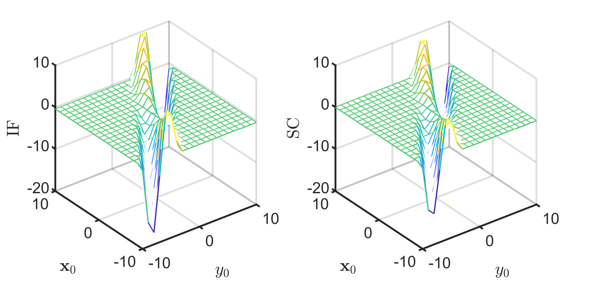
In order to study the local robustness properties of the adaptive $\tau$ -Lasso, we carry out a simulation study on the influence function of the adaptive $\tau$ -Lasso estimator. This allows us to verify the correctness of our results concerning the influence function of the adaptive $\tau$ -Lasso estimator derived in Theorem 7. We run the simulations on a toy one-dimensional dataset as visualizing the influence function becomes difficult in high-dimensional problems. We generate a dataset of $n=1000$ i.i.d observations following the linear model described by equation (2) with $p=1$ where the parameter vector $\boldsymbol{\beta}_{0}=1.5$ . The rows of the regression matrix $\mathbf{X}$ and the noise vector $\mathbf{u}$ are randomly drawn from a Gaussian distribution with zero mean and unit variance. We calculate the influence function via the closed-form expression derived in Theorem 7, given by equation (VI-B4), for the given synthetic data. We then validate the results by plotting the standardized sensitivity curve (SC), which is a finite-sample version of the influence function. We define the standardized sensitivity curve of the estimator $\hat{\theta}$ for a sample of $n$ observations $\mathbf{Z}$ at point $\mathbf{z}_{0}\in\mathscr{Z}_{0}$ as

\text{SC}(\mathbf{z}_{0};\hat{\theta})=\frac{\hat{\theta}(\mathbf{Z},\mathbf{z}_{0})-\hat{\theta}(\mathbf{Z})}{1/(n+1)}.

(37)

We compute the derived influence function and standardized sensitivity curve for a two-dimensional grid of $(y_{0},\mathbf{x}_{[0]})$ with a linear spacing of $1$ , spanning from $-10$ to $10$ along each dimension for $\lambda_{n}=0.1/n$ . We observe from Fig. 3 that the influence function and the standardized sensitivity curve are almost identical and bounded across the plotted space.

Refer to caption — Fig. 3: Plots of influence function (IF) and standardized sensitivity curve (SC) of the adaptive $\tau$ -Lasso estimator as a function of $\mathbf{z}_{0}=(y_{0},\mathbf{x}_{[0]})$ for a one-dimensional toy example with regularization parameter $\lambda_{n}=0.1/n$ . As predicted, the plotted IF and SC are almost identical and bounded across the entire plotted space, which indicates the correctness of our results about the influence function of the adaptive $\tau$ -Lasso estimator derived in Theorem 7.

VII-I When does adaptive $\tau$ -Lasso outperform $\tau$ -Lasso?

Here, we briefly discuss several scenarios where adaptive $\tau$ -Lasso gives superior performance compared to the $\tau$ -Lasso and other considered regularized robust estimators. First, when the true regression coefficients vary greatly in magnitude, the $\tau$ -Lasso tends to overshrink large coefficients and introduces significant bias. In contrast, adaptive $\tau$ -Lasso reduces this bias via an adaptive $\ell_{1}$ -norm penalty. This advantage is demonstrated in Section VII-G. Second, in practical scenarios where good leverage points are present on truly irrelevant predictors, the $\tau$ -Lasso may produce a higher number of false positives. Adaptive $\tau$ -Lasso addresses this problem and reduces the number of false positives. A detailed explanation of this phenomenon can be found in [21], and simulation results demonstrating this behavior are presented in Section S.VI of the Supplemental Material. Third, when truly irrelevant variables are highly correlated with the set of truly relevant variables, the $\tau$ -Lasso may fail to correctly select truly relevant variables or even select too many irrelevant variables. Moreover, adaptive $\tau$ -Lasso can outperform regularized robust regression estimators with convex loss functions, such as LAD-Lasso, particularly in the presence of high-leverage points. Furthermore, in scenarios with a small sample size, adaptive $\tau$ -Lasso shows better predictive and variable selection performance compared to Sparse-LTS, because Sparse-LTS discards a portion of the data to achieve robustness, which adversely impacts the accuracy of the estimation. Note that adaptive $\tau$ -Lasso outperforms $\tau$ -Lasso and the estimators discussed above in the scenarios considered, given that the pilot estimates are reasonably accurate.

VIII Conclusion

This paper introduced the adaptive $\tau$ -Lasso estimator for dealing with high-dimensional data subject to outliers and high-leverage points and discussed its favorable robustness and statistical properties. We established asymptotic theory for consistency of the $\tau$ -Lasso and showed that the adaptive $\tau$ -Lasso possesses the oracle properties. We then analyzed the adaptive $\tau$ -Lasso estimator from a robustness perspective and derived its finite-sample breakdown point and influence function. We studied the performance of the adaptive $\tau$ -Lasso estimator compared with other competing regularized robust estimators through extensive simulations. Our results indicate that even in the presence of contamination, the class of $\tau$ -Lasso estimators, including adaptive $\tau$ -Lasso and $\tau$ -Lasso, performs reliably and achieves either the best performance or matches it with minimal or no performance loss in terms of RMSE/MAD and variable selection for almost all scenarios. The only exception is the oracle estimators, which assume that the true support of parameter vector $\boldsymbol{\beta}_{0}$ is known. These results suggest that the adaptive $\tau$ -Lasso and $\tau$ -Lasso estimators can be effectively utilized for a variety of sparse linear regression problems, particularly in high-dimensional settings and when the data is contaminated by outliers and high-leverage points. It is worth noting that none of the compared estimators has the best performance in all considered scenarios.

References

[1] T. Hastie, R. Tibshirani, and M. Wainwright, Statistical Learning with Sparsity: The Lasso and Generalizations. CRC Press, 2015, vol. 143.
[2] M. J. Wainwright, High-Dimensional Statistics: A Non-Asymptotic Viewpoint. Cambridge University Press, 2019, vol. 48.
[3] K. Slavakis, G. B. Giannakis, and G. Mateos, “Modeling and optimization for big data analytics:(statistical) learning tools for our era of data deluge,” IEEE Signal Processing Magazine, vol. 31, no. 5, pp. 18–31, 2014.
[4] H. Zou and T. Hastie, “Regularization and Variable Selection via the Elastic Net,” Journal of the Royal Statistical Society Series B: Statistical Methodology, vol. 67, no. 2, pp. 301–320, 2005.
[5] H. Zou, “The adaptive lasso and its oracle properties,” Journal of the American Statistical Association, vol. 101, no. 476, pp. 1418–1429, 2006.
[6] R. E. Carrillo, A. B. Ramirez, G. R. Arce, K. E. Barner, and B. M. Sadler, “Robust compressive sensing of sparse signals: a review,” EURASIP Journal on Advances in Signal Processing, vol. 108, pp. 1–17, 2016.
[7] J. Fan, Q. Li, and Y. Wang, “Estimation of High Dimensional Mean Regression in the Absence of Symmetry and Light Tail Assumptions,” Journal of the Royal Statistical Society Series B: Statistical Methodology, vol. 79, no. 1, pp. 247–265, 2016.
[8] H. Wang, G. Li, and G. Jiang, “Robust regression shrinkage and consistent variable selection through the LAD-Lasso,” Journal of Business & Economic Statistics, vol. 25, no. 3, pp. 347–355, 2007.
[9] J. A. Khan, S. Van Aelst, and R. H. Zamar, “Robust linear model selection based on least angle regression,” Journal of the American Statistical Association, vol. 102, no. 480, pp. 1289–1299, 2007.
[10] G. Li, H. Peng, and L. Zhu, “Nonconcave penalized M-estimation with a diverging number of parameters,” Statistica Sinica, vol. 21, no. 1, pp. 391–419, 2011.
[11] S. Lambert-Lacroix and L. Zwald, “Robust regression through the Huber’s criterion and adaptive lasso penalty,” Electronic Journal of Statistics, vol. 5, pp. 1015–1053, 2011.
[12] ——, “The adaptive BerHu penalty in robust regression,” Journal of Nonparametric Statistics, vol. 28, no. 3, pp. 487–514, 2016.
[13] Q. Sun, W.-X. Zhou, and J. Fan, “Adaptive Huber regression,” Journal of the American Statistical Association, vol. 115, no. 529, pp. 254–265, 2020.
[14] J. Fan, Y. Fan, and E. Barut, “Adaptive robust variable selection,” The Annals of Statistics, vol. 42, no. 1, pp. 324–351, 2014.
[15] J. Bradic, J. Fan, and W. Wang, “Penalized composite quasi-likelihood for ultrahigh dimensional variable selection,” Journal of the Royal Statistical Society Series B: Statistical Methodology, vol. 73, no. 3, pp. 325–349, 2011.
[16] J. Bradic, “Robustness in sparse high-dimensional linear models: Relative efficiency and robust approximate message passing,” Electronic Journal of Statistics, vol. 10, no. 2, pp. 3894–3944, 2016.
[17] J. Fan, H. Liu, Q. Sun, and T. Zhang, “I-LAMM for sparse learning: Simultaneous control of algorithmic complexity and statistical error,” The Annals of Statistics, vol. 46, no. 2, pp. 814–841, 2018.
[18] P.-L. Loh, “Statistical consistency and asymptotic normality for high-dimensional robust M-estimators,” The Annals of Statistics, vol. 45, no. 2, pp. 866–896, 2017.
[19] E. Smucler and V. J. Yohai, “Robust and sparse estimators for linear regression models,” Computational Statistics & Data Analysis, vol. 111, pp. 116–130, 2017.
[20] R. A. Maronna, R. D. Martin, V. J. Yohai, and M. Salibián-Barrera, Robust Statistics: Theory and Methods (with R), 2nd ed. John Wiley & Sons, 2019.
[21] D. Kepplinger, “Robust variable selection and estimation via adaptive elastic net S-estimators for linear regression,” Computational Statistics & Data Analysis, vol. 183, p. 107730, 2023.
[22] G. V. C. Freue, D. Kepplinger, M. Salibián-Barrera, and E. Smucler, “Robust elastic net estimators for variable selection and identification of proteomic biomarkers,” The Annals of Applied Statistics, vol. 13, no. 4, pp. 2065–2090, 2019.
[23] M. Martinez-Camara, M. Muma, A. M. Zoubir, and M. Vetterli, “A new robust and efficient estimator for ill-conditioned linear inverse problems with outliers,” in 2015 IEEE International Conference on Acoustics, Speech and Signal Processing (ICASSP). IEEE, 2015, pp. 3422–3426.
[24] M. Martinez-Camara, M. Muma, B. Bejar, A. M. Zoubir, and M. Vetterli, “The regularized tau estimator: A robust and efficient solution to ill-posed linear inverse problems,” May 2016. [Online]. Available: https://arxiv.org/pdf/1606.00812
[25] P.-L. Loh and M. J. Wainwright, “Support recovery without incoherence: A case for nonconvex regularization,” The Annals of Statistics, vol. 45, no. 6, pp. 2455–2482, 2017.
[26] V. J. Yohai and R. H. Zamar, “High breakdown-point estimates of regression by means of the minimization of an efficient scale,” Journal of the American Statistical Association, vol. 83, no. 402, pp. 406–413, 1988.
[27] ——, “High Breakdown-Point Estimates of Regression by Means of Minimization of an Efficient Scale,” Department of Statistics, University of Washington, Seattle, Tech. Rep. No. 84, April 1986.
[28] J. Shao, Mathematical Statistics. Springer Science & Business Media, 2003.
[29] H. Zou and H. H. Zhang, “On the adaptive elastic-net with a diverging number of parameters,” The Annals of Statistics, vol. 37, no. 4, pp. 1733 – 1751, 2009.
[30] A. M. Zoubir, V. Koivunen, E. Ollila, and M. Muma, Robust Statistics for Signal Processing. Cambridge, UK: Cambridge University Press, 2018.
[31] E. Mozafari-Majd and V. Koivunen, “Two-stage robust and sparse distributed statistical inference for large-scale data,” IEEE Transactions on Signal Processing, vol. 70, pp. 5351–5365, 2022.
[32] A. W. Van der Vaart, Asymptotic Statistics, ser. Cambridge Series in Statistical and Probabilistic Mathematics. Cambridge University Press, 1998.
[33] M. Avella-Medina, “Influence functions for penalized M-estimators,” Bernoulli, vol. 23, no. 4B, pp. 3178–3196, 2017.
[34] R. A. Maronna, “Robust ridge regression for high-dimensional data,” Technometrics, vol. 53, no. 1, pp. 44–53, 2011.
[35] A. Alfons, C. Croux, and S. Gelper, “Sparse least trimmed squares regression for analyzing high-dimensional large data sets,” The Annals of Applied Statistics, vol. 7, no. 1, pp. 226–248, 2013.
[36] X. Wang, Y. Jiang, M. Huang, and H. Zhang, “Robust variable selection with exponential squared loss,” Journal of the American Statistical Association, vol. 108, no. 502, pp. 632–643, 2013.
[37] R. Tibshirani, “Regression shrinkage and selection via the lasso,” Journal of the Royal Statistical Society. Series B (Methodological), vol. 58, no. 1, pp. 267–288, 1996.
[38] J. Fan and H. Peng, “Nonconcave penalized likelihood with a diverging number of parameters,” The Annals of Statistics, vol. 32, no. 3, pp. 928–961, 2004.
[39] T. Hastie, R. Tibshirani, and J. Friedman, The Elements of Statistical Learning, ser. Springer Series in Statistics. New York, NY, USA: Springer New York Inc., 2009.

See pages 1-28 of Supp_Mat_Final_Second_Sumbission.pdf

The Adaptive τ\tau-Lasso: Robustness and Oracle Properties

Abstract

Index Terms:

I Introduction

I-A Related work

I-B Organization

II Notation

List of Notations

III Data Model

IV The Adaptive τ\tau-Lasso

IV-A Definition

IV-B Computation of the adaptive τ\tau-Lasso estimates

IV-C Choice of ρ\rho-function

IV-D Choice of pilot estimator

V Consistency and Oracle Properties

VI Robustness

VI-A Finite-sample breakdown point

VI-B Influence function (IF)

VI-B1 Definition

VI-B2 Regularized M-estimators

VI-B3 Necessary mathematical notations

VI-B4 Theorems on the influence function of adaptive τ\tau-Lasso estimator

VII Simulation results

VII-A Standardization of data

VII-B Choice of tuning constants c0c_{0} and c1c_{1}

VII-C Simulation scenarios

VII-D Competing state-of-the-art methods

VII-E Results

VII-F RMSE under contamination

VII-G A remedy for overshrinkage in τ\tau-Lasso

VII-H The empirical validation of the influence function

VII-I When does adaptive τ\tau-Lasso outperform τ\tau-Lasso?

VIII Conclusion

References

The Adaptive $\tau$ -Lasso: Robustness and Oracle Properties

IV The Adaptive $\tau$ -Lasso

IV-B Computation of the adaptive $\tau$ -Lasso estimates

IV-C Choice of $\rho$ -function

VI-B4 Theorems on the influence function of adaptive $\tau$ -Lasso estimator

VII-B Choice of tuning constants $c_{0}$ and $c_{1}$

VII-G A remedy for overshrinkage in $\tau$ -Lasso

VII-I When does adaptive $\tau$ -Lasso outperform $\tau$ -Lasso?