跳到论文正文
W Papers独立论文阅读器 arXiv:2304.09019 论文正文 计算阅读时间 · 0%
引用这篇论文根据当前论文元数据生成,正式投稿前建议核对。


License: CC BY 4.0
arXiv:2304.09019v1 [cs.IT] 18 Apr 2023

Hardware-Impaired Rician-Faded Cell-Free Massive MIMO Systems With Channel Aging

Venkatesh Tentu    Dheeraj N Amudala    Anish Chattopadhyay    Rohit Budhiraja Thanks: The authors are with the Dept. of Electrical Engineering, IIT Kanpur, India. email: {tentu, dheeraja, anishchat20, rohitbr}@iitk.ac.in. A part of this work is accepted for presentation in IEEE International Conference on Communications 2023.
Abstract

We study the impact of channel aging on the uplink of a cell-free (CF) massive multiple-input multiple-output (mMIMO) system by considering i) spatially-correlated Rician-faded channels; ii) hardware impairments at the access points and user equipments (UEs); and iii) two-layer large-scale fading decoding (LSFD). We first derive a closed-form spectral efficiency (SE) expression for this system, and later propose two novel optimization techniques to optimize the non-convex SE metric by exploiting the minorization-maximization (MM) method. The first one requires a numerical optimization solver, and has a high computation complexity. The second one with closed-form transmit power updates, has a trivial computation complexity. We numerically show that i) the two-layer LSFD scheme effectively mitigates the interference due to channel aging for both low- and high-velocity UEs; and ii) increasing the number of AP antennas does not mitigate the SE deterioration due to channel aging. We numerically characterize the optimal pilot length required to maximize the SE for various UE speeds. We also numerically show that the proposed closed-form MM optimization yields the same SE as that of the first technique, which requires numerical solver, and that too with a much reduced time-complexity.

Index Terms:
Cell-free, channel aging, hardware impairments, minorization-maximization (MM), Rician fading.

I Introduction

Cell-free (CF) massive multiple-input multiple output (mMIMO) is being investigated as a key technology for beyond fifth-generation wireless systems due to its high spectral efficiency (SE) and improved coverage [1]. A CF mMIMO system consists of a large number of access points (APs) which are randomly deployed over a large coverage area, and are connected to a central processing unit (CPU) via high-speed fronthaul links. The APs cooperate via these fronthaul links to mitigate the inter-user interference (IUI) caused due to multiple user equipments (UEs) being served on the same time-frequency resource [1, 2]. Initial CF mMIMO works commonly considered single layer decoding (SLD) schemes, wherein APs individually combine their respective receive signals using the locally-estimated channel information, while the CPU handle only data detection [1, 2]. Ngo et al. in [1] investigated the SE gains provided by a CF mMIMO system with SLD, over its conventional small-cell counterpart. The authors in [2] proposed scalable combiners and precoders for a spatially-correlated Rayleigh-faded CF mMIMO system with SLD, and showed that they outperform conventional maximum ratio processing. We know that fifth generation (5G) cellular networks have recently been deployed. The channel models considered to evaluate different technologies for 5G systems e.g., mMIMO, contain line of sight (LoS) components, along with the non LoS (NLoS) one[3]. This makes the channel Rician distributed.

Further, the local SLD techniques, despite having a low implementation complexity, fail to effectively suppress the IUI. This can be improved by performing the second level of combining at the CPU, referred to as the large-scale fading decoding (LSFD) [4, 5, 6]. The key difference between LSFD and SLD receivers is that the former requires additional statistical channel parameters such as large-scale fading coefficients at the CPU. These large-scale fading parameters remain constant over multiple coherence intervals, and thus can be easily made available at the CPU [4, 5, 6]. Ozdogan et al. in [4] showed the improved SE gains obtained due to LSFD for a CF mMIMO system with spatially-correlated Rician-faded channels. Demir et al. in [5] maximized the minimum SE of a wireless-powered CF mMIMO system by considering LSFD and the spatially-correlated Rician-faded channels. Zhang et al. in [6] proposed local zero forcing combiners for an uncorrelated CF mMIMO system, and then integrated these combiners with LSFD, and investigated their SE.

Majority of CF mMIMO works, including the aforementioned ones in [1, 2, 4, 5, 6], considered a block fading channel model, wherein the channel remains constant over a coherence interval. The 5G cellular systems are designed for a UE speed of up to 500500 km/h, whose channel then continuously varies with time [7]. The channel estimated by the APs, consequently, become outdated with time [8, 9]. This channel aging phenomenon can drastically degrade the gains accrued by CF mMIMO technology. The authors in [9, 10, 11, 12] and [13, 14, 15] recently investigated the effect of channel aging on cellular and CF mMIMO systems, respectively. The authors in [9] derived asymptotic power scaling laws which showed the detrimental effect of channel aging on a single-cell correlated Rayleigh-faded mMIMO system. The authors in [10, 11] proposed a machine-learning-based channel predictor for a single-cell mMIMO system with channel aging, which could be used for both uplink and downlink systems. Papazafeiropoulos et al. in [12] analyzed the outage probability of a multi-cell mMIMO system and showed that its preferred to have massive number of antennas under channel aging conditions. Chopra et. al in [13] showed that the impact of channel aging is higher on a CF mMIMO system than on a cellular mMIMO system. This work, however, considered uncorrelated Rayleigh-faded channels and local SLD scheme at the APs. Zheng et. al in [14] and [15] analyzed the effect of channel aging in a CF mMIMO system with LSFD, for uncorrelated and correlated Rayleigh fading channels, respectively. The authors in [15] also proved that the CF mMIMO system is more robust to channel aging than a small-cell system.

The above CF mMIMO works [4, 5, 6, 13, 14, 15] assumed high-quality radio frequency (RF) transceivers and high-resolution analog-to-digital converters (ADCs)/digital-to-analog converters (DACs) at the APs and UEs. The RF transceiver chips used to design 5G cellular system, and its evolved CF mMIMO systems have inherent hardware distortion, which is commonly characterized using the error vector magnitude (EVM) metric. It is usually specified in the device data sheet [16]. The effect of hardware distortion caused by the low-cost hardware can be suppressed by using the calibration schemes and the compensation algorithms, but the residual impairments still remains [17, 18, 19, 20, 21]. The impact of these residual impairments on CF mMIMO systems should be further studied. Masoumi et al. in [17] analyzed the effect of hardware-impairments in a CF mMIMO system with uncorrelated Rayleigh-faded channels. The authors in [18] derived an approximate SE expression for a spatially-correlated Rayleigh-faded CF mMIMO system with hardware impairments. Tentu et. al in [19] investigated the SE of an unmanned aerial vehicle enabled CF mMIMO system with RF impairments and spatially-correlated Rician channels. All these works considered only local SLD schemes, and also ignored channel aging in their analysis. Zhang et al. in [20] analyzed the SE of a hardware-impaired CF mMIMO system with LSFD, and showed that the hardware distortion non-trivially impacts the LSFD performance. This work, however, ignored channel aging. The authors in [21] investigated the joint impact of hardware impairments and channel aging for a CF mMIMO system, but only for uncorrelated Rayleigh channels, and that too without LSFD.

Practical CF mMIMO systems, to reduce the energy consumption and implementation costs, also employ low-resolution ADC/DACs [22, 23, 24]. The authors in [22, 23, 24] studied the effect of low-resolution ADCs in CF mMIMO systems. Zhang et. al in [22] analyzed the SE of spatially-uncorrelated Rayleigh-faded CF mMIMO system with low-resolution ADC/DACs, and showed its improved energy efficiency over high-resolution ADC/DACs. Zhang et. al in [23] investigated the uplink and downlink SE of an uncorrelated Rician-faded CF mMIMO system with low-resolution ADCs at the APs. Hu et. al in [24] investigated the asymptotic SE of an uncorrelated Rayleigh-faded CF mMIMO system, and showed that the SE is mainly limited by the UE ADC resolution, when low-resolution ADCs are used at both APs and UEs. Low resolution ADC/DACs improve the energy efficiency by reducing the power consumption, but also cause non-negligible SE loss due to coarse quantization. To alleviate this problem, the authors in [25, 26] considered a mixed-ADC architecture, wherein one fraction of AP antennas has a high-resolution ADCs, while the other has low-resolution. Zhang et. al in [25] and [26] investigated the SE of a CF mMIMO system with mixed-ADC architecture at the APs by considering spatially-uncorrelated Rayleigh- and Rician-fading respectively, and showed its superiority over its low-resolution counterpart.

Recently, the authors in [27, 28] proposed a dynamic ADC architecture and derived closed-form SE expressions for CF mMIMO with spatially-correlated Rayleigh channels. The dynamic ADC architecture offers the flexibility to tune the ADC resolution of each AP antenna. This provides system designers with extra degrees-of-freedom for system design and optimization. References [22, 23, 24, 25, 26, 27, 28] considered a local SLD scheme and investigated the effect of low-/mixed-/dynamic-resolution ADCs alone. These works ignored RF impairments and channel aging. Also, the existing works [23, 19, 26] modeled the Rician fading channel with a static line-of-sight phase. A small change in the UE location induces significant phase-shift in the LoS path. The authors in [4, 5] modeled these phase-shifts as a uniformly distributed random variable, and derived closed-form SE expression for a CF mMIMO system, but without considering channel-aging, and hardware impairments. It is crucial to analyze the joint effect of RF impairments and ADC/DAC quantization in the presence of channel aging and Rician phase-shifts, which is a crucial gap in the existing CF mMIMO literature. The current work fills this gap, by analyzing a CF mMIMO system with two-layer LSFD, channel aging, Rician phase-shifts, low-cost RF chains and dynamic ADC architecture.

We next summarize in Table I the relevant CF mMIMO literature focusing on LSFD, channel aging, RF and ADC hardware impairments and spatially-correlated Rician faded channels with phase-shifts. We infer from Table I that the existing correlated Rician-faded CF mMIMO literature has not yet investigated the: i) SE with channel aging and two-stage LSFD; ii) RF impairments and dynamic ADC architecture; and iii) sum SE optimization. Additionally, for Rayleigh channels, the CF mMIMO LSFD literature, has not investigated the i) SE with channel aging and non-ideal hardware and; ii) sum SE optimization.

Table I: Summary of CF mMIMO literature focusing on LSFD and Channel aging.
Ref. LSFD Channel aging Rayleigh/ Rician Correlation RF impairments ADC architecture Optimization
[4] ✓ ✗ Rician ✗ ✗ ideal ✗
[13] ✗ ✓ Rayleigh ✗ ✗ ideal ✗
[15] ✓ ✓ Rayleigh ✓ ✗ ideal ✗
[20] ✓ ✗ Rayleigh ✗ ✓ ideal ✗
[21] ✗ ✓ Rayleigh ✗ ✓ ideal max-min SE
[23] ✗ ✗ Rician ✗ ✗ low-resolution weighted max-min SE
[26] ✗ ✗ Rician ✗ ✗ mixed-resolution ✗
[27] ✗ ✗ Rayleigh ✓ ✗ dynamic-resolution ✗
Pr. ✓ ✓ Rician ✓ ✓ dynamic-resolution sum-SE

The main contributions of the current work address these gaps as follows:

  • •

    We consider a spatially-correlated Rician-faded CF mMIMO system with channels aging, and investigate the impact of dynamic ADC architecture and low-cost hardware-impaired RF chains. We also consider the two-layer LSFD, and derive a closed-form SE expression by addressing the derivation difficulties caused by the combined modelling of channel aging, RF impairments, dynamic ADC architecture and spatially-correlated Rician channels.

  • •

    We use the derived closed-form SE expression to maximize the non-convex SE metric by optimizing the UE transmit powers and the LSFD coefficients, which is the second contribution of this work. We propose two optimal power allocation schemes using minorization-maximization (MM) technique, which iteratively maximizes the convex surrogate of the non-convex objective [29]. We propose a novel convex surrogate function, and analytically show that it satisfies the desirable surrogacy properties [29]. This approach, however, has a high computation complexity as it requires off-the-shelf optimization solvers [29]. We next design a low-complexity practically-implementable power allocation technique by using the Lagrangian dual transform technique [30]. This enables us in designing the closed-form transmit power update, which has a trivial computational complexity. It is extremely useful for designing optimal power for practical CF mMIMO systems with channel aging.

  • •

    We show that LSFD can effectively mitigate the detrimental effects of i) channel aging for both low and high UE velocities; and ii) IUI for low-velocity UEs but not for high-velocity UEs. We also show that the increased number of AP antennas cannot mitigate the SE degradation due to channel aging.

The rest of the paper is organized as follows. Section II discusses the channel model, uplink channel estimation and data transmission, and LSFD for the proposed hardware-impaired CF mMIMO system with channel aging. Section III derives and analyzes the closed-form SE expression for the aforementioned system. Section IV proposes two optimal power allocation schemes to optimize SE. Section V first numerically validates the efficacy of the derived closed-form SE. It then investigates the effect of channel aging and LSFD on the SE. It then compares the complexity of the proposed optimization techniques. Section VI finally concludes the paper.

Notations: Bold-faced lower- and upper-case alphabet denote vectors and matrices, respectively. Superscripts (⋅)∗(\cdot)^{*}, (⋅)T(\cdot)^{T}, (⋅)H(\cdot)^{H} and (⋅)−1(\cdot)^{-1} denote the conjugate, transpose, conjugate transpose and inverse, respectively, and 𝔼​{⋅}\mathbb{E}\{\cdot\} is the expectation operator. Trace and diagonal of a matrix 𝐗\mathbf{X} are denoted as tr​(𝐗)\text{tr}(\mathbf{X}) and diag​(𝐗)\text{diag}(\mathbf{X}), respectively. Also, ∥⋅∥\|\cdot\| is the Euclidean 2-norm, |⋅||\cdot| is the absolute value and real​{⋅}\text{real}\{\cdot\} is the real-part of the argument. The notation 𝒞​𝒩​(𝟎,𝐈)\mathcal{CN}(\mathbf{0},\mathbf{I}) denotes a complex circular Gaussian random vector with zero mean and covariance matrix 𝐈\mathbf{I}.

II System Model

We consider the uplink of a CF mMIMO system with MM multi-antenna APs and KK single-antenna UEs. Each AP has NN antennas. We assume, similar to [5, 24], that the APs are randomly distributed over a large geographical area, and are connected to a CPU via high-speed fronthaul links. To reduce the system hardware cost and power consumption, APs and UEs are equipped with low-cost hardware-impaired RF chains. Further, the APs have a dynamic-resolution ADC architecture, wherein each AP antenna can be connected to a different resolution ADC. This is unlike [22, 25, 26], which assume that the ADCs either have a low or a mixed resolution. The UEs are designed using low-resolution DACs. In correlated Rician-faded cell-free mMIMO systems, the channel does not harden. For high speed UEs, the channel will age. To investigate channel aging effect, we consider, as shown in Fig. 1, a resource block of length τc\tau_{c} time instants.

Figure 1: Structure of resource block of length τc\tau_{c} time instants.

The channel remains constant for a time instant, and varies across time instants in a correlated manner. This temporal correlation is modeled later using Jake’s model [15]. We also assume that each resource block is divided into uplink training and data transmission intervals of length τp\tau_{p} and (τc−τp)(\tau_{c}-\tau_{p}) time instants, respectively. We next model the UE-AP channel.

II-A Channel model

The channel from the kkth UE to the mmth AP at the λ\lambdath time instant is denoted as 𝐡m​k​[λ]\mathbf{h}_{mk}[\lambda]. Due to dense AP deployment, the channel 𝐡m​k​[λ]\mathbf{h}_{mk}[\lambda] contains both LoS and NLoS paths. It, therefore, has a Rician probability density function (pdf), and is modeled as follows [4]:

𝐡m​k​[λ]=𝐡¯m​k​ej​ϕm​kλ+𝐑m​k12​𝐡~m​k​[λ].\displaystyle\!\!\!\mathbf{h}_{mk}[\lambda]=\bar{\mathbf{h}}_{mk}e^{j\phi_{mk}^{\lambda}}\!+\!\mathbf{R}_{mk}^{\frac{1}{2}}\tilde{\mathbf{h}}_{mk}[\lambda]. (1)

Here 𝐡¯m​k=Km​k​βm​kKm​k+1​𝐡˘m​k\bar{\mathbf{h}}_{mk}=\sqrt{\frac{\!K_{mk}\beta_{mk}}{\!K_{mk}+1}}\breve{\mathbf{h}}_{mk}, 𝐑m​k=βm​kKm​k+1​𝐑˘m​k\mathbf{R}_{mk}\!=\frac{\beta_{mk}}{\!K_{mk}\!+\!1}\breve{\mathbf{R}}_{mk}. The term Km​kK_{mk} is the Rician factor, and βm​k\beta_{mk} is the large-scale fading coefficient. The LoS term 𝐡˘m​k\breve{\mathbf{h}}_{mk} is modeled as 𝐡˘m​k=[1,ej​ψm​k,⋯,ej⁡(M−1)​ψm​k]T\breve{\mathbf{h}}_{mk}=[1,e^{j\psi_{mk}},\cdots,e^{j(M-1)\psi_{mk}}]^{T}, where ψm​k\psi_{mk} is the angle of arrival from the kkth UE to the mmth AP. The term, 𝐡~m​k​[λ]\tilde{\mathbf{h}}_{mk}[\lambda], with pdf 𝒞​𝒩​(𝟎,𝐈N)\mathcal{CN}(\mathbf{0},\mathbf{I}_{N}) models the small-scale NLoS fading. The term 𝐑˘m​k\breve{\mathbf{R}}_{mk} is the spatial correlation matrix. The LoS phase-shift ϕm​kλ\phi_{mk}^{\lambda} at the λ\lambdath instant is uniformly distributed between [−π,π][-\pi,\pi]. The long-term channel statistics i.e., 𝐡¯m​k\bar{\mathbf{h}}_{mk}, βm​k\beta_{mk} and 𝐑m​k\mathbf{R}_{mk}, remain constant over a resource block and, similar to [4], are assumed to be perfectly known at the AP. Most of the Rician CF works e.g., [31, 32, 19], assume that the LoS phase-shift ϕm​kλ\phi_{mk}^{\lambda} is static. A slight change in UEs position, however, can radically modify the phase. It is, thus, crucial to consider a dynamic phase-shift ϕm​kλ\phi_{mk}^{\lambda} in the Rician channel to practically model it [4]. We accordingly, similar to [4], assume that ϕm​kλ\phi_{mk}^{\lambda} varies as frequently as small-scale fading, and that the AP is unaware of it. As an AP does not have the prior knowledge of ϕm​kλ\phi_{mk}^{\lambda}, it estimates the channel 𝐡m​k\mathbf{h}_{mk}, without its knowledge.

As discussed earlier, due to UEs mobility, the AP-UE channel in a resource block varies across time instants, which causes channel aging [15]. To analyze its effect, we model the channel 𝐡m​k​[n]\mathbf{h}_{mk}[n] at the nnth time instant 1≤n≤τc1\leq n\leq\tau_{c}, as a combination of the channel 𝐡m​k​[λ]\mathbf{h}_{mk}[\lambda] at the time instant λ\lambda, and the innovation component as follows [14, 15]:

𝐡m​k​[n]=ρk​[λ−n]​𝐡m​k​[λ]+1−ρk2​[λ−n]​(𝐡¯m​k​ej​ϕm​kn+𝐟m​k​[n]).\displaystyle\mathbf{h}_{mk}[n]=\rho_{k}[\lambda-n]\mathbf{h}_{mk}[\lambda]+\sqrt{1-\rho_{k}^{2}[\lambda-n]}\Big(\bar{\mathbf{h}}_{mk}e^{j\phi_{mk}^{n}}+\mathbf{f}_{mk}[n]\Big). (2)

The temporal correlation ρk​[λ−n]\rho_{k}[\lambda-n], based on the Jake’s model [15], is given as ρk​[λ−n]=J0​(2​π​fd,i​Ts​(λ−n))\rho_{k}[\lambda-n]=J_{0}(2\pi f_{d,i}T_{s}(\lambda-n)). Here J0​(⋅)J_{0}(\cdot) is the zeroth-order Bessel function, and TsT_{s} is the sampling time. The term fd,i=(vk​fc)/cf_{d,i}=(v_{k}f_{c})/c is the Doppler spread, with vkv_{k}, fcf_{c} and cc being the user velocity, carrier frequency and the velocity of light, respectively. The innovation component 𝐟m​k​[n]\mathbf{f}_{mk}[n] is independent of the channel at the time instant λ\lambda i.e., 𝐡m​k​[λ]{\mathbf{h}}_{mk}[\lambda], and has a pdf 𝒞​𝒩​(𝟎,𝐑m​k)\mathcal{CN}(\mathbf{0},\mathbf{R}_{mk}) [15].

II-B Uplink training

Recall that the uplink training phase consists of τp\tau_{p} time instants. The kkth UE, similar to [15], transmits its pilot signal p~k​ϕk​[tk]\sqrt{\tilde{p}_{k}}\phi_{k}[t_{k}] at the time instant tk⊂{1,…,τp}t_{k}\subset\{1,\dots,\tau_{p}\}. Here |ϕk​[tk]|2=1|\phi_{k}[t_{k}]|^{2}=1. We assume that the uplink training duration τp<K\tau_{p}<K. The number of UEs transmitting pilot at a particular time instant is more than one, which causes pilot contamination [4]. The set of UEs that transmit pilots at the time instant tkt_{k} is denoted as 𝒫k\mathcal{P}_{k}. The kkth UE feeds its pilot signal to the low-resolution DAC, which distorts it. This distortion is commonly analyzed using Bussgang model [33]. The distorted DAC output, based on the Bussgang model, is:

sDAC,kp​[tk]=Q⁡(p~k​ϕk​[tk])=αd,k​p~k​ϕk​[tk]+υDAC,kp​[tk].\displaystyle s_{\text{DAC},k}^{p}[t_{k}]=Q(\sqrt{\tilde{p}_{k}}\phi_{k}[t_{k}])=\alpha_{d,k}\sqrt{\tilde{p}_{k}}\phi_{k}[t_{k}]+\upsilon^{p}_{\text{DAC},k}[t_{k}]. (3)

Here αd,k=−ιd,k\alpha_{d,k}=1\!-\iota_{d,k} with ιd,k\iota_{d,k} being the DAC distortion factor. The term υDAC,kp​[tk]\upsilon^{p}_{\text{DAC},k}[t_{k}] is zero-mean DAC quantization noise, which is uncorrelated with the input pilot signal, and has a variance αd,k​(−αd,k)​p~k​𝔼​{|ϕk​[tk]|2}\alpha_{d,k}(1\!-\!\alpha_{d,k})\tilde{p}_{k}\mathbb{E}\big\{|\phi_{k}[t_{k}]|^{2}\big\} [4]. The kkth UE DAC output signal sDAC,kp​[tk]s_{\text{DAC},k}^{p}[t_{k}] is fed to its hardware- impaired RF chain, which adds a distortion term ξRF,kp​[tk]\xi_{\text{RF},k}^{p}[t_{k}] [34]. The effective uplink pilot signal is, therefore, given as sRF,kp​[tk]=sDAC,kp​[tk]+ξRF,kp​[tk]s_{\text{RF},k}^{p}[t_{k}]=s_{\text{DAC},k}^{p}[t_{k}]+\xi_{\text{RF},k}^{p}[t_{k}]. The distortion ξRF,kp​[tk]\xi_{\text{RF},k}^{p}[t_{k}] is independent of the input signal, and has a pdf 𝒞​𝒩​(0,κt,k2​(𝔼⁡{sDAC,kp​[tk]​(sDAC,kp​[tk])H}))\mathcal{CN}\big(0,\kappa_{t,k}^{2}\big(\mathbb{E}\{s^{p}_{\text{DAC},k}[t_{k}](s_{\text{DAC},k}^{p}[t_{k}])^{H}\}\big)\big) [34]. The term κt,k\kappa_{t,k} in the pdf models the UE transmit EVM [34]. At the tkt_{k} time instant, the mmth AP receives at its antennas, the sum of pilot signals transmitted by UEs in the set 𝒫k\mathcal{P}_{k} i.e.,

𝐲mp​[tk]=∑i∈𝒫k𝐡m​i​[tk]​sRF,ip​[tk].\displaystyle\mathbf{y}_{m}^{p}[t_{k}]=\sum\limits_{i\in\mathcal{P}_{k}}\mathbf{h}_{mi}[t_{k}]s_{\text{RF},i}^{p}[t_{k}]. (4)

To reduce the system cost, the APs are designed using hardware-impaired RF chains and a dynamic-ADC architecture, which enables us to vary the resolution of each ADC from 11 to a maximum of DD bits. The mmth AP feeds the above pilots signal received at its antenna to the hardware-impaired RF chains, whose distorted output, based on the EVM model, is [34]:

𝐲RF,mp​[tk]=𝐲mp​[tk]+𝜼RF,mp​[tk]+𝐳mp​[tk].\displaystyle\mathbf{y}_{\text{RF},m}^{p}[t_{k}]=\mathbf{y}_{m}^{p}[t_{k}]+\boldsymbol{\eta}_{\text{RF},m}^{p}[t_{k}]+\mathbf{z}_{m}^{p}[t_{k}]. (5)

The term 𝜼RF,mp​[tk]\boldsymbol{\eta}_{\text{RF},m}^{p}[t_{k}], with pdf 𝒞​𝒩​(𝟎,κr,m2​𝐖m​[tk])\mathcal{CN}(\boldsymbol{0},\kappa_{r,m}^{2}\mathbf{W}_{m}[t_{k}]), models the RF hardware distortion. The term κr,m2\kappa_{r,m}^{2} is the AP receiver EVM and 𝐖m​[tk]=diag​(𝔼⁡{𝐲mp​[tk]​(𝐲mp​[tk])H|𝐡m​k​[tk]})\mathbf{W}_{m}[t_{k}]=\text{diag}\big(\mathbb{E}\big\{\mathbf{y}_{m}^{p}[t_{k}](\mathbf{y}_{m}^{p}[t_{k}])^{H}\big|\mathbf{h}_{mk}[t_{k}]\big\}\big). Note that the receive hardware impairment is proportional to the power of UEs transmit signals [34]. The vector 𝐳m​[tk]\mathbf{z}_{m}[t_{k}], with pdf 𝒞​𝒩​(𝟎,𝐈N)\mathcal{CN}(\boldsymbol{0},\mathbf{I}_{N}), is the additive white Gaussian noise (AWGN) at the mmth AP. The RF chain output is then fed to the dynamic-resolution ADCs, which distort it by adding quantization noise. The distorted ADCs output, based on the Bussgang model [33], is given as

𝐲ADC,mp​[tk]=𝐀m​𝐲RF,mp​[tk]+𝐧ADC,mp​[tk]=𝐀m​(𝐲mp​[tk]+𝜼RF,mp​[tk]+𝐳mp​[tk])+𝐧ADC,mp​[tk].\displaystyle\mathbf{y}_{\text{ADC},m}^{p}[t_{k}]=\mathbf{A}_{m}\mathbf{y}_{\text{RF},m}^{p}[t_{k}]+{\mathbf{n}^{p}_{\text{ADC},m}}[t_{k}]=\mathbf{A}_{m}\big(\mathbf{y}_{m}^{p}[t_{k}]+\boldsymbol{\eta}^{p}_{\text{RF},m}[t_{k}]+\mathbf{z}^{p}_{m}[t_{k}]\big)+{\mathbf{n}^{p}_{\text{ADC,m}}}[t_{k}]. (6)

The matrix 𝐀m=diag​(1−ιm,n,⋯,1−ιm,n)\mathbf{A}_{m}=\text{diag}(1-\iota_{m,n},\cdots,1-\iota_{m,n}), where ιm,n\iota_{m,n} is the ADC distortion factor [33]. The zero-mean additive ADC quantization noise 𝐧ADC,mp​[tk]{\mathbf{n}^{p}_{\text{ADC},m}}[t_{k}] is uncorrelated with 𝐲RF,mp​[tk]\mathbf{y}_{\text{RF},m}^{p}[t_{k}]. It has a covariance of 𝐁m​diag​(𝔼⁡{𝐲RF,mp​[tk]​(𝐲RF,mp​[tk])H|𝐡m​k​[tk]})\mathbf{B}_{m}\text{diag}\big(\mathbb{E}\big\{\mathbf{y}_{\text{RF},m}^{p}[t_{k}](\mathbf{y}_{\text{RF},m}^{p}[t_{k}])^{H}\big|\mathbf{h}_{mk}[t_{k}]\big\}\big) with 𝐁m=𝐀m​(𝐈N−𝐀m)\mathbf{B}_{m}=\mathbf{A}_{m}(\mathbf{I}_{N}-\mathbf{A}_{m}) [33]. The existing CF mMIMO literature [35, 20, 17, 21, 24, 22, 23], except [27], has not investigated the dynamic-resolution ADC architecture with different diagonal elements of 𝐀m\mathbf{A}_{m} i.e., ιm,p≠ιm,q\iota_{m,p}\neq\iota_{m,q} for p≠qp\neq q. It significantly complicates the SE analysis and derivation, when compared with [35, 20, 17, 21, 24, 22, 23], which considers either low- or mixed-ADC architecture at the APs. Xiong et. al in [27] considered a CF mMIMO system with dynamic-ADC architecture, but with correlated Rayleigh fading channels and ideal RF chains at the APs and UEs. The current work, in contrast, studies the dynamic ADC/DAC architecture for a CF mMIMO system with i) low-cost RF chains; ii) spatially-correlated Rician channel with phase-shifts; and iii) channel aging. The proposed architecture is generic, and reduces to its low-resolution and mixed-resolution counterparts by choosing 𝐀m=(1−ιm)​𝐈N\mathbf{A}_{m}=(1-\iota_{m})\mathbf{I}_{N} and 𝐀m=blkdiag​{(1−ιm)​𝐈γ,𝐈N−γ}\mathbf{A}_{m}=\text{blkdiag}\{(1-\iota_{m})\mathbf{I}_{\gamma},\mathbf{I}_{N-\gamma}\} with 0≤γ≤N0\leq\gamma\leq N, respectively.

We next substitute expression of 𝐲mp​[tk]\mathbf{y}_{m}^{p}[t_{k}] from (4) in (6), and re-express 𝐲ADC,mp​[tk]\mathbf{y}_{\text{ADC},m}^{p}[t_{k}] as

𝐲ADC,mp​[tk]\displaystyle\mathbf{y}_{\text{ADC},m}^{p}[t_{k}] =∑i∈𝒫k𝐀m​(𝐡m​i​[tk]​(αd,i​p~i+υDAC,ip​[tk]+ξRF,ip​[tk])+𝜼RF,mp​[tk]+𝐳mp​[tk])+𝐧ADC,mp​[tk].\displaystyle=\!\sum_{i\in\mathcal{P}_{k}}\!\mathbf{A}_{m}\big(\mathbf{h}_{mi}[t_{k}]\big(\!{\alpha_{d,i}\sqrt{\tilde{p}_{i}}}+\upsilon_{\text{DAC},i}^{p}[t_{k}]\!+\!\xi_{\text{RF},i}^{p}[t_{k}]\big)\!+\!\boldsymbol{\eta}_{\text{RF},m}^{p}[t_{k}]\!+\mathbf{z}_{m}^{p}[t_{k}]\big)\!+\mathbf{n}_{\text{ADC},m}^{p}[t_{k}].

Recall that the channel between two different time instants ages, and is consequently correlated. The received signal 𝐲ADC,mp​[tk]\mathbf{y}_{\text{ADC},m}^{p}[t_{k}] can be exploited while estimating channel at any other time instant also. The channel estimate quality will, however, deteriorate with increasing time difference between the pilot transmission (1<n<τp1<n<\tau_{p}) and the considered channel realization (τp+1<n<τc\tau_{p}+1<n<\tau_{c}). We, therefore, without loss of generality, estimate the channel at the time instant λ=τp+1\lambda=\tau_{p}+1, and use these estimates to obtain the channels at all other time instants (n>λn>\lambda). To estimate the channel at the λ\lambdath time instant, we express the received pilot signal 𝐲ADC,mp​[tk]\mathbf{y}_{\text{ADC},m}^{p}[t_{k}] in terms of the channel at the time instant λ\lambda, using (2) as follows

𝐲ADC,mp​[tk]\displaystyle\mathbf{y}_{\text{ADC},m}^{p}[t_{k}] =∑i∈𝒫k𝐀m​(ρk​[λ−tk]​𝐡m​k​[λ]+ρ¯k​[λ−tk]​(𝐡¯m​k​ej​ϕm​ktk+𝐟m​k​[tk]))​(αd,i​p~i+υDAC,ip​[tk]CLOSE\displaystyle=\!\sum_{i\in\mathcal{P}_{k}}\!\!\mathbf{A}_{m}\left(\!\rho_{k}[\lambda\!-\!t_{k}]\mathbf{h}_{mk}[\lambda]\!+\!\overline{\rho}_{k}[\lambda\!-\!t_{k}]\big(\bar{\mathbf{h}}_{mk}e^{j\phi_{mk}^{t_{k}}}+\mathbf{f}_{mk}[t_{k}]\big)\right)\Big(\!{\alpha_{d,i}\sqrt{\tilde{p}_{i}}}\!+\!\upsilon^{p}_{\text{DAC},i}[t_{k}]\!
OPEN+ξRF,ip​[tk])+𝐀m​𝜼RF,mp​[tk]+𝐀m​𝐳mp​[tk]+𝐧ADC,mp​[tk].\displaystyle\qquad+\xi^{p}_{\text{RF},i}[t_{k}]\Big)\!+\mathbf{A}_{m}\boldsymbol{\eta}_{\text{RF},m}^{p}[t_{k}]+\mathbf{A}_{m}\mathbf{z}_{m}^{p}[t_{k}]+\mathbf{n}_{\text{ADC},m}^{p}[t_{k}]. (7)

Here ρ¯k​[λ−tk]=1−ρk2​[λ−tk]\overline{\rho}_{k}[\lambda\!-\!t_{k}]=\sqrt{1-\rho_{k}^{2}[\lambda\!-\!t_{k}]}. Using 𝐲ADC,mp​[tk]\mathbf{y}_{\text{ADC},m}^{p}[t_{k}], the channel 𝐡m​k​[λ]\mathbf{h}_{mk}[\lambda] is estimated in the following Theorem, which is proved in Appendix A.

Theorem 1.

For a hardware-impaired CF mMIMO system with spatially-correlated Rician fading and phase-shifts, the linear minimum mean square error (LMMSE) estimate of 𝐡m​k​[λ]\mathbf{h}_{mk}[\lambda] is given as

𝐡^m​k​[λ]=p~k​αd,k​ρk​[λ−tk]​𝐑¯m​k​𝐀m​𝚿m​k​𝐲ADC,mp​[tk],where ​𝐑¯m​k=(𝐡¯m​k​𝐡¯m​kH+𝐑m​k).\displaystyle\hat{\mathbf{h}}_{mk}[\lambda]=\sqrt{\tilde{p}_{k}}\alpha_{d,k}\rho_{k}[\lambda-t_{k}]\bar{\mathbf{R}}_{mk}\mathbf{A}_{m}\boldsymbol{\Psi}_{mk}\mathbf{y}_{\text{ADC},m}^{p}[t_{k}]\;,\text{where }\overline{\mathbf{R}}_{mk}=\big(\bar{\mathbf{h}}_{mk}\bar{\mathbf{h}}_{mk}^{H}+\mathbf{R}_{mk}\big). (8)

The matrix 𝚿m​k=(∑i∈𝒫k𝐀m​αd,i​(1+κt,i2)​p~i​𝐑¯m​k​𝐀mH+(𝐁am+κr,m2​𝐀m)​𝐉k+σ2​𝐀m)−1\boldsymbol{\Psi}_{mk}=\!\Big(\sum_{i\in\mathcal{P}_{k}}\!\mathbf{A}_{m}\alpha_{d,i}(1+\kappa_{t,i}^{2})\tilde{p}_{i}\mathbf{\overline{R}}_{mk}\mathbf{A}_{m}^{H}\!+\!\left(\mathbf{B}_{a}^{m}+\kappa^{2}_{r,m}\mathbf{A}_{m}\right)\mathbf{J}_{k}+\sigma^{2}\mathbf{A}_{m}\!\Big)^{\!-1}\!\! with 𝐉k=∑j∈𝒫k(1+κt,j2)​αd,j​p~j​diag​(𝐑¯m​j)\mathbf{J}_{k}=\sum_{j\in\mathcal{P}_{k}}(1+\kappa_{t,j}^{2})\alpha_{d,j}\tilde{p}_{j}\text{diag}\big(\bar{\mathbf{R}}_{mj}\big).

The LMMSE estimation error 𝐡~m​k​[λ]=𝐡m​k​[λ]−𝐡^m​k​[λ]\tilde{\mathbf{h}}_{mk}[\lambda]\!=\!\mathbf{h}_{mk}[\lambda]\!-\hat{\mathbf{h}}_{mk}[\lambda] has a zero mean, and covariance matrix 𝐂m​k=𝐑¯m​k−αd,k2​p~k​ρk2​[λ−tk]​𝐑¯m​k​𝐀m​𝐀mH​𝐑¯m​kH\mathbf{C}_{mk}\!=\!\bar{\mathbf{R}}_{mk}\!-\!\alpha_{d,k}^{2}\tilde{p}_{k}\rho_{k}^{2}[\lambda\!-\!t_{k}]\bar{\mathbf{R}}_{mk}\mathbf{A}_{m}\mathbf{A}_{m}^{H}\bar{\mathbf{R}}_{mk}^{H}. The estimate 𝐡^m​k​[λ]\hat{\mathbf{h}}_{mk}[\lambda] is uncorrelated with the error 𝐡~m​k​[λ]\tilde{\mathbf{h}}_{mk}[\lambda]. The channel estimator, derived in [15], by assuming Rayleigh fading and ideal RF chains and ADC/DAC, cannot be used herein. This is because the hardware-impaired RF chains and dynamic/low-resolution ADC/DAC architecture change the structure and computation of 𝚿m​k\boldsymbol{\Psi}_{mk}.

Corollary 1.

If the mm-th AP knows the LoS phase-shift ϕm​kλ\phi_{mk}^{\lambda}, the MMSE estimate of the UE kk channel, 𝐡m​k​[λ]\mathbf{h}_{mk}[\lambda], is given as

𝐡^m​k​[λ]=𝐡¯m​k​ej​ϕm​kλ+p~k​αd,k​ρk​[λ−tk]​𝐑m​k​𝐀m​𝚿~m​k​(𝐲ADC,mp​[tk]−𝐲¯ADC,mp​[tk]),where\displaystyle\hat{\mathbf{h}}_{mk}[\lambda]=\bar{\mathbf{h}}_{mk}e^{j\phi_{mk}^{\lambda}}+\sqrt{\tilde{p}_{k}}\alpha_{d,k}\rho_{k}[\lambda-t_{k}]\mathbf{R}_{mk}\mathbf{A}_{m}\widetilde{\boldsymbol{\Psi}}_{mk}\big(\mathbf{y}_{\text{ADC},m}^{p}[t_{k}]-\overline{\mathbf{y}}_{\text{ADC},m}^{p}[t_{k}]\big)\;,\text{where } (9)

𝐲¯ADC,mp​[tk]=∑i∈𝒫kp~i​𝐡¯m​k​(ρk​[λ−tk]​ej​ϕm​kλ+ρ¯k​[λ−tk]​ej​ϕm​ktk)\overline{\mathbf{y}}_{\text{ADC},m}^{p}[t_{k}]=\sum\limits_{i\in\mathcal{P}_{k}}\sqrt{\tilde{p}_{i}}\bar{\mathbf{h}}_{mk}\Big(\rho_{k}[\lambda-t_{k}]e^{j\phi_{mk}^{\lambda}}+\overline{\rho}_{k}[\lambda-t_{k}]e^{j\phi_{mk}^{t_{k}}}\Big). The matrix 𝚿~m​k\widetilde{\boldsymbol{\Psi}}_{mk} can be obtained from 𝚿m​k{\boldsymbol{\Psi}}_{mk} in (8) by replacing 𝐑¯m​k\bar{\mathbf{R}}_{mk} with 𝐑m​k\mathbf{R}_{mk}. The analytical proof is not included here due to lack of space. It can, however, be derived on the lines similar to Appendix A.

Remark 1.

We note that the LMMSE channel estimation method does not fully utilize the temporal correlation among different time sample. Its major advantage, however, is its closed-form solution which crucially helps us in deriving a closed form SE expression in Section III, which is a function only of the long-term channel statistics. This closed-form SE expression is then crucially used to derive a low-complexity solution for its optimization, which we do in Section IV. In contrast, the iterative Sparse Bayesian Learning (SBL) method in [10] exploits the channel temporal correlation, but does not provide a closed-form solution. This will radically complicate the SE closed form derivation and its optimization. Further, the SBL method proposed in [10] cannot be trivially extended to our CF mMIMO system with RF impairments, ADC/DAC quantization noise and Rician phase-shifts. Reference [10] did not consider these impairments. A closed-form SBL method for the system considered herein, which can help in deriving closed form SE expression, however, is an interesting direction of future work.

II-C Uplink Transmission

Let sk​[n]s_{k}[n], with 𝔼⁡{|sk​[n]|2}=1\mathbb{E}\{|s_{k}[n]|^{2}\}=1, be the information symbol which the kkth UE wants to transmit at the nnth time instant. The symbol sk​[n]s_{k}[n], after scaling with power control coefficient pk\sqrt{p_{k}}, is fed to the low-resolution DAC. Its distorted output, based on the Bussgang model [33], is given as sDAC,k​[n]=αd,k​pk​sk​[n]+υDAC,k​[n]s_{\text{DAC},k}[n]\!=\!\alpha_{d,k}\sqrt{p_{k}}s_{k}[n]\!+\!\upsilon_{\text{DAC},k}[n]. The term υDAC,k​[n]\upsilon_{\text{DAC},k}[n] is the DAC quantization noise [33], and has a zero mean and variance (−αd,k)​αd,k​pk\!(1\!-\alpha_{d,k})\alpha_{d,k}p_{k}. It is uncorrelated with the information signal sk​[n]s_{k}[n]. The DAC output sDAC,k​[n]s_{\text{DAC},k}[n] is fed to the low-cost hardware-impaired RF chain, whose distorted output, based on the EVM model [34], is given as

sRF,k​[n]=sDAC,k​[n]+ξRF,k​[n]=αd,k​pk​sk​[n]+υDAC,k​[n]+ξRF,k​[n].\displaystyle s_{\text{RF},k}[n]=s_{\text{DAC},k}[n]+\xi_{\text{RF},k}[n]=\alpha_{d,k}\sqrt{p_{k}}s_{k}[n]+\upsilon_{\text{DAC},k}[n]+\xi_{\text{RF},k}[n]. (10)

The distortion term ξRF,k​[n]\xi_{\text{RF},k}[n] is the transmit RF hardware impairment of the kkth UE. It has a pdf 𝒞​𝒩​(0,κt,k2​(𝔼⁡{sDAC,k​[n]​(sDAC,k​[n])H}))\mathcal{CN}(0,\kappa_{t,k}^{2}(\mathbb{E}\{s_{\text{DAC},k}[n](s_{\text{DAC},k}[n])^{H}\})), with κt,k\kappa_{t,k} being its transmit EVM [4].

The mmth AP receives the following sum signal at its antennas: 𝐲m​[n]=∑k=1K𝐡m​k​[n]​sRF,k​[n]\mathbf{y}_{m}[n]=\sum\limits_{k=1}^{K}\mathbf{h}_{mk}[n]s_{\text{RF},k}[n]. The AP feeds this receive signal to its hardware-impaired RF chains, which distorts it as[34]:

𝐲RF,m​[n]=𝐲m​[n]+𝜼RF,m​[n]+𝐳m​[n].\displaystyle\mathbf{y}_{\text{RF},m}[n]=\mathbf{y}_{m}[n]+\boldsymbol{\eta}_{\text{RF},m}[n]+{\mathbf{z}_{m}[n]}. (11)

Here 𝜼RF,m​[n]\boldsymbol{\eta}_{\text{RF},m}[n], with pdf 𝒞​𝒩​(𝟎,κr,m2​𝐖m​[n])\mathcal{CN}(\mathbf{0},\kappa_{r,m}^{2}\mathbf{W}^{m}[n]), is the receiver hardware distortion, and 𝐖m​[n]=diag​(𝔼⁡{𝐲m​[n]​𝐲m​[n]H|𝐡m​k​[n]})\mathbf{W}^{m}[n]=\text{diag}(\mathbb{E}\{\mathbf{y}_{m}[n]\mathbf{y}_{m}[n]^{H}|\mathbf{h}_{mk}[n]\}). The term 𝐳m​[n]\mathbf{z}_{m}[n], with pdf 𝒞​𝒩​(𝟎,𝐈N)\mathcal{CN}(\boldsymbol{0},\mathbf{I}_{N}), is the AWGN at the mmth AP. The RF chain output is then fed to the dynamic-resolution ADCs, whose quantized and

noisy output, based on the Bussgang model [33], is given as follows:

𝐲ADC,m​[n]=𝐀m​𝐲RF,m​[n]+𝐧ADC,m​[n]=𝐀m​(∑k=1K𝐡m​k​[n]​sRF,k​[n]+𝜼RF,m​[n]+𝐳m​[n])+𝐧ADC,m​[n].\mathbf{y}_{\text{ADC},m}[n]=\mathbf{A}_{m}\mathbf{y}_{\text{RF},m}[n]+\mathbf{n}_{\text{ADC},m}[n]=\mathbf{A}_{m}\Big(\sum_{k=1}^{K}\mathbf{h}_{mk}[n]s_{\text{RF},k}[n]+\boldsymbol{\eta}_{\text{RF},m}[n]+\mathbf{z}_{m}[n]\Big)+\mathbf{n}_{\text{ADC},m}[n].

The matrix 𝐀m=diag​{ιm,1,⋯,ιm,N}\mathbf{A}_{m}=\text{diag}\{\iota_{m,1},\cdots,\iota_{m,N}\}, with ιm,i\iota_{m,i} being the ADC distortion factor for the iith antenna of the mmth AP. The vector 𝐧ADC,m\mathbf{n}_{\text{ADC},m} is the quantization noise, which is uncorrelated with the input signal 𝐲RF,m​[n]\mathbf{y}_{\text{RF},m}[n]. It has a zero mean and covariance 𝚯m=𝐁m​𝐒m​[n]\boldsymbol{\Theta}_{m}=\mathbf{B}_{m}\mathbf{S}^{m}[n], where 𝐁m=𝐀m​(𝐈N−𝐀m)\mathbf{B}_{m}=\mathbf{A}_{m}(\mathbf{I}_{N}-\mathbf{A}_{m}) and 𝐒m​[n]=diag​(𝔼⁡{𝐲RF,m​[n]​𝐲RF,mH​[n]|𝐡m​k​[n]})\mathbf{S}^{m}[n]=\text{diag}(\mathbb{E}\{{\mathbf{y}_{\text{RF},m}[n]}{\mathbf{y}^{H}_{\text{RF},m}[n]}|\mathbf{h}_{mk}[n]\}) [33].
Principles of two-layer decoding: The CF system considered herein, as shown in Fig. 2, employs two-layer decoding to mitigate IUI. In the first-stage, each AP combines its received signal by using local channel estimates, which only partially mitigate the IUI. To mitigate the residual IUI, all APs sends their locally-combined received signal to the CPU, which performs the second-layer LSFD. The CPU computes the LSFD weights based on the large-scale fading coefficients, which remains constant for 100100s of coherence intervals [5, 36]. These coefficients, can thus, be easily computed and stored at the CPU [5]. We now explain the two-step decoding in detail.

Refer to caption
Figure 2: LSFD architecture for CF mMIMO system.

The mmth AP first uses channel estimate 𝐡^m​k​[λ]\hat{\mathbf{h}}_{mk}[\lambda] to combine the distorted received signal as

s˘k​m​[n]=𝐡^m​kH​[λ]​𝐲ADC,m​[n].\displaystyle\breve{s}_{km}[n]=\hat{\mathbf{h}}^{H}_{mk}[\lambda]{\mathbf{y}_{\text{ADC},m}[n]}. (12)

It sends the combined signal s˘k​m​[n]\breve{s}_{km}[n] to the CPU which performs second-layer LSFD as s^k​[n]=∑m=1Mam​k∗​[n]​s˘k​m​[n]\hat{s}_{k}[n]=\sum_{m=1}^{M}a^{*}_{mk}[n]\breve{s}_{km}[n]. Here am​ka_{mk} is the complex LSFD coefficient of the mmth AP and the kkth UE link. This reduces the IUI by weighing the received signals from all APs. We note that am​k∗=1​∀m,ka^{*}_{mk}=1\;\forall m,k, corresponds to the conventional matched filtering based SLD considered in [1].

We now re-express the signal s^k​[n]\hat{s}_{k}[n] as

s^k​[n]=∑m=1Mam​k∗​[n]​αd,k​pk​𝐡^m​kH​[λ]​𝐀m​𝐡m​k​[n]​sk​[n]⏟Desired Signal, ​DS~k,n+∑i≠kK∑m=1Mam​k∗​[n]​αd,k​pi​𝐡^m​kH​[λ]​𝐀m​𝐡m​i​[n]​si​[n]⏟Inter-user interference, IUIk​i,n\displaystyle\hat{s}_{k}[n]=\underbrace{\sum_{m=1}^{M}a_{mk}^{*}[n]\alpha_{d,k}\sqrt{p_{k}}\hat{\mathbf{h}}_{mk}^{H}[\lambda]\mathbf{A}_{m}\mathbf{h}_{mk}[n]s_{k}[n]}_{\text{Desired Signal, }\widetilde{\text{DS}}_{k,n}}+\sum_{i\neq k}^{K}\underbrace{\sum_{m=1}^{M}a_{mk}^{*}[n]\alpha_{d,k}\sqrt{p_{i}}\hat{\mathbf{h}}_{mk}^{H}[\lambda]\mathbf{A}_{m}\mathbf{h}_{mi}[n]s_{i}[n]}_{\text{Inter-user interference, }{\text{IUI}}_{ki,n}}
+∑m=1Mam​k∗​[n]​𝐡^m​kH​[λ]​𝐀m​(∑i=1K𝐡m​i​[n]​υDAC,i​[n])⏟UE DAC impairment, DACk,n+∑m=1Mam​k∗​[n]​𝐡^m​kH​[λ]​𝐀m​(∑i=1K𝐡m​i​[n]​ξRF,i​[n])⏟UE RF impairment, TRFk,n\displaystyle\;\;+\underbrace{\sum_{m=1}^{M}a_{mk}^{*}[n]\hat{\mathbf{h}}_{mk}^{H}[\lambda]\mathbf{A}_{m}\Big(\sum_{i=1}^{K}\mathbf{h}_{mi}[n]\upsilon_{\text{DAC},i}[n]\Big)}_{\text{UE DAC impairment, }{\text{DAC}}_{k,n}}+\underbrace{\sum_{m=1}^{M}a_{mk}^{*}[n]\hat{\mathbf{h}}_{mk}^{H}[\lambda]\mathbf{A}_{m}\Big(\sum_{i=1}^{K}\mathbf{h}_{mi}[n]\xi_{\text{RF},i}[n]\Big)}_{\text{UE RF impairment, }{\text{TRF}}_{k,n}}
+∑m=1Mam​k∗​[n]​𝐡^m​kH​[λ]​𝐀m​𝜼RF,𝒎​[n]⏟AP RF impairment, RRFk,n+∑m=1Mam​k∗​[n]​𝐡^m​kH​[λ]​𝐧ADC,m​[n]⏟AP ADC impairment, ADCk,n+∑m=1Mam​k∗​[n]​𝐡^m​kH​[λ]​𝐀m​𝐳m​[n]⏟AWGN, NSk,n.\displaystyle\;\;+\underbrace{\sum_{m=1}^{M}a_{mk}^{*}[n]\hat{\mathbf{h}}_{mk}^{H}[\lambda]\mathbf{A}_{m}\boldsymbol{\eta_{\text{RF},m}}[n]}_{\text{AP RF impairment, }{\text{RRF}}_{k,n}}+\underbrace{\sum_{m=1}^{M}a_{mk}^{*}[n]\hat{\mathbf{h}}_{mk}^{H}[\lambda]\mathbf{n}_{\text{ADC},m}[n]}_{\text{AP ADC impairment, }{\text{ADC}}_{k,n}}+\underbrace{\sum_{m=1}^{M}a_{mk}^{*}[n]\hat{\mathbf{h}}_{mk}^{H}[\lambda]\mathbf{A}_{m}{\mathbf{z}}_{m}[n]}_{\text{AWGN, }{\text{NS}}_{k,n}}.

The first term DS~k,n\widetilde{\text{DS}}_{k,n} denotes the desired signal, the second term ∑i≠kKIUIk​i,n\sum_{i\neq k}^{K}{\text{IUI}}_{ki,n} is due to the signal transmitted by the UEs i≠ki\neq k to APs. The third and fourth terms denote the distortion due to the low-resolution DAC and the RF hardware at the UE, respectively. The fifth and the sixth terms denote the impairments due to the dynamic-resolution ADCs and the low-cost RF hardware at the AP. The last term denotes the AWGN at the AP. We see that, in contrast to [15, Eq. (15)], the low-cost RF and dynamic-resolution ADC/DAC adds four extra terms DACk,n{\text{DAC}}_{k,n}, TRFk,n{\text{TRF}}_{k,n}, RRFk,n{\text{RRF}}_{k,n} and ADCk,n{\text{ADC}}_{k,n}. These impairments also non-trivially modify the other terms in (II-C), and require novel mathematical results to calculate the closed-form SE expression.

III Spectral efficiency Analysis

We now derive a closed-form SE expression for the CF mMIMO system with i) channel aging; ii) RF and dynamic ADC/DAC architecture; and iii) spatially-correlated Rician channel with phase-shifts. The closed-form SE expression, derived using use-and-then-forget (UatF) technique [15, 36], is valid for a finite number of antennas, and requires only long-term channel statistics. The UatF technique re-expresses (II-C) by decomposing the desired signal DS~k,n\widetilde{\text{DS}}_{k,n} therein as follows:

s^k​[n]=∑m=1Mam​k∗​[n]​αd,k​ρk​[n−λ]​pk​𝔼​{𝐡^m​kH​[λ]​𝐀m​𝐡m​k​[λ]}⏟Desired signal, DSk,n​sk​[n]+IUIk​i,n+DACk,n\displaystyle\hat{s}_{k}[n]=\underbrace{\sum\limits_{m=1}^{M}a_{mk}^{*}[n]\alpha_{d,k}\rho_{k}[n-\lambda]\sqrt{p_{k}}\mathbb{E}\big\{\hat{\mathbf{h}}_{mk}^{H}[\lambda]\mathbf{A}_{m}\mathbf{h}_{mk}[\lambda]\big\}}_{\text{Desired signal, }{\text{DS}}_{k,n}}\!s_{k}[n]+{\text{IUI}}_{ki,n}+{\text{DAC}}_{k,n} (14)
+∑m=1Mam​k∗​[n]​αd,k​ρk​[n−λ]​pk​(𝐡^m​kH​[λ]​𝐀m​𝐡m​k​[λ]−𝔼⁡{𝐡^m​kH​[λ]​𝐀m​𝐡m​k​[λ]})⏟Beamforming uncertainty, BUk,n​sk​[n]\displaystyle\!\!+\underbrace{\sum\limits_{m=1}^{M}a_{mk}^{*}[n]\alpha_{d,k}\rho_{k}[n-\lambda]\sqrt{p_{k}}\Big(\hat{\mathbf{h}}_{mk}^{H}[\lambda]\mathbf{A}_{m}\mathbf{h}_{mk}[\lambda]-\mathbb{E}\big\{\hat{\mathbf{h}}_{mk}^{H}[\lambda]\mathbf{A}_{m}\mathbf{h}_{mk}[\lambda]\big\}\Big)}_{\text{Beamforming uncertainty, }{\text{BU}}_{k,n}}\!s_{k}[n]
+∑m=1Mam​k∗​[n]​αd,k​ρ¯k​[n−λ]​pk​𝐡^m​kH​[λ]​𝐀m​𝐟¯m​k​[tk]⏟Channel aging, CAk,n​sk​[n]+TRFk,n+RRFk,n+ADCk,n+NSk,n.\displaystyle\!\!+\underbrace{\sum\limits_{m=1}^{M}\!a_{mk}^{*}[n]\alpha_{d,k}\overline{\rho}_{k}[n\!-\!\lambda]\sqrt{p_{k}}\hat{\mathbf{h}}_{mk}^{H}[\lambda]\mathbf{A}_{m}\bar{\mathbf{f}}_{mk}[t_{k}]}_{\text{Channel aging, }{\text{CA}}_{k,n}}\!s_{k}[n]+{\text{TRF}}_{k,n}+{\text{RRF}}_{k,n}+{\text{ADC}}_{k,n}+{\text{NS}}_{k,n}.

We see that the desired signal term DS~k,n\widetilde{\text{DS}}_{k,n} is now decomposed as DS~k,n=DSk,n+BUk,n+CAk,n\widetilde{\text{DS}}_{k,n}={\text{DS}}_{k,n}+{\text{BU}}_{k,n}+{\text{CA}}_{k,n}. The modified desired signal term DSk,n{\text{DS}}_{k,n}, which is used for data detection, requires only long term channel information [15, 36]. The term BUk,n{\text{BU}}_{k,n} is the beamforming uncertainty [15, 36]. The term CAk,n{\text{CA}}_{k,n}, which denotes channel aging, is because the channel 𝐡m​k​[n]\mathbf{h}_{mk}[n] at the nnth time instant is now expressed using (2) as a combination of the channel 𝐡m​k​[λ]\mathbf{h}_{mk}[\lambda] at the time instant λ\lambda, and its innovation component 𝐟¯m​k​[tk]=𝐡¯m​k​ej​ϕm​ktk+𝐟m​k​[tk]\bar{\mathbf{f}}_{mk}[t_{k}]=\bar{\mathbf{h}}_{mk}e^{j\phi_{mk}^{t_{k}}}+\mathbf{f}_{mk}[t_{k}]. In (14), the sum of various terms, except DSk,n{\text{DS}}_{k,n} can be treated as effective noise. Using central limit theorem, the sum can be approximated as a worst-case Gaussian noise [36]. With this assumption, a SE lower bound for a hardware-impaired spatially-correlated Rician-faded CF mMIMO system with channel aging for a given LSFD weights is given as: SEk,n=log2​(1+SINR¯k,n)\text{SE}_{k,n}=\text{log}_{2}(1+\overline{\text{SINR}}_{k,n}), where

SINR¯k,n=DS¯k,nBU¯k,n+CA¯k,n+∑i≠kKIUI¯k​i,n+DAC¯k,n+TRF¯k,n+RRF¯k,n+ADC¯k,n+NS¯k,n.\!\!\!\!\overline{\text{SINR}}_{k,n}=\frac{\overline{\text{DS}}_{k,n}}{\overline{\text{BU}}_{k,n}\!+\overline{\text{CA}}_{k,n}\!+\!\sum\limits_{i\neq k}^{K}\!\overline{\text{IUI}}_{ki,n}\!+\!\overline{\text{DAC}}_{k,n}\!+\!\overline{\text{TRF}}_{k,n}\!+\overline{\text{RRF}}_{k,n}\!+\overline{\text{ADC}}_{k,n}\!+\overline{\text{NS}}_{k,n}}. (15)

The term DS¯k,n\overline{\text{DS}}_{k,n} is the desired signal power, BU¯k,n\overline{\text{BU}}_{k,n} is the beamforming uncertainty power, ∑i≠kKIUI¯k​i,n\sum\limits_{i\neq k}^{K}\overline{\text{IUI}}_{ki,n} is the interference power, DAC¯k,n\overline{\text{DAC}}_{k,n} is the UE DAC impairment power, TRF¯k,n\overline{\text{TRF}}_{k,n} is the UE RF impairment power, RRF¯k,n\overline{\text{RRF}}_{k,n} is the AP RF impairment power, ADC¯k,n\overline{\text{ADC}}_{k,n} is the AP ADC impairment noise and NS¯k,n\overline{\text{NS}}_{k,n} is the AWGN variance. These terms are mathematically defined in Table II, where a¯m​kρ∗[n]=am​k∗[n]αd,kρk[nλ]\bar{a}_{mk}^{\rho*}[n]=a_{mk}^{*}[n]\alpha_{d,k}\rho_{k}[n_{\lambda}] and a¯m​kρ¯∗[n]=am​k∗[n]αd,kρ¯k[nλ]\bar{a}_{mk}^{\bar{\rho}*}[n]=a_{mk}^{*}[n]\alpha_{d,k}\bar{\rho}_{k}[n_{\lambda}].

DS¯k,n=|∑m=1Ma¯m​kρ∗[n]pk𝔼{𝐡^m​kH[λ]𝐀m𝐡m​k[λ]}|2\overline{\mbox{DS}}_{k,n}\!=\!\Big|\sum\limits_{m=1}^{M}\bar{a}_{mk}^{\rho*}[n]\sqrt{p_{k}}\mathbb{E}\big\{\hat{\mathbf{h}}_{mk}^{H}[\lambda]\mathbf{A}_{m}\mathbf{h}_{mk}[\lambda]\big\}\Big|^{2}\! CA¯k,n=𝔼{|∑m=1Ma¯m​kρ¯∗[n]pk𝐡^m​kH[λ]𝐀m𝐟¯m​k[λ]|2}\overline{\mbox{CA}}_{k,n}\!=\!\mathbb{E}\Big\{\Big|\sum\limits_{m=1}^{M}\bar{a}_{mk}^{\bar{\rho}*}[n]\sqrt{p_{k}}\hat{\mathbf{h}}_{mk}^{H}[\lambda]\mathbf{A}_{m}\bar{\mathbf{f}}_{mk}[\lambda]\Big|^{2}\Big\} IUI¯k​i,n=𝔼⁡{|∑m=1Mam​k∗​[n]​αd,i​pi​𝐡^m​kH​[λ]​𝐀m​𝐡m​i​[n]|2}\overline{\mbox{IUI}}_{ki,n}\!=\!\!\mathbb{E}\Big\{\Big|\sum\limits_{m=1}^{M}a_{mk}^{*}[n]\alpha_{d,i}\sqrt{p_{i}}\hat{\mathbf{h}}_{mk}^{H}[\lambda]\mathbf{A}_{m}\mathbf{h}_{mi}[n]\Big|^{2}\Big\} RRF¯k,n=𝔼⁡{|∑m=1Mam​k∗​[n]​𝐡^m​kH​[λ]​𝐀m​𝜼r,mAP​[n]|2}\overline{\text{RRF}}_{k,n}\!=\!\mathbb{E}\Big\{\Big|\sum\limits_{m=1}^{M}a_{mk}^{*}[n]\hat{\mathbf{h}}_{mk}^{H}[\lambda]\mathbf{A}_{m}\boldsymbol{\eta}_{r,m}^{\text{AP}}[n]\Big|^{2}\Big\} TRF¯k,n=𝔼⁡{|∑m=1Mam​k∗​[n]​𝐡^m​kH​[λ]​𝐀m​𝐡m​i​[n]​ξRF,i​[n]|2}\overline{\text{TRF}}_{k,n}\!=\!\mathbb{E}\Big\{\Big|\sum_{m=1}^{M}a_{mk}^{*}[n]\hat{\mathbf{h}}_{mk}^{H}[\lambda]\mathbf{A}_{m}\mathbf{h}_{mi}[n]\xi_{\text{RF},i}[n]\Big|^{2}\Big\}\! ADC¯k,n=𝔼⁡{|∑m=1Mam​k∗​[n]​𝐡^m​kH​[λ]​𝐧ADC,m​[n]|2}\overline{\text{ADC}}_{k,n}=\mathbb{E}\Big\{\Big|\sum\limits_{m=1}^{M}a_{mk}^{*}[n]\hat{\mathbf{h}}_{mk}^{H}[\lambda]\mathbf{n}_{\text{ADC},m}[n]\Big|^{2}\Big\} DAC¯k,n=𝔼⁡{|∑m=1Mam​k∗​[n]​𝐡^m​kH​[λ]​𝐀m​𝐡m​i​[n]​υDAC,i​[n]|2}\overline{\mbox{DAC}}_{k,n}=\mathbb{E}\Big\{\Big|\sum\limits_{m=1}^{M}a_{mk}^{*}[n]\hat{\mathbf{h}}_{mk}^{H}[\lambda]\mathbf{A}_{m}\mathbf{h}_{mi}[n]\upsilon_{\text{DAC},i}[n]\Big|^{2}\Big\} NS¯k,n=𝔼⁡{|∑m=1Mam​k∗​[n]​𝐡^m​kH​[λ]​𝐀m​𝐳m​[n]|2}\overline{\text{NS}}_{k,n}\!\!=\mathbb{E}\Big\{\Big|\sum\limits_{m=1}^{M}a_{mk}^{*}[n]\hat{\mathbf{h}}_{mk}^{H}[\lambda]\mathbf{A}_{m}\mathbf{z}_{m}[n]\Big|^{2}\Big\} BU¯k,n=𝔼{|∑m=1Ma¯m​kρ∗[n]pk(𝐡^m​kH[λ]𝐀m𝐡m​k[λ]−𝔼{𝐡^m​kH[λ]𝐀m𝐡m​k[λ]})|2}\overline{\mbox{BU}}_{k,n}\!=\!\mathbb{E}\Big\{\Big|\sum\limits_{m=1}^{M}\bar{a}_{mk}^{\rho*}[n]\sqrt{p_{k}}\Big(\hat{\mathbf{h}}_{mk}^{H}[\lambda]\mathbf{A}_{m}\mathbf{h}_{mk}[\lambda]-\mathbb{E}\big\{\hat{\mathbf{h}}_{mk}^{H}[\lambda]\mathbf{A}_{m}\mathbf{h}_{mk}[\lambda]\big\}\Big)\Big|^{2}\Big\}\!.

Table II: Simulated expressions for the desired signal and interference terms.

The expectations therein need to be computed to derive the closed-form SE expression. Simplifying these terms requires multiple novel mathematical results, which are proposed in the following lemma. Its proof is relegated to Appendix B. We note that these results are a non-trivial extension of [15].

Lemma 1.

Consider two correlated random vectors 𝐡m​k​[n~]=ρk​[λ−n~]​𝐡m​k​[λ]+ρ¯k​[λ−n~]​(𝐡¯m​k​ej​ϕm​kn~+𝐟m​k​[n~])\mathbf{h}_{mk}[\tilde{n}]=\rho_{k}[\lambda-\tilde{n}]\mathbf{h}_{mk}[\lambda]+\bar{\rho}_{k}[\lambda-\tilde{n}]\Big(\bar{\mathbf{h}}_{mk}e^{j\phi_{mk}^{\tilde{n}}}+\mathbf{f}_{mk}[\tilde{n}]\Big) where n~∈{n,tk}\tilde{n}\in\{n,t_{k}\} and 𝐡m​i​[λ]=𝐡¯m​k​ej​ϕm​kλ+𝐑m​k12​𝐡~m​k​[λ]\mathbf{h}_{mi}[\lambda]=\bar{\mathbf{h}}_{mk}e^{j\phi_{mk}^{\lambda}}+\mathbf{R}_{mk}^{\frac{1}{2}}\tilde{\mathbf{h}}_{mk}[\lambda]. The vectors 𝐟m​k​[n~],𝐡~m​k​[tk]\mathbf{f}_{mk}[\tilde{n}],\tilde{\mathbf{h}}_{mk}[t_{k}] and 𝐡~m​k​[n]\tilde{\mathbf{h}}_{mk}[n] are distributed as 𝒞​𝒩​(𝟎,𝐑m​k)\mathcal{CN}(\mathbf{0},\mathbf{R}_{mk}), and with the deterministic diagonal matrices 𝐀m,𝐏m​k∈ℝN×N\mathbf{A}_{m},\mathbf{P}_{mk}\in\mathbb{R}^{N\times N}, then the following results in Table III hold. Here ε⁡(ρi)=(ρi2​[λ−tk]​ρ¯i2​[n−λ]+1)\varepsilon(\rho_{i})=\big(\rho_{i}^{2}[\lambda-t_{k}]\bar{\rho}_{i}^{2}[n-\lambda]+1\big).

i) 𝔼⁡{𝐡m​iH​[tk]​𝐀am​𝐏m​k​diag​(𝐡m​i​[n]​𝐡m​iH​[n])​𝐏m​kH​𝐀am​𝐡m​i​[tk]}=ε⁡(ρi)​Tr​(𝐑¯m​i​𝐀am​𝐏m​k​diag​(𝐑¯m​i)​𝐏m​kH​𝐀am)\mathbb{E}\left\{\mathbf{h}_{mi}^{H}[t_{k}]\mathbf{A}_{a}^{m}\mathbf{P}_{mk}\text{diag}(\mathbf{h}_{mi}[n]\mathbf{h}_{mi}^{H}[n])\mathbf{P}_{mk}^{H}\mathbf{A}_{a}^{m}\mathbf{h}_{mi}[t_{k}]\right\}=\varepsilon(\rho_{i})\text{Tr}\left(\bar{\mathbf{R}}_{mi}\mathbf{A}_{a}^{m}\mathbf{P}_{mk}\text{diag}\big(\bar{\mathbf{R}}_{mi}\big)\mathbf{P}_{mk}^{H}\mathbf{A}_{a}^{m}\right) +ρi2​[λ−tk]​(2​real​{Tr​(𝐡¯m​i​𝐡¯m​iH​𝐀m​𝐏m​k​diag​(𝐏m​kH​𝐀m​𝐑m​i))}+Tr​(𝐑m​i​𝐀m​𝐏m​k​diag​(𝐏m​kH​𝐀m​𝐑m​i)))+\rho_{i}^{2}[\lambda\!-\!t_{k}]\Big(2\text{real}\!\left\{\text{Tr}\!\left(\bar{\mathbf{h}}_{mi}\bar{\mathbf{h}}_{mi}^{H}\mathbf{A}_{m}\mathbf{P}_{\!mk}\text{diag}\left(\mathbf{P}_{\!mk}^{H}\mathbf{A}_{m}\mathbf{R}_{mi}\right)\!\right)\right\}\!+\!\text{Tr}\left(\mathbf{R}_{mi}\mathbf{A}_{m}\mathbf{P}_{\!mk}\text{diag}\left(\mathbf{P}_{\!mk}^{H}\mathbf{A}_{m}\mathbf{R}_{mi}\right)\right)\!\Big) ii) 𝔼⁡{𝐡m​iH​[λ]​𝐀m​𝐏m​k​𝐡m​i​[λ]​𝐡m​iH​[λ]​𝐏m​kH​𝐀m​𝐡m​i​[λ]}\mathbb{E}\{\mathbf{h}_{mi}^{H}[\lambda]\mathbf{A}_{m}\mathbf{P}_{mk}\mathbf{h}_{mi}[\lambda]\mathbf{h}_{mi}^{H}[\lambda]\mathbf{P}_{mk}^{H}\mathbf{A}_{m}\mathbf{h}_{mi}[\lambda]\} =tr​(𝐑¯m​i​𝐀m​𝐏m​k​𝐑¯m​i​𝐏m​kH​𝐀m)+|tr​(𝐑m​i​𝐀m​𝐏m​k)|2+2​real​{𝐡¯m​iH​𝐀m​𝐏m​k​𝐡¯m​i​tr​(𝐑m​i​𝐏m​kH​𝐀m)}=\text{tr}\left(\bar{\mathbf{R}}_{mi}\mathbf{A}_{m}\mathbf{P}_{\!mk}\bar{\mathbf{R}}_{mi}\mathbf{P}_{\!mk}^{H}\mathbf{A}_{m}\right)\!+\left|\text{tr}\left(\mathbf{R}_{mi}\mathbf{A}_{m}\mathbf{P}_{\!mk}\right)\right|^{2}\!+2\text{real}\big\{\bar{\mathbf{h}}_{mi}^{H}\mathbf{A}_{m}\mathbf{P}_{\!mk}{\bar{\mathbf{h}}}_{mi}\text{tr}\left(\mathbf{R}_{mi}\mathbf{P}_{\!mk}^{H}\mathbf{A}_{m}\right)\!\big\}

Table III: Closed-form expressions obtained in Lemma 1.

We next derive the closed-form SE in the following theorem, which depends on the long-term channel statistics. This theorem extensively uses Lemma 1.

Theorem 2.

The closed-form SE expression for a CF mMIMO system with an arbitrary number of antennas, whose spatially-correlated Rician channel experience aging, has RF and ADC/DAC impairments both at the APs and UEs, and employs two-stage LSFD, is given as SEs​u​m=1τc​∑n=λτc∑k=1Klog2⁡(1+SINR¯k,n)\text{SE}_{sum}=\frac{1}{\tau_{c}}\sum\limits_{n=\lambda}^{\tau_{c}}\sum\limits_{k=1}^{K}\log_{2}(1+\overline{\text{SINR}}_{k,n}) where

SINR¯k,n=αd,k2​pk​|𝐚kH​[n]​𝜹k,n|2{𝐚kH​[n]​(𝐁k,n+𝚲k,n+∑i≠kKαd,i2​pi​𝐂k​i,n+∑i=1K(−αd,i+κt,i2)​αd,i​pi​𝐂k​i,nCLOSE+∑i=1Kκ2r,m𝐃k​i,n+∑i=1K𝐃¯k​i,n+diag(σ2tr(𝚪¯m​k𝐁m))+σ2𝐐k)𝐚k[n]}=Δk,nΩk,n.\displaystyle\!\!\!\!\overline{\text{SINR}}_{k,n}\!=\!\frac{\alpha_{d,k}^{2}p_{k}|\mathbf{a}_{k}^{H}[n]\boldsymbol{\delta}_{k,n}|^{2}}{\begin{Bmatrix}\!\mathbf{a}_{k}^{H}[n]\Big(\mathbf{B}_{k,n}\!+\boldsymbol{\Lambda}_{k,n}\!+\sum\limits_{i\neq k}^{K}\alpha_{d,i}^{2}p_{i}\mathbf{C}_{ki,n}\!+\sum\limits_{i=1}^{K}\big(1\!-\alpha_{d,i}\!+\!\kappa_{t,i}^{2}\big)\alpha_{d,i}p_{i}\mathbf{C}_{ki,n}\\[-3.0pt] +\sum\limits_{i=1}^{K}\kappa^{2}_{r,m}{\mathbf{D}}_{ki,n}+\sum\limits_{i=1}^{K}\overline{\mathbf{D}}_{ki,n}+\text{diag}\big(\sigma^{2}\text{tr}\big(\overline{\boldsymbol{\Gamma}}_{mk}\mathbf{B}_{m}\big)\big)+\sigma^{2}\mathbf{Q}_{k}\Big)\mathbf{a}_{k}[n]\!\!\end{Bmatrix}}=\frac{\Delta_{k,n}}{\Omega_{k,n}}. (16)

Here 𝜹k,n=[δk,n1,…,δk,nM]T∈ℂM×1\boldsymbol{\delta}_{k,n}=[\delta_{k,n}^{1},\ldots,\delta_{k,n}^{M}]^{\text{T}}\;\in\mathbb{C}^{M\times 1}, 𝐁k,n=diag​([bk,n1,…,bk,nM])∈ℂM×M\mathbf{B}_{k,n}=\text{diag}([b_{k,n}^{1},\ldots,b_{k,n}^{M}])\;\in\mathbb{C}^{M\times M}. The terms δk,nm\delta_{k,n}^{m}, bk,nmb_{k,n}^{m}, 𝚲k,n,𝐂k​i,n\boldsymbol{\Lambda}_{k,n},\mathbf{C}_{ki,n}, 𝐃k​i,n,𝐃¯k​i,n,𝚪¯m​k\mathbf{D}_{ki,n},\overline{\mathbf{D}}_{ki,n},\overline{\boldsymbol{\Gamma}}_{mk} and 𝐐k\mathbf{Q}_{k} are derived in Appendix C.

We see from (16) that the SINR¯k,n\overline{\text{SINR}}_{k,n} expression is a generalized Rayleigh quotient with respect to 𝐚k​[n]\mathbf{a}_{k}[n]. We now state a Lemma from [36], which is then used to optimize the LSFD coefficients.

Lemma 2.

For a fixed vector 𝐚∈ℂN×1\mathbf{a}\in\mathbb{C}^{N\times 1} and positive definite matrix 𝐁∈ℂN×N\mathbf{B}\in\mathbb{C}^{N\times N}, it holds that Max𝐯​|𝐯H​𝐚|2𝐯H​𝐁𝐯=𝐚H​𝐁−1​𝐚\underset{\mathbf{v}}{\text{Max}}\;\frac{|\mathbf{v}^{H}\mathbf{a}|^{2}}{\mathbf{v}^{H}\mathbf{B}\mathbf{v}}=\mathbf{a}^{H}\mathbf{B}^{-1}\mathbf{a}, where the maximum is attained at 𝐯=𝐁−1​𝐚\mathbf{v}=\mathbf{B}^{-1}\mathbf{a}.

The optimal LSFD coefficients, using Lemma 2, are given as

𝐚k∗​[n]=\displaystyle\mathbf{a}_{k}^{*}[n]= (𝐁k,n+𝚲k,n+∑i≠kKαd,i2​pi​𝐂k​i,n+∑i=1K(−αd,i+κt,i2)​αd,i​pi​𝐂k​i,nCLOSE\displaystyle\Big(\mathbf{B}_{k,n}+\boldsymbol{\Lambda}_{k,n}+\sum\limits_{i\neq k}^{K}\alpha_{d,i}^{2}p_{i}\mathbf{C}_{ki,n}+\sum\limits_{i=1}^{K}\big(1\!-\alpha_{d,i}\!+\!\kappa_{t,i}^{2}\big)\alpha_{d,i}p_{i}\mathbf{C}_{ki,n}
+∑i=1Kκr,m2𝐃k​i,n+∑i=1K𝐃¯k​i,n+diag(σ2tr(𝚪¯m​k𝐁m))+σ2𝐐k)−1𝜹k,n.\displaystyle\;\;+\sum\limits_{i=1}^{K}\kappa^{2}_{r,m}{\mathbf{D}}_{ki,n}+\sum\limits_{i=1}^{K}\overline{\mathbf{D}}_{ki,n}+\text{diag}\big(\sigma^{2}\text{tr}\big(\overline{\boldsymbol{\Gamma}}_{mk}\mathbf{B}_{m}\big)\big)+\sigma^{2}\mathbf{Q}_{k}\Big)^{-1}\boldsymbol{\delta}_{k,n}. (17)

We next provide intuitive insights using the closed-form SE expression in (16).

Corollary 2.

We first simplify the SE expression in (16) for ideal hardware, and show that it matches with the existing ones in [1, 15]. This not only validates our results, but also shows that the current work subsumes the analysis in [1, 15]. By setting i) Rician factor Km​k=0K_{mk}=0; ii) 𝐑m​k=βm​k​𝐈N\mathbf{R}_{mk}=\beta_{mk}\mathbf{I}_{N}; and iii) ideal RF hardware and high ADC/DAC resolution, we have

SINR¯k,n=pk​ρk2​[n−λ]​|∑m=1Mam​k∗​[n]​N​γ¯m​k|2{∑i=1K∑m=1M|am​k∗​[n]|2​pi​N​γ¯m​k​βm​i+N2​∑i∈𝒫kpi​ρi2​[n−λ]​|∑m=1Mam​k∗​[n]​γ¯m​k​γ¯m​i|2+σ2∑m=1M|am​k∗[n]|2Nγ¯m​k}.\displaystyle\!\!\overline{\text{SINR}}_{k,n}=\frac{p_{k}\rho_{k}^{2}[n-\lambda]|\sum\limits_{m=1}^{M}a^{*}_{mk}[n]N\overline{\gamma}_{mk}|^{2}}{\begin{Bmatrix}\sum\limits_{i=1}^{K}\sum\limits_{m=1}^{M}\!\big|a_{mk}^{*}[n]\big|^{2}p_{i}N\overline{\gamma}_{mk}\beta_{mi}+N^{2}\sum\limits_{i\in\mathcal{P}_{k}}p_{i}\rho_{i}^{2}[n-\lambda]\Big|\sum\limits_{m=1}^{M}\!a_{mk}^{*}[n]\sqrt{\overline{\gamma}_{mk}\overline{\gamma}_{mi}}\Big|^{2}\\ +\sigma^{2}\sum\limits_{m=1}^{M}|a_{mk}^{*}[n]|^{2}N\overline{\gamma}_{mk}\end{Bmatrix}}. (18)

Here γ¯m​k=tr​(𝚪¯m​k)\overline{\gamma}_{mk}\!=\text{tr}(\overline{\boldsymbol{\Gamma}}_{mk}). The above expression matches with [15, Eq. (21)]. Further, by assuming ρk​[n−λ]=1\rho_{k}[n\!-\!\lambda]\!=1, N=1N\!=1 and 𝐚m​k​[n]=1/L\mathbf{a}_{mk}[n]=1/L, the expression in (18) matches with [1, Eq. (27)(27)].

Corollary 3.

We now investigate the effect of channel aging on the desired signal, interference, RF and ADC/DAC distortion power terms in (16). We first consider the term IUI¯k​i,n\overline{\mbox{IUI}}_{ki,n}, which is simplified in (51) in Appendix C. For i∈𝒫ki\in\mathcal{P}_{k}, the term IUI¯k​i,n\overline{\mbox{IUI}}_{ki,n} can be re-written using (51) as

IUI¯k​i,n=\displaystyle\overline{\mbox{IUI}}_{ki,n}= αd,i2pi(∑m=1M(|am​k∗[n]|2(ρi2[n−λ](ςk​i​m,n(1)+ςk​i​m,n(2)+ςk​i​m,n(3))\displaystyle\;\alpha_{d,i}^{2}p_{i}\bigg(\sum\limits_{m=1}^{M}\Big(|a_{mk}^{*}[n]|^{2}\Big(\rho_{i}^{2}[n\!-\!\lambda]\big(\varsigma_{kim,n}^{(1)}\!+\varsigma_{kim,n}^{(2)}\!+\varsigma_{kim,n}^{(3)}\big)
+ρ¯i2[n−λ]tr(𝚪¯m​k𝐀m𝐑¯m​i𝐀m))+∑m′≠mMam​k∗[n]am​k′∗[n]ckin,mm′(∈))).\displaystyle\quad+\overline{\rho}_{i}^{2}[n\!-\!\lambda]\text{tr}\left(\boldsymbol{\overline{\Gamma}}_{mk}\mathbf{A}_{m}\bar{\mathbf{R}}_{mi}\mathbf{A}_{m}\right)\!\Big)+\sum\limits_{m{{}^{\prime}}\neq m}^{M}a_{mk}^{*}[n]a_{m{{}^{\prime}}k}^{*}[n]c_{kin,mm{{}^{\prime}}}^{(\in)}\Big)\bigg). (19)

We reproduce ςk​i​n,m(1)\varsigma^{(1)}_{kin,m} from (45) from Appendix C for the sake of drawing insights:

ςk​i​n,m(1)=\displaystyle\varsigma^{(1)}_{kin,m}= ∑j∈𝒫kαd,j2​p~j​tr​(𝐑¯m​j​𝐀m​𝐏m​k​𝐑¯m​i​𝐏m​kH​𝐀m)+αd,i2​p~i​ρi2​[λ−tk]​(|tr​(𝐑m​i​𝐀m​𝐏m​k)|2CLOSE\displaystyle\sum_{j\in\mathcal{P}_{k}}\alpha_{d,j}^{2}\tilde{p}_{j}\text{tr}\left(\bar{\mathbf{R}}_{mj}\mathbf{A}_{m}\mathbf{P}_{mk}\bar{\mathbf{R}}_{mi}\mathbf{P}_{mk}^{H}\mathbf{A}_{m}\right)+\alpha_{d,i}^{2}\tilde{p}_{i}\rho_{i}^{2}[\lambda-t_{k}]\Big(\left|\text{tr}\left(\mathbf{R}_{mi}\mathbf{A}_{m}\mathbf{P}_{mk}\right)\right|^{2}
OPEN+2​real​(𝐡¯m​iH​𝐀m​𝐏m​k​𝐡¯m​i​tr​(𝐑m​i​𝐏m​kH​𝐀m))).\displaystyle+2\text{real}\big(\overline{\mathbf{h}}_{mi}^{H}\mathbf{A}_{m}\mathbf{P}_{mk}{{\overline{\mathbf{h}}}_{mi}}\text{tr}(\mathbf{R}_{mi}\mathbf{P}_{mk}^{H}\mathbf{A}_{m})\big)\Big). (20)

We see from (3) that ςk​i​n,m(1)\varsigma^{(1)}_{kin,m} consists of ρi2​[λ−tk]\rho_{i}^{2}[\lambda-t_{k}], which does not vary with the time instant nn. Similarly, we see from (46) and (47) that the terms ςk​i​n,m(2)\varsigma_{kin,m}^{(2)} and ςk​i​n,m(3)\varsigma_{kin,m}^{(3)} are also independent of the time instant nn. Further, the term ckin,mm′(∈)c_{kin,mm^{{}^{\prime}}}^{(\in)} in the second summation of (19), contains ρi2​[n−λ]\rho_{i}^{2}[n-\lambda]. As a result, the interference term IUI¯k​i,n\overline{\mbox{IUI}}_{ki,n} can be expressed as e1​ρi2​[n−λ]+e2​(1−ρi2​[n−λ])+e3​ρi2​[n−λ]≜e2+e4​ρi2​[n−λ]e_{1}\rho_{i}^{2}[n-\lambda]+e_{2}(1-\rho_{i}^{2}[n-\lambda])+e_{3}\rho_{i}^{2}[n-\lambda]\triangleq e_{2}+e_{4}\rho_{i}^{2}[n-\lambda], where e1,…,e4e_{1},\dots,e_{4} are positive constants. The term IUI¯k​i,n\overline{\text{IUI}}_{ki,n}, due to channel aging, decreases with time instant nn as 𝒪⁡(e2+e4​ρi2​[n−λ])\mathcal{O}\big(e_{2}+e_{4}\rho^{2}_{i}[n\!-\!\lambda]\big).

Similarly, the desired signal power DS¯k,n\overline{\mbox{DS}}_{k,n} and beamforming uncertainty power BU¯k,n\overline{\mbox{BU}}_{k,n} in (16) reduce as 𝒪⁡(ρk2​[n−λ])\mathcal{O}(\rho_{k}^{2}[n-\lambda]) and 𝒪⁡(ρk2​[n−λ]​(e1+ρk2​[λ−tk]))\mathcal{O}\big(\rho^{2}_{k}[n\!-\!\lambda](e_{1}+\rho^{2}_{k}[\lambda\!-\!t_{k}])\big), respectively. The UE transmit and AP receiver RF impairments and ADC/DAC quantization noise power reduce as 𝒪⁡(ϵ+ρk2​[n−λ])\mathcal{O}(\epsilon+\rho_{k}^{2}[n-\lambda]). We see that as n>λn>\lambda increases, the channel aging factor ρk​[n−λ]\rho_{k}[n-\lambda] severely reduces DS¯k,n\overline{\mbox{DS}}_{k,n} and BU¯k,n\overline{\mbox{BU}}_{k,n}. This is also validated later in Section V, where we analyze the power of desired signal, RF impairments, and ADC/DAC quantization noise for different UE velocities.

Remark 2.

In CF mMIMO systems, each AP may have a small number of two to four antennas. The system designer, may not connect each AP antenna to a different resolution ADC, as it will increase the system complexity. The current framework, however, also allows a designer to analytically evaluate the SE of such CF mMIMO system by varying the ADC resolution across different APs, and by keeping them same within an AP. This design is practical as each AP is designed as a separate subsystem. For CF mMIMO systems, if AP has greater than four antennas, the dynamic ADC architecture could be implemented within each AP itself.

IV SE Optimization of Hardware-Impaired CF System With Channel Aging

We now optimize the SE for a given time instant nn. The SE optimization problem, by using the SE expression in Theorem 2, can be cast as follows:

P1:Max𝐩Rn(𝐩)=∑k=1Klog2(1+Δk,n​(𝐩)Ωk,n​(𝐩)),subject to 0≤pk≤Pm​a​x∀k.\displaystyle\textbf{P1:}\;\underset{\mathbf{p}}{\text{Max}}\;R_{n}(\mathbf{p})=\sum_{k=1}^{K}\log_{2}\bigg(1+\frac{{\Delta}_{k,n}(\mathbf{p})}{{\Omega}_{k,n}(\mathbf{p})}\bigg),\;\text{subject to }0\leq p_{k}\leq P_{max}\;\forall k. (21)

The term Pm​a​xP_{max} is the maximum allowed UE transmit power, and the vector 𝐩=[p1,⋯,pK]T\mathbf{p}=[p_{1},\cdots,p_{K}]^{T}. For a given time-instant nn, the objective of P1 is not a concave function. To optimize P1, we now use MM technique, which first finds a surrogate function that locally approximates the objective function with their difference minimized at the current point, and then iteratively maximizes it. The surrogate functions should be designed to have the following desirable features: i) convexity and smoothness; and ii) existence of a closed-form minimizer [29]. The first property helps in easily optimizing the surrogate problem, which can be easily shown to converge to a stationary point of the original non-convex problem [29]. The second property helps in designing a low-complexity optimization solution. We use MM framework to propose two solutions. The surrogate function in the first case only has the first property but does not have the second one. The first solution thus has a high complexity and requires a numerical optimization solver e.g., CVX [37]. The second solution, builds upon the first one, and combines the MM approach with Lagrangian dual transform from [30] to design another surrogate function, which satisfies the second property also. This leads to its highly reduced complexity.

We now briefly explain the MM technique from [29]. Consider the following non-concave maximization problem with a non-concave objective f⁡(𝐱)f(\mathbf{x}):

Maximize​f​(𝐱)​ subject to ​𝐱∈𝒳, with 𝒳 being a convex set.\displaystyle{\text{Maximize}}\;\;f(\mathbf{x})\text{ subject to }\mathbf{x}\in\mathcal{X},\text{ with $\mathcal{X}$ being a convex set}.

The MM technique solves it by first constructing a convex surrogate g⁡(𝐱|𝐱^(t))g(\mathbf{x}|\hat{\mathbf{x}}^{(t)}) of f⁡(𝐱)f(\mathbf{x}) at a feasible point 𝐱^(t)\hat{\mathbf{x}}^{(t)} [29]. It then iteratively generates a sequence of feasible points 𝐱^(t+1)\hat{\mathbf{x}}^{(t+1)} by maximizing g(⋅|𝐱^(t))g(\cdot|\hat{\mathbf{x}}^{(t)}). The surrogate function g⁡(𝐱|𝐱^(t))g(\mathbf{x}|\hat{\mathbf{x}}^{(t)}), along with two aforementioned desirable properties, should be continuous in (𝐱,𝐱^(t))(\mathbf{x},\hat{\mathbf{x}}^{(t)}). It should also lower bound the objective function f⁡(𝐱)f(\mathbf{x}). The surrogate function has to additionally satisfy the following two technical conditions [29]:

C1:g⁡(𝐱^(t)|𝐱^(t))=f⁡(𝐱^(t)), and C2:∇𝐱g​(𝐱|𝐱^(t))|𝐱=𝐱^(t)=∇𝐱f​(𝐱)|𝐱=𝐱^(t).\displaystyle\text{C1}:g(\hat{\mathbf{x}}^{(t)}|\hat{\mathbf{x}}^{(t)})=f(\hat{\mathbf{x}}^{(t)}),\text{ and }\text{C2}:\nabla_{\mathbf{x}}g(\mathbf{x}|\hat{\mathbf{x}}^{(t)})|_{\mathbf{x}=\hat{\mathbf{x}}^{(t)}}=\nabla_{\mathbf{x}}f(\mathbf{x})|_{\mathbf{x}=\hat{\mathbf{x}}^{(t)}}. (22)

Each MM iteration generates a feasible point 𝐱^(t)\hat{\mathbf{x}}^{(t)}. The function value at each iteration f⁡(𝐱^(t))f(\hat{\mathbf{x}}^{(t)}) increases, and then finally converges to a stationary point of the original problem [29].

IV-A Minorization-maximization approach

We begin by constructing a novel surrogate function for the non-concave objective Rn​(𝐩)R_{n}(\mathbf{p}). We achieve this aim by first proposing a lower bound on Rn​(𝐩)R_{n}(\mathbf{p}), and then show that it satisfies C1 and C2. This will make it a valid surrogate function. We now state a Lemma, which is then used to construct a lower bound on Rn​(𝐩)R_{n}(\mathbf{p}).

Lemma 3.

For Nk​(𝐱):ℝn→ℝ+N_{k}(\mathbf{x}):\mathbb{R}^{n}\rightarrow\mathbb{R}_{+}, Dk​(𝐱):ℝn→ℝ+⁣+D_{k}(\mathbf{x}):\mathbb{R}^{n}\rightarrow\mathbb{R}_{++} and an increasing function f⁡(⋅)f(\cdot), we have

∑k=12​Kf⁡(Nk​(𝐱)2Dk​(𝐱))≥∑k=12​Kf⁡(2​Nk​(𝐱)−Dk​(𝐱)).\displaystyle\sum_{k=1}^{2K}f\Big(\frac{N_{k}(\mathbf{x})^{2}}{D_{k}(\mathbf{x})}\Big)\geq\sum_{k=1}^{2K}f(2N_{k}(\mathbf{x})-D_{k}(\mathbf{x})). (23)

By substituting Nk​(𝐱)=yk,n​Δk,n​(𝐩)N_{k}(\mathbf{x})=y_{k,n}\sqrt{{\Delta}_{k,n}(\mathbf{p})}, Dk​(𝐱)=yk,n2​Ωk,n​(𝐩)D_{k}(\mathbf{x})=y_{k,n}^{2}{\Omega}_{k,n}(\mathbf{p}), and f(⋅)=log2(1+⋅)f(\cdot)=\text{log}_{2}(1+\cdot) in Lemma 3, the objective function Rn​(𝐩)R_{n}(\mathbf{p}) is lower-bounded as follows:

Rn​(𝐩)≥∑k=12​Klog2​(1+2​yk,n​Δk,n​(𝐩)−yk,n2​Ωk,n​(𝐩))=R~n​(𝐩,𝐲n).\displaystyle R_{n}(\mathbf{p})\geq\sum_{k=1}^{2K}\text{log}_{2}\Big(1+2y_{k,n}\sqrt{{\Delta}_{k,n}(\mathbf{p})}-y_{k,n}^{2}{\Omega}_{k,n}(\mathbf{p})\Big)=\widetilde{R}_{n}(\mathbf{p},\mathbf{y}_{n}). (24)

Here yk,ny_{k,n} is a function of the feasible point 𝐩(t)\mathbf{p}^{(t)} as yk,n=Δk,n​(𝐩(t))/Ωk,n​(𝐩(t))y_{k,n}=\sqrt{{\Delta}_{k,n}(\mathbf{p}^{(t)})}/{\Omega}_{k,n}(\mathbf{p}^{(t)}), and 𝐲n=[y1,n,⋯,yK,n]T\mathbf{y}_{n}=[y_{1,n},\cdots,y_{K,n}]^{T}. We now show that R~n​(𝐩,𝐲n)\widetilde{R}_{n}(\mathbf{p},\mathbf{y}_{n}) in (24) satisfies conditions C1 and C2, and is a valid surrogate function.

  • •

    Condition C1 can be proved by substituting the variable update of yk,ny_{k,n} and 𝐩=𝐩(t)\mathbf{p}=\mathbf{p}^{(t)} in Rn​(𝐩,𝐲n)R_{n}(\mathbf{p},\mathbf{y}_{n}).

  • •

    Condition C2 can be verified by differentiating both R~n​(𝐩,𝐲n)\widetilde{R}_{n}(\mathbf{p},\mathbf{y}_{n}) and Rn​(𝐩)R_{n}(\mathbf{p}) at 𝐩=𝐩(t)\mathbf{p}=\mathbf{p}^{(t)}.

By replacing Rn​(𝐩)R_{n}(\mathbf{p}) with the surrogate function R~n​(𝐩,𝐲n)\widetilde{R}_{n}(\mathbf{p},\mathbf{y}_{n}), problem P1 is recast as follows:

P2:    Maximize𝐩∑k=12​Klog2​(1+2​yk,n​Δk,n​(𝐩)−yk,n2​Ωk,n​(𝐩))\displaystyle\underset{\mathbf{p}}{\text{Maximize}}\;\;\;\;\sum_{k=1}^{2K}\text{log}_{2}\Big(1+2y_{k,n}\sqrt{{\Delta}_{k,n}(\mathbf{p})}-y_{k,n}^{2}{\Omega}_{k,n}(\mathbf{p})\Big) (25a)
subject to ​0≤pk≤Pm​a​x​∀k.\displaystyle\text{subject to }0\leq p_{k}\leq P_{max}\;\forall k. (25b)

We note that the Δk,n​(𝐩){\Delta}_{k,n}(\mathbf{p}) and Ωk,n​(𝐩){\Omega}_{k,n}(\mathbf{p}) in the objective of P2 are concave and convex in 𝐩\mathbf{p}, respectively. Problem P2 now becomes concave which can be solved using CVX [37]. The procedure to calculate optimal power coefficients begins by first constructing the surrogate function Rn​(𝐩,𝐲n)R_{n}(\mathbf{p},\mathbf{y}_{n}), with yk,n=Δk,n​(𝐩(t))/Ωk,n​(𝐩(t))y_{k,n}=\sqrt{{\Delta}_{k,n}(\mathbf{p}^{(t)})}/{\Omega}_{k,n}(\mathbf{p}^{(t)}), and then by solving P2 using CVX.

IV-B Closed-form MM approach

The MM-based SE optimization has a high complexity. We now propose a practically-implementable SE optimization algorithm by combining MM approach with the Lagrangian dual transform [30], which provides an iterative closed-form solution for the UE transmit powers 𝐩\mathbf{p}. To use this approach, problem P1 is equivalently expressed as

P3:Maximize𝐩,γk,n∑k=1Klog2(1+γk,n) subject to γk,n≤Δk,n​(𝐩)Ωk,n​(𝐩), 0≤pk≤Pm​a​x∀k.\displaystyle\textbf{P3:}\;\underset{\mathbf{p},\gamma_{k,n}}{\text{Maximize}}\;\;\sum_{k=1}^{K}\log_{2}\big(1+\gamma_{k,n}\big)\;\text{ subject to }\gamma_{k,n}\leq\frac{{\Delta}_{k,n}(\mathbf{p})}{{\Omega}_{k,n}(\mathbf{p})},\;0\leq p_{k}\leq P_{max}\;\forall k. (26)

The epigraph variable γk,n\gamma_{k,n} moves the ratio out of the logarithm [37]. Problem P3 can be decomposed into outer and inner optimizations over pkp_{k} and γk,n\gamma_{k,n}, respectively. The inner optimization in γk,n\gamma_{k,n} is convex. The strong, duality therefore, holds. Its equivalent Lagrangian function is [37]:

ℒ⁡(γk,n,λk,n)\displaystyle\mathcal{L}(\gamma_{k,n},\lambda_{k,n}) =∑k=1Klog2⁡(1+γk,n)−∑k=1Kλk,n​(γk,n−Δk,n​(𝐩)Ωk,n​(𝐩)).\displaystyle=\sum_{k=1}^{K}\log_{2}\big(1+\gamma_{k,n}\big)-\sum_{k=1}^{K}\lambda_{k,n}\left(\gamma_{k,n}-\frac{{\Delta}_{k,n}(\mathbf{p})}{{\Omega}_{k,n}(\mathbf{p})}\right). (27)

Here λk,n\lambda_{k,n} is the Lagrangian dual variable. Let (γk,n∗,λk,n∗)(\gamma_{k,n}^{\ast},\lambda_{k,n}^{\ast}) be the saddle point which satisfies the first-order condition i.e., ∂ℒ⁡(γk,n,λk,n)/∂γk,n|γk,n∗=0{\partial\mathcal{L}(\gamma_{k,n},\lambda_{k,n})}/{\partial\gamma_{k,n}}\big|_{\gamma_{k,n}^{*}}=0, then

λk,n∗=1(1+γk,n∗)​ln⁡2=(a)Ωk,n​(𝐩)(Δk,n​(𝐩)+Ωk,n​(𝐩))​ln⁡2.\displaystyle\lambda_{k,n}^{*}=\frac{1}{(1+\gamma_{k,n}^{*})\ln{2}}\stackrel{{\scriptstyle\mathclap{(a)}}}{{=}}\frac{\Omega_{k,n}(\mathbf{p})}{(\Delta_{k,n}(\mathbf{p})+\Omega_{k,n}(\mathbf{p}))\ln{2}}. (28)

Equality (a)(a) is because γk,n∗=Δk,n​(𝐩)/Ωk,n​(𝐩)\gamma_{k,n}^{\ast}\!=\!{\Delta_{k,n}(\mathbf{p})}/{\Omega_{k,n}(\mathbf{p})}, for a fixed 𝐩\mathbf{p}. Substituting (28) in (27), the problem P3 is rewritten as:

P4:\displaystyle\hskip-5.0pt\textbf{P4}:\; Maximize𝐩,γk,nℒ⁡(γk,n,λk,n∗)=∑k=1K[log2⁡(1+γk,n)−1ln⁡2​(γk,n−Δk,n​(𝐩)​(1+γk,n)Δk,n​(𝐩)+Ωk,n​(𝐩))]\displaystyle\underset{\mathbf{p},\gamma_{k,n}}{\text{Maximize}}\quad\mathcal{L}(\gamma_{k,n},\lambda_{k,n}^{*})=\sum_{k=1}^{K}\left[\!\log_{2}\left(1+\gamma_{k,n}\right)-\frac{1}{\ln{2}}\left(\gamma_{k,n}-{\frac{\Delta_{k,n}(\mathbf{p})(1+\gamma_{k,n})}{\Delta_{k,n}(\mathbf{p})+\Omega_{k,n}(\mathbf{p})}}\right)\!\right] (29)
subject to 0≤pk≤Pm​a​x.\displaystyle\text{subject to }\quad 0\leq p_{k}\leq P_{max}.

The objective function of problem P4 contains non-convex fractional terms. We now aim to solve P4 by proposing a surrogate function that lower bounds the objective. The relevant surrogate function is obtained by substituting Nk​(𝐱)=yk,n​Δk,n​(𝐩)​(1+γk,n)N_{k}(\mathbf{x})=y_{k,n}\sqrt{\Delta_{k,n}(\mathbf{p})(1+\gamma_{k,n})} and Dk​(𝐱)=yk,n2​(Δk,n​(𝐩)+Ωk,n​(𝐩))D_{k}(\mathbf{x})=y_{k,n}^{2}\big(\Delta_{k,n}(\mathbf{p})+\Omega_{k,n}(\mathbf{p})\big) in Lemma 3, and is given as

R¯n​(𝐩,γk,n,𝐲n)=∑k=1Klog2⁡(1+γk,n)−\displaystyle{\overline{R}}_{n}(\mathbf{p},\gamma_{k,n},\mathbf{y}_{n})=\sum_{k=1}^{K}\log_{2}(1+\gamma_{k,n})- 1ln⁡2​(γk,n−(2​yk,n​Δk,n​(𝐩)​(1+γk,n)CLOSECLOSE\displaystyle\frac{1}{\ln{2}}\Big(\gamma_{k,n}-\big(2y_{k,n}\sqrt{\Delta_{k,n}(\mathbf{p})(1+\gamma_{k,n})}\Big.
OPENOPEN−yk,n2​(Δk,n​(𝐩)+Ωk,n​(𝐩)))).\displaystyle\Big.-y_{k,n}^{2}(\Delta_{k,n}(\mathbf{p})+\Omega_{k,n}(\mathbf{p}))\big)\Big). (30)

Here 𝐲n=[y1,n,⋯,yK,n]T\mathbf{y}_{n}=[y_{1,n},\cdots,y_{K,n}]^{T} with yk,ny_{k,n} being a function of the feasible point (𝐩(t),γk,n(t))\big(\mathbf{p}^{(t)},\gamma_{k,n}^{(t)}\big): yk,n(t)=Δk,n​(𝐩(t))​(1+γk,n(t))Δk,n​(𝐩(t))+Ωk,n​(𝐩(t))y_{k,n}^{(t)}=\frac{\sqrt{\Delta_{k,n}(\mathbf{p}^{(t)})(1+\gamma_{k,n}^{(t)})}}{\Delta_{k,n}(\mathbf{p}^{(t)})+\Omega_{k,n}(\mathbf{p}^{(t)})}. The surrogate function R¯n​(𝐩,γk,n,𝐲n){\overline{R}}_{n}(\mathbf{p},\gamma_{k,n},\mathbf{y}_{n}) can be shown to follow conditions C1 and C2, on the lines similar to that of R~n​(𝐩,𝐲n)\widetilde{R}_{n}(\mathbf{p},\mathbf{y}_{n}). The resultant problem is, therefore, given as

P5:Maximize𝐩,γk,n\displaystyle\textbf{P5:}\;\;\underset{\mathbf{p},\gamma_{k,n}}{\text{Maximize}}\quad R¯n​(𝐩,γk,n,𝐲n)subject to0≤pk≤Pm​a​x.\displaystyle{\overline{R}}_{n}(\mathbf{p},\gamma_{k,n},\mathbf{y}_{n})\quad\text{subject to}\quad 0\leq p_{k}\leq P_{max}. (31)

Problem P5, for a fixed 𝐩\mathbf{p}, is convex in γk,n\gamma_{k,n} and its optimal value is given as γk,n∗=Δk,n​(𝐩)/Ωk,n​(𝐩)\gamma_{k,n}^{\ast}=\Delta_{k,n}(\mathbf{p})/\Omega_{k,n}(\mathbf{p}). We now provide the closed-form expression to calculate optimal power in the following lemma.

Lemma 4.

For a fixed γk,n\gamma_{k,n}, problem P5 is concave in pkp_{k}, and the optimal value of pkp_{k}, obtained using the first-order optimality condition, is given as

pk\displaystyle p_{k} =min⁡(Pm​a​x,yk,n2​(1+γk,n)​αd,k2​|𝐚kH​[n]​𝜹k,n|2(αd,k2​yk,n2​|𝐚kH​[n]​𝜹k,n|2+lkd)2).\displaystyle=\min\left(P_{{max}},\frac{y_{k,n}^{2}\left(1+\gamma_{k,n}\right)\alpha_{d,k}^{2}|\mathbf{a}_{k}^{H}[n]\boldsymbol{\delta}_{k,n}|^{2}}{\left(\alpha_{d,k}^{2}y_{k,n}^{2}|\mathbf{a}_{k}^{H}[n]\boldsymbol{\delta}_{k,n}|^{2}+l_{k}^{d}\right)^{2}}\right). (32)

Here lkd=∑i=1K𝐚iH​[n]​(yi,n2​αd,i​(1+κt,i2)​𝐂i​k,n+∑i=1Kyi,n2​(κr,m2​𝐃i​k,n+𝐃¯i​k,n))​𝐚i​[n]+𝐚kH​[n]​yk,n2​(𝐁k,n+𝚲k,n−αd,k2​𝐂k​k,n)​𝐚k​[n]l_{k}^{d}=\sum\limits_{i=1}^{K}\mathbf{a}_{i}^{H}[n]\Big(y_{i,n}^{2}\alpha_{d,i}(1+\kappa_{t,i}^{2})\mathbf{C}_{ik,n}+\sum\limits_{i=1}^{K}y_{i,n}^{2}(\kappa^{2}_{r,m}\mathbf{D}_{ik,n}+\overline{\mathbf{D}}_{ik,n})\Big)\mathbf{a}_{i}[n]+\mathbf{a}_{k}^{H}[n]y_{k,n}^{2}(\mathbf{B}_{k,n}+\boldsymbol{\Lambda}_{k,n}-\alpha_{d,k}^{2}\mathbf{C}_{kk,n})\mathbf{a}_{k}[n].

Proof.

Refer to Appendix D. ∎

The procedure to calculate optimal power coefficients is summarized in Algorithm 1. By iteratively constructing the function R¯n​(𝐩,γk,n,𝐲n)\overline{R}_{n}(\mathbf{p},\gamma_{k,n},\mathbf{y}_{n}), and by updating the transmit powers pkp_{k} and the epigraph variable γk,n\gamma_{k,n}, the algorithm converges to a local optimum of P1 [29].

Input: i) Initialize {pk}k=1K\{p_{k}\}_{k=1}^{K} with equal power allocation, set maximum number of iteration II and stopping tolerance ϵ\epsilon.
Output: 𝐩∗\mathbf{p}^{\ast}
for i←1i\leftarrow 1 to II do 1
For a given feasible 𝐩=𝐩(i)\mathbf{p}=\mathbf{p}^{(i)}, compute the updates of variables yk,ny_{k,n} and γk,n\gamma_{k,n}.
Obtain 𝐩(i+1)\mathbf{p}^{(i+1)} from (32).
Do until convergence (‖𝐩(i+1)−𝐩(i)‖2≤ϵ)(\|\mathbf{p}^{(i+1)}-\mathbf{p}^{(i)}\|^{2}\leq\epsilon).return 𝐩∗=𝐩(i+1)\mathbf{p}^{\ast}=\mathbf{p}^{(i+1)} . 2
Algorithm 1 SE optimization using closed-form MM approach

Computational complexity: The complexity of CVX-based approach is dominated by that of solving P2 in each iteration, which has KK optimization variables and 2​K2K linear constraints. This approach has a worst-case complexity of 𝒪⁡((3​K)3/2​K2)\mathcal{O}((3K)^{3/2}K^{2}) [37]. The update of variable 𝐲n\mathbf{y}_{n} has trivial complexity. The Algorithm 1, which computes optimal transmit power in a closed-form, has a trivial complexity. Also, the proposed closed-form MM approach in Algorithm 1 has the same complexity as that of [38] and [39], when applied for the system models therein.

V Simulation Results

We now numerically validate the derived closed-form SE expression in (16), and investigate the effect of i) channel aging; ii) RF and ADC/DAC impairments; iii) Rician channels with phase-shifts; and iv) LSFD. For these studies, we consider a CF mMIMO system, wherein MM APs and KK UEs are randomly distributed within a geographical area of 1×1​Km21\times 1\;\text{Km}^{2}. We, similar to [1, 15], assume that the coverage area is wrapped around the edges to avoid the boundary effect. We assume a system bandwidth of B=20B=20 MHz, and a resource block length of τc=100\tau_{c}=100 instants. Each AP has a uniform linear antenna array, whose correlation matrix 𝐑m​k\mathbf{R}_{mk}, is modelled using the Gaussian local scattering model with ASD=30∘\text{ASD}=30^{\circ} [36]. The large scale fading coefficients and the Rician factors corresponding to the UE-AP channels are modeled as follows [3, Table-5.1]:

βm​k=−30.9−26​log10​(dm​k)+ϱm​k​and ​Km​k=13−0.03​dm​k​[dB].\displaystyle\beta_{mk}=-30.9-26\text{log}_{10}(d_{mk})+\varrho_{mk}\;\;\text{and }K_{mk}=13-0.03d_{mk}[\text{dB}]. (33)

Here ϱm​k\varrho_{mk} is the correlated shadow fading, with σs​h\sigma_{sh} being the standard deviation. The term dm​kd_{mk} is the 2D distance from the kkth UE to the mmth AP. We set the transmit and receiver RF impairment levels as κr,m=κr\kappa_{r,m}=\kappa_{r} and κt,k=κt\kappa_{t,k}=\kappa_{t}. We assume that each UE is equipped with a bb-bit DAC, and the APs have the following dynamic ADC architecture: [b1,b2,b3,b4][b_{1},b_{2},b_{3},b_{4}] i.e., out of MM APs, each of the 25%25\% of the APs have b1b_{1}, b2b_{2}, b3b_{3}, and b4b_{4} bit ADC resolution, respectively. The ADC/DAC distortion factor ρ\rho for bb bits is given in [22]. We set the noise variance σm2=−94\sigma^{2}_{m}=-94 dBm, M=64M=64 APs, N=4N=4 antennas per AP, pilot power p~k=10\tilde{p}_{k}=10 dBm, the velocity of UEs vk=54v_{k}=54 Km/hr. These parameters remain fixed unless explicitly specified.

V-1 Validation of closed-form SE

We first validate in Fig. 3(a) the derived closed-form SE expression in (16) by comparing it with its simulated counterpart in (15), which numerically computes the expectations. For this study, we consider the following RF impairment and ADC/DAC combinations: i) ideal RF with κr=κt=κ=0\kappa_{r}=\kappa_{t}=\kappa=0, and ideal ADC/DAC with b=∞b=\infty-bit resolution; ii) non-ideal RF with κ=0.1\kappa=0.1, and ideal ADC/DACs with b=∞b=\infty bit; iii) non-ideal RF with κ=0.1\kappa=0.1, and the following dynamic ADC architecture at the APs: [b1,b2,b3,b4]=[1,2,4,6][b_{1},b_{2},b_{3},b_{4}]=[1,2,4,6]; and iv) ideal RF with κ=0\kappa=0 and 11-bit ADC/DACs. We see that for all of the aforementioned RF and ADC/DAC impairments, the derived closed-form SE exactly matches with its simulated counterpart. This validates the derived analytical closed-form SE expression, which can thus be used for realistic evaluation of hardware-impaired CF mMIMO systems with channel aging. The dynamic ADC architecture with, varied ADC resolution at APs and non-ideal RF with κ=0.1\kappa=0.1, is able to provide 85%85\% (resp. 75%75\%) of the SE achieved by ideal ADCs (resp. ideal RF and ADC) case. The dynamic ADC architecture, with a careful bit resolution choice, is able to recover the spectral loss due to low-resolution ADCs and a non-ideal RF.

(a)
Refer to caption
(b)
Refer to caption
(c)
Refer to caption
(d)
Figure 3: a) Validation of closed-form SE; b) SE versus time instant nn; c) SE versus the length of resource block τc\tau_{c}; and d) SE versus pilot length τp\tau_{p}.

V-2 Impact of velocity on the length of the resource block τc\tau_{c}

We now investigate the combined effect of UE velocity and the resource block length τc\tau_{c} on the sum SE. This will help in deciding the appropriate τc\tau_{c} value for different UE velocities. We perform this study by plotting in Fig. 3(b) the SE versus the time instant nn in a resource block. For this study, we fix τc=500\tau_{c}=500, and consider three different UE velocities. We first see that for each UE velocity, the SE reduces with time instant nn, and becomes zero. This is due the channel aging. The resource block length should be, thus, much lesser than the instant at which the SE becomes zero. This will avoid SE degradation towards the end of resource block. We also note that a small-length resource block will also increase the pilot overhead. We next investigate this trade-off in Fig. 3(c) by plotting the SE versus the resource block length τc\tau_{c} for different UE velocities. We see that, for all UE velocities, the SE is relatively low for very small τc\tau_{c} values. It then increases with τc\tau_{c}, and then reduces. This is because for very small τc\tau_{c} values, the pilot overhead is high, even though the channel remains fresh. The increased pilot overhead dominates for such low τc\tau_{c} values, which leads to low SE values. The increase in SE with τc\tau_{c} is due to the reduction in pilot overhead, even though the channel starts aging now. The reduced overhead dominates the degradation due to channel aging, which increases the SE. The final decrease in SE with increase in τc\tau_{c} is because the channel ages too much for a long resource block. The degradation due to channel aging now dominates the reduced pilot overhead, which reduce the SE. We also note that the SE for a higher UE velocity, peaks for smaller τc\tau_{c} value. This is due to the increased channel aging. A system designer can thus, depending on the UE velocity, decide the τc\tau_{c} value, where the SE peaks.

V-3 Impact of channel estimation on SE

We now jointly investigate in Fig. 3(d) the impact of channel estimation on SE and resource allocation between channel training and data transmission, by plotting the sum SE versus the pilot sequence length τp\tau_{p} for different antenna values at the AP. We consider M=100M=100 APs, K=60K=60 UEs and velocity of UEs vk=54v_{k}=54 Km/hr. We first observe that with increase in τp\tau_{p}, the SE first increases till a threshold value of τp=20\tau_{p}=20, and reduces after that. This is because the increase in τp\tau_{p} increases the number of pilots. This reduces the number of UEs sharing the same pilot, which in turn, reduces the pilot contamination. This improves the channel estimation quality. For τp≤20\tau_{p}\leq 20, the increase in SINR due to improved channel estimates dominates the linear decrease in data transmission duration (resources), which increases the SE. For τp>20\tau_{p}>20, the decrease in SE due to the reduced data transmission duration dominates the increased SE due to improved pilot channel estimation, which reduces the SE. This shows that τp=20\tau_{p}=20 is optimal for these system configurations.

V-4 Impact of number of APs and UEs on SE

We numerically investigate in Fig. 4(a) that the SE versus the number of APs MM for LSFD and SLD. We perform this study for K=20K=20 and K=40K=40 UEs, and consider a pilot length of τp=K/2\tau_{p}=K/2. We see that the SE increases with increase in MM. This is due to the increased array gain. We also note that the percentage of LSFD gain over SLD is higher for K=40K=40 UEs than K=20K=20 UEs. Specifically, for K=40K=40 UEs and lower (resp. higher) number of APs, the LSFD offers 93%93\% (resp. 82%82\%) SE gain over SLD, whereas these gains are 78%78\% (resp. 56%56\%) for K=20K=20 case. This is because the increased number of UEs increases the interference experienced by the desired UE, which the LSFD can efficiently mitigate at the CPU by performing an extra level of decoding.

V-5 Effect of channel aging on the power of desired and interference terms

We now numerically investigate in Fig. 4(b), the behavior of the desired signal power DS¯k,n\overline{\text{DS}}_{k,n}, channel aging power CA¯k,n\overline{\text{CA}}_{k,n}, inter-user interference power ∑i≠kKIUI¯k​i,n\sum_{i\neq k}^{K}\overline{\text{IUI}}_{ki,n}, and UE RF and DAC distortion power DAC¯k,n+TRF¯k,n\overline{\text{DAC}}_{k,n}+\overline{\text{TRF}}_{k,n} (labelled as DS¯\overline{\text{DS}}, CA¯\overline{\text{CA}}, IUI¯\overline{\text{IUI}} and DAC¯+TRF¯\overline{\text{DAC}}+\overline{\text{TRF}}, respectively), for LSFD and SLD schemes. For this study, we consider K=20K=20 UEs. The K/2K/2 UEs have a velocity of vk=54v_{k}=54 Km/hr, and the remaining K/2K/2 UEs have vk=212v_{k}=212 Km/hr. We plot in Fig. 4(b), the power level of signal and interference terms of all UEs with LSFD. We observe the following:

  • •

    For high-velocity UEs i.e., vk=212v_{k}=212 Km/hr, the DS¯\overline{\text{DS}} and DAC¯+TRF¯\overline{\text{DAC}}+\overline{\text{TRF}} powers reduce with time (see the bottom subplot in Fig. 4(b)). For example, at n=100n=100, they are roughly 2020 dB lesser than at n=10n=10. This is because both these powers are functions of the temporal correlation coefficient ρk​[n−λ]\rho_{k}[n-\lambda], whose value, for a high UE velocity, reduces greatly with time. For low-velocity UEs, as shown in the top subplot in Fig. 4(b), these powers are almost time-invariant. This is because for such UEs, ρk​[n−λ]\rho_{k}[n-\lambda] varies very slowly with nn.

  • •

    For high-velocity UEs and n≥60n\geq 60, we see that DS¯\overline{\text{DS}} reduces monotonically, while DAC¯+TRF¯\overline{\text{DAC}}+\overline{\text{TRF}} power first tapers out, and then floors to a constant value. This is because, as also shown in Corollary 3, the DS¯\overline{\text{DS}} power decreases as ρk2​[n−λ]\rho_{k}^{2}[n-\lambda], which decreases monotonically with nn. The transmit RF + DAC impairments reduce as ϵ+ρk2​[n−λ]\epsilon+\rho_{k}^{2}[n-\lambda], with ϵ>1\epsilon>1 being a constant. For n≥60n\geq 60, the constant ϵ\epsilon term dominates the reduction due to ρk2​[n−λ]\rho_{k}^{2}[n-\lambda], which makes the DAC¯+TRF¯\overline{\text{DAC}}+\overline{\text{TRF}} impairment power floor to a constant value.

  • •

    For both UE velocities, IUI¯\overline{\text{IUI}} power almost remains constant. This observation is in line with the result in Corollary 3, which showed that IUI power remains constant for all UE velocities.

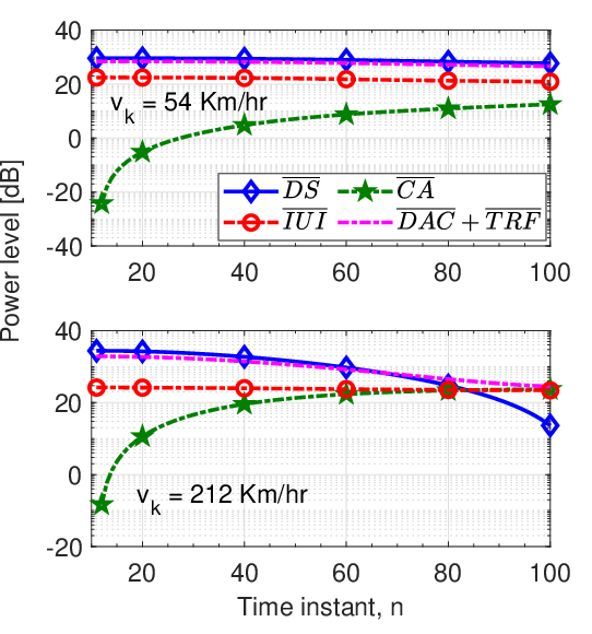
Refer to caption
(a)
Refer to caption
(b)
Refer to caption
(c)
Refer to caption
(d)
Figure 4: a) Comparison of LSFD and SLD for different UE configuration; Effect of channel aging on the power of desired and interference terms for b) LSFD; and c) SLD; and d) SE versus number of antenna per AP for different UE velocities.

We next compare Fig. 4(b) with Fig. 4(c), which plots the above power values for SLD. We see that for low-velocity UEs, LSFD has a much lower IUI¯\overline{\text{IUI}}, CA¯\overline{\text{CA}} and DAC¯+TRF¯\overline{\text{DAC}}+\overline{\text{TRF}} power than SLD. This is because the channels of low-velocity UEs do not significantly age, and consequently their channel estimate quality do not deteriorate. The LSFD can thus better suppress the IUI. For high-velocity UEs, LSFD yields much lower CA¯\overline{\text{CA}} values than SLD, while both LSFD and SLD yield similar IUI¯\overline{\text{IUI}} values. This implies that LSFD can mitigate the effect of channel aging for high-velocity UEs, but not IUI. This study not only validates the interference-related insights in Corollary 3, but also shows that LSFD can mitigate i) the effect of channel aging for low/high UE velocities; and ii) IUI, but only for low-velocity UEs.

V-6 Impact of AP antennas on the UE velocity

We now investigate in Fig. 4(d) the SE versus number of antennas per AP (NN) for different UE velocities: vk={0,54,128}v_{k}=\{0,54,128\} Km/hr. We see that the SE increasing with NN. This is due to the increased array gain. We also infer that for different NN values, the %\% of SE loss for vk=54v_{k}=54 Km/hr (resp. vk=128v_{k}=128 Km/hr) over vk=0v_{k}=0 Km/hr is same i.e., 5%5\% (resp. 19%19\%). This crucially informs that the SE degradation due to channel aging is independent of the NN value, and depends only on the UE speed.

V-7 Dynamic ADC architecture across APs/antennas

To investigate the effect of dynamic ADC architecture, we plot in Fig. 5(a) the SE versus transmit power and compare for the following ADC architectures: i) ideal ADCs; ii) Dynamic ADC - antennas: 25%25\% of the antennas at each AP has 11, 22, 33 and 44 bit ADC resolutions; and iii) Dynamic ADC - APs: 25%25\% of the APs have 11, 22, 33 and 44 bit resolution. We see from Fig. 5(a) that Dynamic ADC −- antennas architecture yields a similar SE as that of Dynamic ADC −- APs architecture. Also, both dynamic architectures provide nearly 84%84\% of the ideal ADCs SE. For this study, we assume that each AP has 44 antennas.

This shows the flexibility of dynamic ADC architecture, which allows the system designer to either have different ADC resolution across the antennas of each AP or across APs.

V-8 SE versus UE transmit power

We now plot in Fig. 5(b), the SE obtained using the proposed optimization algorithms: CVX-based (labelled as MM) and Algorithm 1 (labelled as closed-form MM) for LSFD and SLD schemes. We also compare them with full power allocation (FPA) scheme, where each UE transmits at its maximum power. We fix M=64M=64 APs, K=20K=20 UEs, N=4N=4 antennas, κ=0.1\kappa=0.1 and b=4b=4 bits at both APs and UEs. We first see that both CVX-based and closed-form MM provide a similar SE, but the latter with its closed-form transmit power updates, has a trivial complexity. It can, therefore, be easily implemented in commercial CF systems. Also, both proposed optimizations improve the SE by 20%20\% in SLD, whereas they provide a reduced gain of 6.25%6.25\% in LSFD. This is because SLD is unable to effectively mitigate the IUI, which in turn is mitigated by using the optimal powers designed by the proposed algorithms. The LSFD, in contrast, mitigates the IUI by performing an extra level of decoding at the CPU, and optimizing transmit power, therefore, only provides marginal SE gain.

Refer to caption
(a)
Refer to caption
(b)
Refer to caption
(c)
Refer to caption
(d)
Figure 5: a) Comparison of different ADC architectures; b) SE versus UE transmit power; c) SE versus time instant nn; d) CPU and average run time for different optimization techniques.

V-9 Effect of channel aging on SE optimization

We now study in Fig. 5(c), the effect of optimization time instant on the sum SE for the following UE velocities vk={54,212}v_{k}=\{54,212\} Km/hr. We optimize the SE at a specific time-instant, denoted as noptn_{\text{opt}}, and use the obtained optimal transmit powers to calculate the SE for all time-instants. We compare in Fig. 5(c), the SE for:

  • •

    Case 1: SE is optimized at every data transmission instant i.e., nopt=nn_{\text{opt}}=n.

  • •

    Case 2: SE is optimized at one of the following time instants nopt={τp+1,τc4,τc2,3​τc4}n_{\text{opt}}=\{\tau_{p}+1,\frac{\tau_{c}}{4},\frac{\tau_{c}}{2},\frac{3\tau_{c}}{4}\}.

We perform this study for two different UE velocities of vk=54v_{k}=54 Km/hr and vk=212v_{k}=212 Km/hr. We see that for a low UE velocity of vk=54v_{k}=54 Km/hr, Case 2, irrespective of the optimizing time-instant noptn_{\text{opt}} yields a similar SE as that of Case 1 for all time instants. For a high UE velocity of vk=212v_{k}=212 Km/hr, Case 1 and Case 2 with nopt≤3​τc4n_{\text{opt}}\leq\frac{3\tau_{c}}{4} has similar SE. But, for nopt=τcn_{\text{opt}}=\tau_{c}, Case 2 yields only a minor 10%10\% lower SE than Case 1, and that too during initial time instants. The SE thus can be optimized in the beginning of the resource block and its solution could be reported only once, which makes the proposed optimization practical.

V-10 Optimization complexity

We now analyze the time complexity of both the proposed iterative optimization MM techniques – CVX-based and closed-form – by first plotting in Fig. 5(d) their total CPU run time required to converge. We see that the later approach requires much lesser time to converge. Also, both the techniques converge to the same SE value. We next also investigate the average per-iteration CPU run time required by both algorithms (shown in the sub-plot). We see that the closed-form technique has a much lesser run-time per iteration. This is due to its closed-form power updates with trivial complexity.

VI Conclusion

We derived a closed-form SE expression for a hardware-impaired spatially-correlated Rician-faded CF mMIMO system with channel aging and two-layer LSFD. We verified this expression for different transmit power and hardware impairment values. We optimized the non-convex SE metric by proposing two novel optimization techniques. The first one has a high complexity, while the second provides a closed-form solution with a trivial complexity. We numerically showed that the two-layer LSFD effectively mitigates the interference due to channel aging for both low- and high-velocity UEs. It, however, mitigates inter-user interference only for the low-velocity UEs, and not the fast ones. We also showed that the SE loss due to hardware impairments can be compensated by the proposed dynamic ADC architecture.

Appendix A

The LMMSE estimate of the channel 𝐡m​k\mathbf{h}_{mk}, based on received pilot signal in (7) is given by

𝐡^m​k​[λ]=𝐂𝐡m​k​[λ]​𝐲m​[tk]​𝐂𝐲m​[tk]​𝐲m​[tk]−1​𝐲m​[tk].\displaystyle\hat{\mathbf{h}}_{mk}[\lambda]=\mathbf{C}_{\mathbf{h}_{mk}[\lambda]\mathbf{y}_{m}[t_{k}]}\mathbf{C}_{\mathbf{y}_{m}[t_{k}]\mathbf{y}_{m}[t_{k}]}^{-1}\mathbf{y}_{m}[t_{k}]. (34)

Here 𝐂𝐡m​k​[λ]​𝐲mp​[tk]=𝔼⁡{𝐡m​k​[λ]​(𝐲ADC,mp​[tk])H}\mathbf{C}_{\mathbf{h}_{mk}[\lambda]\mathbf{y}_{m}^{p}[t_{k}]}=\mathbb{E}\big\{\mathbf{h}_{mk}[\lambda](\mathbf{y}^{p}_{\text{ADC},m}[t_{k}])^{H}\big\} and 𝐂𝐲mp​[tk]​𝐲mp​[tk]=𝔼⁡{𝐲ADC,mp​[tk]​(𝐲ADC,mp​[tk])H}\mathbf{C}_{\mathbf{y}_{m}^{p}[t_{k}]\mathbf{y}^{p}_{m}[t_{k}]}=\mathbb{E}\big\{\mathbf{y}_{\text{ADC},m}^{p}[t_{k}](\mathbf{y}^{p}_{\text{ADC},m}[t_{k}])^{H}\big\}.

We begin by simplifying the term 𝐂𝐲m​[tk]​𝐲m​[tk]\mathbf{C}_{\mathbf{y}_{m}[t_{k}]\mathbf{y}_{m}[t_{k}]} by substituting 𝐲ADC,m​[tk]\mathbf{y}_{\text{ADC},m}[t_{k}] from (7) as

𝐂𝐲m​[tk]​𝐲m​[tk]\displaystyle\mathbf{C}_{\mathbf{y}_{m}[t_{k}]\mathbf{y}_{m}[t_{k}]} =(a)​∑j∈𝒫k𝐀m​αd,j2​p~j​𝐑¯m​j​𝐀mH+∑j∈𝒫k𝐀m​(1−αd,j+κt,j2)​αd,j​p~j​𝐑¯m​j​𝐀mH\displaystyle\overset{(a)}{=}\sum_{j\in\mathcal{P}_{k}}\mathbf{A}_{m}\alpha_{d,j}^{2}\tilde{p}_{j}\bar{\mathbf{R}}_{mj}\mathbf{A}_{m}^{H}+\sum_{j\in\mathcal{P}_{k}}\mathbf{A}_{m}(1-\alpha_{d,j}+\kappa_{t,j}^{2})\alpha_{d,j}\tilde{p}_{j}\bar{\mathbf{R}}_{mj}\mathbf{A}_{m}^{H}
+κr,m2​𝐉k+𝐁m​((1+κr,m2)​𝐉​[tk]+σ2​𝐈N)+σ2​𝐀m​𝐀mH\displaystyle\qquad+\kappa^{2}_{r,m}\mathbf{J}_{k}+\mathbf{B}_{m}\big((1+\kappa_{r,m}^{2})\mathbf{J}[t_{k}]+\sigma^{2}\mathbf{I}_{N}\big)+\sigma^{2}\mathbf{A}_{m}\mathbf{A}_{m}^{H}
=∑j∈𝒫k𝐀m​αd,j​(1+κt,j2)​p~j​𝐑¯m​j​𝐀mH+(𝐁am+κr,m2​𝐀m)​𝐉+σ2​𝐀m.\displaystyle=\sum_{j\in\mathcal{P}_{k}}\mathbf{A}_{m}\alpha_{d,j}(1+\kappa_{t,j}^{2})\tilde{p}_{j}\mathbf{\overline{R}}_{mj}\mathbf{A}_{m}^{H}+\big(\mathbf{B}_{a}^{m}+\kappa^{2}_{r,m}\mathbf{A}_{m}\big)\mathbf{J}+\sigma^{2}\mathbf{A}_{m}. (35)

Here 𝐉k=∑j∈𝒫k(1+κt,j2)​αd,j​p~j​diag​(𝐑¯m​j)\mathbf{J}_{k}=\sum_{j\in\mathcal{P}_{k}}(1+\kappa_{t,j}^{2})\alpha_{d,j}\tilde{p}_{j}\text{diag}\big(\bar{\mathbf{R}}_{mj}\big). Equality (a)(a) is obtained by noting that the i) distortion terms υDAC,kp​[tk],ξRF,kp​[tk],𝜼RF,mp​[tk]\upsilon_{\text{DAC},k}^{p}[t_{k}],\xi_{\text{RF},k}^{p}[t_{k}],\boldsymbol{\eta}^{p}_{\text{RF},m}[t_{k}] and 𝐧ADC,mp​[tk]\mathbf{n}_{\text{ADC},m}^{p}[t_{k}] are independent of each other, and have a zero mean; and ii) variance of distortion/quantization noises are 𝔼⁡{ξRF,jp​[tk]​(ξRF,jp​[tk])H}=κt,j2​αd,j​p~j\mathbb{E}\{\xi_{\text{RF},j}^{p}[t_{k}](\xi^{p}_{\text{RF},j}[t_{k}])^{H}\}\!=\kappa_{t,j}^{2}\alpha_{d,j}\tilde{p}_{j}, 𝔼⁡{𝐧ADC,mp​[tk]​(𝐧ADC,mp​[tk])H}=𝐁m​𝐒m​[tk]\mathbb{E}\{\mathbf{n}_{\text{ADC},m}^{p}[t_{k}](\mathbf{n}_{\text{ADC},m}^{p}[t_{k}])^{H}\}=\mathbf{B}_{m}\mathbf{S}^{m}[t_{k}], 𝔼⁡{𝜼RF,mp​[tk]​(𝜼RF,mp​[tk])H}=κr,m2​𝐖m​[tk]\mathbb{E}\{\boldsymbol{\eta}_{\text{RF},m}^{p}[t_{k}](\boldsymbol{\eta}^{p}_{\text{RF},m}[t_{k}])^{H}\}=\kappa^{2}_{r,m}{\mathbf{W}}^{m}[t_{k}]; and iii) impairment/quantization noises are independent of channel 𝐡m​k\mathbf{h}_{mk}. Here the matrices 𝐖m​[tk]=∑j∈𝒫k(1+κt,j2)​αd,j​p~j​diag​(𝐡m​j​[tk]​𝐡m​jH​[tk])\mathbf{W}^{m}[t_{k}]=\sum_{j\in\mathcal{P}_{k}}(1+\kappa_{t,j}^{2})\alpha_{d,j}\tilde{p}_{j}\text{diag}\big(\mathbf{h}_{mj}[t_{k}]\mathbf{h}_{mj}^{H}[t_{k}]\big) and 𝐒m​[n]=(1+κr,m2)​𝐖m​[tk]+σ2​𝐈N\mathbf{S}^{m}[n]=(1+\kappa_{r,m}^{2})\mathbf{W}^{m}[t_{k}]+\sigma^{2}\mathbf{I}_{N}. We, similarly, have 𝐂𝐡m​k​[λ]​𝐲mp​[tk]\mathbf{C}_{\mathbf{h}_{mk}[\lambda]\mathbf{y}_{m}^{p}[t_{k}]} as 𝐂𝐡m​k​[λ]​𝐲mp​[tk]=αd,k​p~k​ρk​[λ−tk]​𝐑¯m​k​𝐀m\mathbf{C}_{\mathbf{h}_{mk}[\lambda]\mathbf{y}_{m}^{p}[t_{k}]}=\alpha_{d,k}\sqrt{\tilde{p}_{k}}\rho_{k}[\lambda\!-\!t_{k}]\bar{\mathbf{R}}_{mk}\mathbf{A}_{m}.

Appendix B

To obtain the result (a) in Table III, we first express 𝐡m​i​[tk]\mathbf{h}_{mi}[t_{k}] and 𝐡m​i​[n]\mathbf{h}_{mi}[n] in terms of 𝐡m​i​[λ]\mathbf{h}_{mi}[\lambda], 𝐮m​i​[tk]\mathbf{u}_{mi}[t_{k}] and 𝐮m​i​[n]\mathbf{u}_{mi}[n] as

𝔼⁡{𝐡m​iH​[tk]​𝐀am​𝐏m​k​diag​(𝐡m​i​[n]​𝐡m​iH​[n])​𝐏m​kH​𝐀am​𝐡m​i​[tk]}\displaystyle\mathbb{E}\left\{\mathbf{h}_{mi}^{H}[t_{k}]\mathbf{A}_{a}^{m}\mathbf{P}_{mk}\text{diag}(\mathbf{h}_{mi}[n]\mathbf{h}_{mi}^{H}[n])\mathbf{P}_{mk}^{H}\mathbf{A}_{a}^{m}\mathbf{h}_{mi}[t_{k}]\right\}
=ρi2​[λ−tk]​𝔼​{𝐡m​iH​[λ]​𝐀am​𝐏m​k​diag​(ρi2​[n−λ]​𝐡m​i​[λ]​𝐡m​iH​[λ])​𝐏m​kH​𝐀am​𝐡m​i​[λ]}\displaystyle\quad\qquad=\rho_{i}^{2}[\lambda-t_{k}]\mathbb{E}\big\{\mathbf{h}_{mi}^{H}[\lambda]\mathbf{A}_{a}^{m}\mathbf{P}_{mk}\text{diag}(\rho_{i}^{2}[n-\lambda]\mathbf{h}_{mi}[\lambda]\mathbf{h}_{mi}^{H}[\lambda])\mathbf{P}_{mk}^{H}\mathbf{A}_{a}^{m}\mathbf{h}_{mi}[\lambda]\big\}
+(ρi2​[λ−tk]​ρ¯i2​[n−λ]+ρ¯i2​[λ−tk])​tr​(𝐑¯m​i​𝐀am​𝐏m​k​diag​(𝐑¯m​i)​𝐏m​kH​𝐀am).\displaystyle\qquad\qquad+\big(\rho_{i}^{2}[\lambda-t_{k}]\bar{\rho}_{i}^{2}[n-\lambda]+\bar{\rho}_{i}^{2}[\lambda-t_{k}]\big)\text{tr}\left(\bar{\mathbf{R}}_{mi}\mathbf{A}_{a}^{m}\mathbf{P}_{mk}\text{diag}\big(\bar{\mathbf{R}}_{mi}\big)\mathbf{P}_{mk}^{H}\mathbf{A}_{a}^{m}\right). (36)

Equality (a)(a) is obtained by substituting 𝔼⁡{𝐮m​i​[tk]​𝐮m​iH​[tk]}=𝔼⁡{𝐮m​i​[n]​𝐮m​iH​[n]}=𝐑m​i\mathbb{E}\{\mathbf{u}_{mi}[t_{k}]\mathbf{u}^{H}_{mi}[t_{k}]\}\!=\!\mathbb{E}\{\mathbf{u}_{mi}[n]\mathbf{u}^{H}_{mi}[n]\}\!=\!\mathbf{R}_{mi} as [40]. We now calculate the expectation in the first term of (36) by substituting the value of 𝐡m​i​[λ]\mathbf{h}_{mi}[\lambda] as

𝔼⁡{𝐡m​iH​[λ]​𝐀am​𝐏m​k​diag​(𝐡m​i​[λ]​𝐡m​iH​[λ])​𝐏m​kH​𝐀am​𝐡m​i​[λ]}\displaystyle\mathbb{E}\big\{\mathbf{h}_{mi}^{H}[\lambda]\mathbf{A}_{a}^{m}\mathbf{P}_{mk}\text{diag}(\mathbf{h}_{mi}[\lambda]\mathbf{h}_{mi}^{H}[\lambda])\mathbf{P}_{mk}^{H}\mathbf{A}_{a}^{m}\mathbf{h}_{mi}[\lambda]\big\}
=𝐡¯m​iH​𝐀am​𝐏m​k​diag​(𝐡¯m​i​𝐡¯m​iH+𝐑m​i)​𝐏m​kH​𝐀am​𝐡¯m​i+Tr​(𝐑m​i​𝐀am​𝐏m​k​diag​(𝐡¯m​i​𝐡¯m​iH)​𝐏m​kH​𝐀am)\displaystyle=\bar{\mathbf{h}}_{mi}^{H}\mathbf{A}_{a}^{m}\mathbf{P}_{mk}\text{diag}(\bar{\mathbf{h}}_{mi}\bar{\mathbf{h}}_{mi}^{H}+\mathbf{R}_{mi})\mathbf{P}_{mk}^{H}\mathbf{A}_{a}^{m}\bar{\mathbf{h}}_{mi}+\text{Tr}\left(\mathbf{R}_{mi}\mathbf{A}_{a}^{m}\mathbf{P}_{mk}\text{diag}(\bar{\mathbf{h}}_{mi}\bar{\mathbf{h}}_{mi}^{H})\mathbf{P}_{mk}^{H}\mathbf{A}_{a}^{m}\right)
+2​real​{𝔼⁡{𝐡¯m​iH​𝐀am​𝐏m​k​d​i​a​g​(𝐡¯m​i​𝐡~m​iH​[λ]​𝐑m​i1/2)​𝐏m​kH​𝐀am​𝐑m​i1/2​𝐡~m​i​[λ]}}\displaystyle\quad+2\text{real}\Big\{\mathbb{E}\big\{\bar{\mathbf{h}}_{mi}^{H}\mathbf{A}_{a}^{m}\mathbf{P}_{mk}diag(\bar{\mathbf{h}}_{mi}{\tilde{\mathbf{h}}}_{mi}^{H}[\lambda]\mathbf{R}_{mi}^{1/2})\mathbf{P}_{mk}^{H}\mathbf{A}_{a}^{m}\mathbf{R}_{mi}^{1/2}{\tilde{\mathbf{h}}}_{mi}[\lambda]\big\}\Big\}
+𝔼⁡{𝐡~m​iH​[λ]​𝐑m​i1/2​𝐀am​𝐏m​k​d​i​a​g​(𝐑m​i1/2​𝐡~m​i​[λ]​𝐡~m​iH​[λ]​𝐑m​i1/2)​𝐏m​kH​𝐀am​𝐑m​i1/2​𝐡~m​i​[λ]}\displaystyle\quad+\mathbb{E}\Big\{{\tilde{\mathbf{h}}}_{mi}^{H}[\lambda]\mathbf{R}_{mi}^{1/2}\mathbf{A}_{a}^{m}\mathbf{P}_{mk}diag(\mathbf{R}_{mi}^{1/2}{\tilde{\mathbf{h}}}_{mi}[\lambda]{\tilde{\mathbf{h}}}_{mi}^{H}[\lambda]\mathbf{R}_{mi}^{1/2})\mathbf{P}_{mk}^{H}\mathbf{A}_{a}^{m}\mathbf{R}_{mi}^{1/2}{\tilde{\mathbf{h}}}_{mi}[\lambda]\Big\}
=𝐡¯m​iH​𝐀am​𝐏m​k​diag​(𝐡¯m​i​𝐡¯m​iH+𝐑m​i)​𝐏m​kH​𝐀am​𝐡¯m​i+Tr​(𝐑m​i​𝐀am​𝐏m​k​diag​(𝐡¯m​i​𝐡¯m​iH)​𝐏m​kH​𝐀am)\displaystyle=\bar{\mathbf{h}}_{mi}^{H}\mathbf{A}_{a}^{m}\mathbf{P}_{mk}\text{diag}(\bar{\mathbf{h}}_{mi}\bar{\mathbf{h}}_{mi}^{H}+\mathbf{R}_{mi})\mathbf{P}_{mk}^{H}\mathbf{A}_{a}^{m}\bar{\mathbf{h}}_{mi}+\text{Tr}\left(\mathbf{R}_{mi}\mathbf{A}_{a}^{m}\mathbf{P}_{mk}\text{diag}(\bar{\mathbf{h}}_{mi}\bar{\mathbf{h}}_{mi}^{H})\mathbf{P}_{mk}^{H}\mathbf{A}_{a}^{m}\right)
+2​real​{𝔼⁡{∑j(∑n1[𝐡¯m​i]n1∗​[𝐡¯m​i]j​[𝐀m​𝐏m​k]n1​j)​(∑n2[𝐏m​kH​𝐀m]j​n2​[𝐡~m​iH​[λ]​𝐑m​i1/2]j​[𝐑m​i1/2​𝐡~m​i​[λ]]n2)}}\displaystyle+\!2\text{real}\Big\{\mathbb{E}\Big\{\!\sum_{j}\Big(\!\sum_{n_{1}}[\bar{\mathbf{h}}_{mi}]_{n_{1}}^{*}[\bar{\mathbf{h}}_{mi}]_{j}[\mathbf{A}_{m}\mathbf{P}_{\!mk}]_{n_{1}j}\!\Big)\Big(\!\sum_{n_{2}}[\mathbf{P}_{\!mk}^{H}\mathbf{A}_{m}]_{jn_{2}}[{\tilde{\mathbf{h}}}_{mi}^{H}[\lambda]\mathbf{R}_{mi}^{1/2}]_{j}[\mathbf{R}_{mi}^{1/2}\tilde{\mathbf{h}}_{mi}[\lambda]]_{n_{2}}\!\Big)\!\Big\}\Big\}
+(∑j∑n1∑n2∑n3∑n4𝔼⁡{[𝐡~m​i∗​[λ]]n1​[𝐡~m​i​[λ]]n​2​[𝐡~m​i∗​[λ]]n​3​[𝐡~m​i​[λ]]n​4}CLOSE\displaystyle+\Big(\sum_{j}\sum_{n_{1}}\sum_{n_{2}}\sum_{n_{3}}\sum_{n_{4}}\mathbb{E}\Big\{[{\tilde{\mathbf{h}}}_{mi}^{*}[\lambda]]_{n_{1}}[{\tilde{\mathbf{h}}}_{mi}[\lambda]]_{n2}[{\tilde{\mathbf{h}}}_{mi}^{*}[\lambda]]_{n3}[{\tilde{\mathbf{h}}}_{mi}[\lambda]]_{n4}\Big\}
×[𝐑m​i1/2𝐀am𝐏m​k]n1​j[𝐑m​i1/2]j​n2[𝐑m​i1/2]n3​j[𝐏m​kH𝐀am𝐑m​i1/2]j​n4).\displaystyle\qquad\times[\mathbf{R}_{mi}^{1/2}\mathbf{A}_{a}^{m}\mathbf{P}_{mk}]_{n_{1}j}[\mathbf{R}_{mi}^{1/2}]_{jn_{2}}[\mathbf{R}_{mi}^{1/2}]_{n_{3}j}[\mathbf{P}_{mk}^{H}\mathbf{A}_{a}^{m}\mathbf{R}_{mi}^{1/2}]_{jn_{4}}\Big). (37)

Here, the terms [𝐡¯m​i]n1[\bar{\mathbf{h}}_{mi}]_{n_{1}} and [𝐡~m​i∗​[λ]]n1[{\tilde{\mathbf{h}}}_{mi}^{*}[\lambda]]_{n_{1}} represent the n1n_{1}th element of the vectors 𝐡¯m​i\bar{\mathbf{h}}_{mi} and 𝐡~m​i∗​[λ]{\tilde{\mathbf{h}}}_{mi}^{*}[\lambda], respectively. The terms [𝐀am​𝐏m​k]n1​j[\mathbf{A}_{a}^{m}\mathbf{P}_{mk}]_{n_{1}j} and [𝐑m​i1/2​𝐀am​𝐏m​k]n1​j[\mathbf{R}_{mi}^{1/2}\mathbf{A}_{a}^{m}\mathbf{P}_{mk}]_{n_{1}j} represent the (n1,j)(n_{1},j)th element of the matrices 𝐀am​𝐏m​k\mathbf{A}_{a}^{m}\mathbf{P}_{mk} and 𝐑m​i1/2​𝐀am​𝐏m​k\mathbf{R}_{mi}^{1/2}\mathbf{A}_{a}^{m}\mathbf{P}_{mk}, respectively. We note that, in the last term, the expectation 𝔼⁡{[𝐡~m​i∗​[λ]]n1​[𝐡~m​i​[λ]]n2​[𝐡~m​i∗​[λ]]n​3​[𝐡~m​i​[λ]]n​4}\mathbb{E}\big\{[{\tilde{\mathbf{h}}}_{mi}^{*}[\lambda]]_{n_{1}}[{\tilde{\mathbf{h}}}_{mi}[\lambda]]_{n_{2}}[{\tilde{\mathbf{h}}}_{mi}^{*}[\lambda]]_{n3}[{\tilde{\mathbf{h}}}_{mi}[\lambda]]_{n4}\big\} is non-zero only when either n1=n2=m1;n3=n4=m2n_{1}\!=\!n_{2}\!=\!m_{1};n_{3}\!=\!n_{4}\!=\!m_{2} or n1=n4=m1;n2=n3=m2n_{1}\!=\!n_{4}\!=\!m_{1};n_{2}\!=n_{3}\!=m_{2}. We can, therefore, calculate the expectations in (37) as

𝔼⁡{𝐡m​iH​[λ]​𝐀m​𝐏m​k​diag​(𝐡m​i​[λ]​𝐡m​iH​[λ])​𝐏m​kH​𝐀m​𝐡m​i​[λ]}\displaystyle\!\!\!\!\mathbb{E}\Big\{\mathbf{h}_{mi}^{H}[\lambda]\mathbf{A}_{m}\mathbf{P}_{mk}\text{diag}(\mathbf{h}_{mi}[\lambda]\mathbf{h}_{mi}^{H}[\lambda])\mathbf{P}_{mk}^{H}\mathbf{A}_{m}\mathbf{h}_{mi}[\lambda]\Big\}
=𝐡¯m​iH​𝐀m​𝐏m​k​diag​(𝐡¯m​i​𝐡¯m​iH+𝐑m​i)​𝐏m​kH​𝐀am​𝐡¯m​i+Tr​(𝐑m​i​𝐀m​𝐏m​k​diag​(𝐡¯m​i​𝐡¯m​iH)​𝐏m​kH​𝐀m)\displaystyle\!\!\!\!\!=\bar{\mathbf{h}}_{mi}^{H}\mathbf{A}_{m}\mathbf{P}_{mk}\text{diag}(\bar{\mathbf{h}}_{mi}\bar{\mathbf{h}}_{mi}^{H}+\mathbf{R}_{mi})\mathbf{P}_{mk}^{H}\mathbf{A}_{a}^{m}\bar{\mathbf{h}}_{mi}+\text{Tr}\left(\mathbf{R}_{mi}\mathbf{A}_{m}\mathbf{P}_{mk}\text{diag}(\bar{\mathbf{h}}_{mi}\bar{\mathbf{h}}_{mi}^{H})\mathbf{P}_{mk}^{H}\mathbf{A}_{m}\right)
+2​real​{∑j(∑n1[𝐡¯m​i​𝐡¯m​iH]j​n1​[𝐀m​𝐏m​k]n1​j)​(∑n2[𝐏m​kH​𝐀m]j​n2​[𝐑m​i]n2​j)}\displaystyle\!\!\!\!\!\quad+2\text{real}\Big\{\sum_{j}\Big(\sum_{n_{1}}[\bar{\mathbf{h}}_{mi}\bar{\mathbf{h}}_{mi}^{H}]_{jn_{1}}[\mathbf{A}_{m}\mathbf{P}_{mk}]_{n_{1}j}\Big)\Big(\sum_{n_{2}}[\mathbf{P}_{mk}^{H}\mathbf{A}_{m}]_{jn_{2}}[\mathbf{R}_{mi}]_{n_{2}j}\Big)\Big\}
+∑j∑m1∑m2[𝐑m​i1/2𝐀m𝐏m​k]m1​j[𝐑m​i1/2]j​m1[𝐑m​i1/2]m2​j[𝐏m​kH𝐀m𝐑m​i1/2]j​m2\displaystyle\!\!\!\!\!\quad+\sum_{j}\sum_{m_{1}}\sum_{m_{2}}[\mathbf{R}_{mi}^{1/2}\mathbf{A}_{m}\mathbf{P}_{mk}]_{m_{1}j}[\mathbf{R}_{mi}^{1/2}]_{jm_{1}}[\mathbf{R}_{mi}^{1/2}]_{m_{2}j}[\mathbf{P}_{mk}^{H}\mathbf{A}_{m}\mathbf{R}_{mi}^{1/2}]_{jm_{2}}
+∑j∑m1∑m2[𝐑m​i1/2𝐀m𝐏m​k]m1​j[𝐑m​i1/2]j​m2[𝐑m​i1/2]m2​j[𝐏m​kH𝐀m𝐑m​i1/2]j​m1\displaystyle\quad+\sum_{j}\sum_{m_{1}}\sum_{m_{2}}[\mathbf{R}_{mi}^{1/2}\mathbf{A}_{m}\mathbf{P}_{mk}]_{m_{1}j}[\mathbf{R}_{mi}^{1/2}]_{jm_{2}}[\mathbf{R}_{mi}^{1/2}]_{m_{2}j}[\mathbf{P}_{mk}^{H}\mathbf{A}_{m}\mathbf{R}_{mi}^{1/2}]_{jm_{1}} (38)
=(d)​Tr​((𝐡¯m​i​𝐡¯m​iH+𝐑m​i)​𝐀m​𝐏m​k​diag​(𝐡¯m​i​𝐡¯m​iH+𝐑m​i)​𝐏m​kH​𝐀am)\displaystyle\!\!\!\!\!\overset{(d)}{=}\text{Tr}\!\left(\left(\bar{\mathbf{h}}_{mi}\bar{\mathbf{h}}_{mi}^{H}+\mathbf{R}_{mi}\right)\mathbf{A}_{m}\mathbf{P}_{mk}\text{diag}\left(\bar{\mathbf{h}}_{mi}\bar{\mathbf{h}}_{mi}^{H}+\mathbf{R}_{mi}\right)\mathbf{P}_{mk}^{H}\mathbf{A}_{a}^{m}\right)
+2​real​{Tr​(𝐡¯m​i​𝐡¯m​iH​𝐀m​𝐏m​k​diag​(𝐏m​kH​𝐀m​𝐑m​i))}+Tr​(𝐑m​i​𝐀m​𝐏m​k​diag​(𝐏m​kH​𝐀m​𝐑m​i)).\displaystyle\!\!\!\!\!\quad+2\text{real}\left\{\text{Tr}\!\left(\bar{\mathbf{h}}_{mi}\bar{\mathbf{h}}_{mi}^{H}\mathbf{A}_{m}\mathbf{P}_{\!mk}\text{diag}\!\left(\mathbf{P}_{\!mk}^{H}\mathbf{A}_{m}\mathbf{R}_{mi}\right)\right)\right\}\!+\!\text{Tr}\!\left(\mathbf{R}_{mi}\mathbf{A}_{m}\mathbf{P}_{\!mk}\text{diag}\!\left(\mathbf{P}_{\!mk}^{H}\mathbf{A}_{m}\mathbf{R}_{mi}\right)\right). (39)

Equality (d)(d) is obtained by expressing the summation terms in matrix form and using algebraic operations. Substituting (39) in (36), we obtain first result in Table III. Similarly, we can simplify the term 𝔼⁡{𝐡m​iH​[λ]​𝐀m​𝐏m​k​𝐡m​i​[λ]​𝐡m​iH​[λ]​𝐏m​kH​𝐀m​𝐡m​i​[λ]}\mathbb{E}\{\mathbf{h}_{mi}^{H}[\lambda]\mathbf{A}_{m}\mathbf{P}_{mk}\mathbf{h}_{mi}[\lambda]\mathbf{h}_{mi}^{H}[\lambda]\mathbf{P}_{mk}^{H}\mathbf{A}_{m}\mathbf{h}_{mi}[\lambda]\} to obtain the second result in Table III.

Appendix C

We now derive Theorem 2 by computing the following expectations.
Computation of DS¯k,n\overline{\text{DS}}_{k,n}: The power of the desired signal can be calculated as

DS¯k,n=|∑m=1M𝐚m​k∗​[n]​ρ​[n−λ]​(αd,k)​pk​𝔼​{𝐡^m​kH​[λ]​𝐀m​𝐡m​k​[λ]}|2.\displaystyle\overline{\text{DS}}_{k,n}=\Big|\sum_{m=1}^{M}\mathbf{a}_{mk}^{*}[n]\rho[n-\lambda]\left(\alpha_{d,k}\right)\sqrt{p_{k}}\mathbb{E}\left\{\hat{\mathbf{h}}_{mk}^{H}[\lambda]\mathbf{A}_{m}\mathbf{h}_{mk}[\lambda]\right\}\Big|^{2}. (40)

We now compute 𝔼⁡{𝐡^m​kH​[λ]​𝐀m​𝐡m​k​[λ]}\mathbb{E}\big\{\hat{\mathbf{h}}_{mk}^{H}[\lambda]\mathbf{A}_{m}\mathbf{h}_{mk}[\lambda]\big\} by substituting 𝐡^m​k\hat{\mathbf{h}}_{mk} using (8) as

𝔼⁡{𝐡^m​kH​[λ]​𝐀m​𝐡m​k​[λ]}=αd,k​p~k​ρk​[λ−tk]​tr​(𝐀m​𝔼​{𝐡m​k​[λ]​𝐲ADC,mH​[tk]}​𝚿m​k​𝐀m​𝐑¯m​k)\displaystyle\mathbb{E}\left\{\hat{\mathbf{h}}_{mk}^{H}[\lambda]\mathbf{A}_{m}\mathbf{h}_{mk}[\lambda]\right\}=\alpha_{d,k}\sqrt{\tilde{p}_{k}}\rho_{k}[\lambda-t_{k}]\text{tr}\left(\mathbf{A}_{m}\mathbb{E}\left\{\mathbf{h}_{mk}[\lambda]\mathbf{y}_{\text{ADC},m}^{H}[t_{k}]\right\}\boldsymbol{\Psi}_{mk}\mathbf{A}_{m}\bar{\mathbf{R}}_{mk}\right)
=αd,k2​p~k​ρk2​[λ−tk]​tr​(𝐀m​𝐑¯m​k​𝐀m​𝚿m​k​𝐀m​𝐑¯m​k)=tr​(𝐀m​𝚪¯m​k).\displaystyle\qquad=\alpha_{d,k}^{2}\tilde{p}_{k}\rho_{k}^{2}[\lambda-t_{k}]\text{tr}\left(\mathbf{A}_{m}\bar{\mathbf{R}}_{mk}\mathbf{A}_{m}\boldsymbol{\Psi}_{mk}\mathbf{A}_{m}\bar{\mathbf{R}}_{mk}\right)=\text{tr}\left(\mathbf{A}_{m}\boldsymbol{\overline{\Gamma}}_{mk}\right). (41)

Substituting (41) in (40), we get DS¯k,n=|∑m=1M𝐚m​k∗​[n]​ρ​[n−λ]​αd,k​pk​tr​(𝐀m​𝚪¯m​k)|2\overline{\text{DS}}_{k,n}\!=\!\big|\sum_{m=1}^{M}\!\mathbf{a}_{mk}^{*}[n]\rho[n\!-\!\lambda]\alpha_{d,k}\!\sqrt{p_{k}}\text{tr}\left(\mathbf{A}_{m}\boldsymbol{\overline{\Gamma}}_{mk}\right)\big|^{2}.
Computation of IUI¯k​i,n\overline{{\mbox{IUI}}}_{ki,n}: The power of inter-user interference can be computed as

IUI¯k​i,n\displaystyle\overline{{\mbox{IUI}}}_{ki,n}\! =𝔼⁡{|∑m=1Mam​k∗​[n]​αd,i​pi​𝐡^m​kH​[λ]​𝐀m​𝐡m​i​[n]|2}=αd,i2​pi​∑m=1M(|am​k∗​[n]|2​𝔼⁡{|𝐡^m​kH​[λ]​𝐀m​𝐡m​i​[n]|2}⏟ck​i​n,mCLOSE\displaystyle=\!\mathbb{E}\bigg\{\!\Big|\sum\limits_{m=1}^{M}\!a_{mk}^{*}[n]\alpha_{d,i}\sqrt{p_{i}}\hat{\mathbf{h}}_{mk}^{H}[\lambda]\mathbf{A}_{m}\mathbf{h}_{mi}[n]\Big|^{2}\bigg\}\!=\!\alpha_{d,i}^{2}p_{i}\sum\limits_{m=1}^{M}\!\Big(|a_{mk}^{*}[n]|^{2}\underbrace{\mathbb{E}\Big\{\big|\hat{\mathbf{h}}_{mk}^{H}[\lambda]\mathbf{A}_{m}\mathbf{h}_{mi}[n]\big|^{2}\Big\}}_{c_{kin,m}}
+∑m′=1Mam​k∗[n]am′k∗[n]𝔼{𝐡^m​kH[λ]𝐀m𝐡m​i[n]𝐡^m′kH[λ]𝐀m′𝐡m′i[n]}⏟ckin,mm′).\displaystyle\quad+\sum\limits_{m^{{}^{\prime}}=1}^{M}a_{mk}^{*}[n]a_{m^{{}^{\prime}}k}^{*}[n]\underbrace{\mathbb{E}\Big\{\hat{\mathbf{h}}_{mk}^{H}[\lambda]\mathbf{A}_{m}\mathbf{h}_{mi}[n]\hat{\mathbf{h}}_{m^{{}^{\prime}}k}^{H}[\lambda]\mathbf{A}_{m^{{}^{\prime}}}\mathbf{h}_{m^{{}^{\prime}}i}[n]\Big\}}_{c_{kin,mm^{{}^{\prime}}}}\Big). (42)

We first compute the term ck​i​n,m=𝔼⁡{|𝐡^m​kH​[λ]​𝐀m​𝐡m​i​[n]|2}c_{kin,m}=\mathbb{E}\Big\{\Big|\hat{\mathbf{h}}_{mk}^{H}[\lambda]\mathbf{A}_{m}\mathbf{h}_{mi}[n]\Big|^{2}\Big\} for i∈𝒫ki\in\mathcal{P}_{k} as

ck​i​n,m∈=ρi2​[n−λ]​𝔼⁡{|𝐡^m​kH​[λ]​𝐀m​𝐡m​i​[λ]|2}⏟γ1+ρi¯2​[n−λ]​𝔼{|𝐡^m​kH[λ]𝐀m𝐮m​i′[n]|2}⏟γ2.\displaystyle c_{kin,m}^{\in}={\rho_{i}}^{2}[n-\lambda]\underbrace{\mathbb{E}\bigg\{\Big|\hat{\mathbf{h}}_{mk}^{H}[\lambda]\mathbf{A}_{m}\mathbf{h}_{mi}[\lambda]\Big|^{2}\bigg\}}_{\gamma_{1}}+\overline{\rho_{i}}^{2}[n-\lambda]\underbrace{\mathbb{E}\bigg\{\Big|\hat{\mathbf{h}}_{mk}^{H}[\lambda]\mathbf{A}_{m}\mathbf{u}_{mi}^{{}^{\prime}}[n]\Big|^{2}\bigg\}}_{\gamma_{2}}. (43)

We now compute the term γ1\gamma_{1} by first substituting 𝐡^m​k\hat{\mathbf{h}}_{mk} using (8) as

γ1\displaystyle\gamma_{1} =𝔼⁡{|𝐡^m​kH​[λ]​𝐀m​𝐡m​i​[λ]|2}=𝔼⁡{|αd,k​p~k​ρk​[λ−tk]​𝐲ADC,mH​[tk]​𝚿m​k​𝐀m​𝐑¯m​k​𝐀m​𝐡m​i​[λ]|2}\displaystyle=\mathbb{E}\Big\{\Big|\hat{\mathbf{h}}_{mk}^{H}[\lambda]\mathbf{A}_{m}\mathbf{h}_{mi}[\lambda]\Big|^{2}\Big\}=\mathbb{E}\Big\{\big|\alpha_{d,k}\sqrt{\tilde{p}_{k}}\rho_{k}[\lambda-t_{k}]\mathbf{y}_{\text{ADC},m}^{H}[t_{k}]\boldsymbol{\Psi}_{mk}\mathbf{A}_{m}\bar{\mathbf{R}}_{mk}\mathbf{A}_{m}\mathbf{h}_{mi}[\lambda]\big|^{2}\Big\}
=(b)​ςk​i​n,m(1)+ςk​i​n,m(2)+ςk​i​n,m(3).\displaystyle\overset{(b)}{=}{\varsigma^{(1)}_{kin,m}}+{\varsigma^{(2)}_{kin,m}}+{\varsigma^{(3)}_{kin,m}}. (44)

Equality (b)(b) is obtained by substituting the received pilot signal 𝐲ADC,mp​[tk]\mathbf{y}^{p}_{\text{ADC},m}[t_{k}] in (7). Here the terms ςk​i​n,m(1)=𝔼⁡{𝐱1H​𝐏m​k​𝐡m​i​[λ]​𝐡m​iH​[λ]​𝐏m​kH​𝐱1}{\varsigma^{(1)}_{kin,m}}={\mathbb{E}\{\mathbf{x}_{1}^{H}\mathbf{P}_{mk}\mathbf{h}_{mi}[\lambda]\mathbf{h}_{mi}^{H}[\lambda]\mathbf{P}_{mk}^{H}\mathbf{x}_{1}\}}, ςk​i​n,m(2)=𝔼⁡{𝐱2H​𝐏m​k​𝐡m​i​[λ]​𝐡m​iH​[λ]​𝐏m​kH​𝐱2}{\varsigma^{(2)}_{kin,m}}={\mathbb{E}\{\mathbf{x}_{2}^{H}\mathbf{P}_{mk}\mathbf{h}_{mi}[\lambda]\mathbf{h}_{mi}^{H}[\lambda]\mathbf{P}_{mk}^{H}\mathbf{x}_{2}\}} and ςk​i​n,m(3)=𝔼⁡{𝐱3H​𝐏m​k​𝐡m​i​[λ]​𝐡m​iH​[λ]​𝐏m​kH​𝐱3}{\varsigma^{(3)}_{kin,m}}={\mathbb{E}\{\mathbf{x}_{3}^{H}\mathbf{P}_{\!mk}\mathbf{h}_{mi}[\lambda]\mathbf{h}_{mi}^{H}[\lambda]\mathbf{P}_{\!mk}^{H}\mathbf{x}_{3}\}} with 𝐱1=∑j∈𝒫kαd,j​p~j​𝐀m​𝐡m​j​[tk]\mathbf{x}_{1}\!=\!\sum\limits_{j\in\mathcal{P}_{k}}\!\alpha_{d,j}\sqrt{\tilde{p}_{j}}\mathbf{A}_{m}\mathbf{h}_{mj}[t_{k}], 𝐱2=∑j∈𝒫k𝐀m​𝐡m​j​[tk]​(υDAC,jp​[tk]+ξRF,jp​[tk])\mathbf{x}_{2}\!=\!\sum\limits_{j\in\mathcal{P}_{k}}\!\mathbf{A}_{m}\mathbf{h}_{mj}[t_{k}](\upsilon^{p}_{\text{DAC},j}[t_{k}]+\xi^{p}_{\text{RF},j}[t_{k}]), 𝐱3=𝐀m​𝜼RF,mp​[tk]+𝐀m​𝐳mp​[tk]+𝐧ADC,mp​[tk]\mathbf{x}_{3}\!=\!\mathbf{A}_{m}\boldsymbol{\eta}_{\text{RF},m}^{p}[t_{k}]+\mathbf{A}_{m}\mathbf{z}^{p}_{m}[t_{k}]+\mathbf{n}^{p}_{\text{ADC},m}[t_{k}] and 𝐏m​k=αd,k​p~k​ρk​[λ−tk]​𝚿m​k​𝐀m​𝐑¯m​k​𝐀m\mathbf{P}_{\!mk}\!=\alpha_{d,k}\sqrt{\tilde{p}_{k}}\rho_{k}[\lambda-t_{k}]\boldsymbol{\Psi}_{mk}\mathbf{A}_{m}\bar{\mathbf{R}}_{mk}\mathbf{A}_{m}. We now simplify the term ςk​i​n,m(1)=𝔼⁡{𝐱1H​𝐏m​k​𝐡m​i​[λ]​𝐡m​iH​[λ]​𝐏m​kH​𝐱1}\varsigma^{(1)}_{kin,m}=\mathbb{E}\{\mathbf{x}_{1}^{H}\mathbf{P}_{mk}\mathbf{h}_{mi}[\lambda]\mathbf{h}_{mi}^{H}[\lambda]\mathbf{P}_{mk}^{H}\mathbf{x}_{1}\} in (44) as

ςk​i​n,m(1)​=(b)​αd,i2​p~i​ρi2​[λ−tk]​𝔼​{𝐡m​iH​[λ]​𝐀m​𝐏m​k​𝐡m​i​[λ]​𝐡m​iH​[λ]​𝐏m​kH​𝐀m​𝐡m​i​[λ]}\displaystyle\varsigma^{(1)}_{kin,m}\overset{(b)}{=}\alpha_{d,i}^{2}\tilde{p}_{i}\rho_{i}^{2}[\lambda-t_{k}]\mathbb{E}\big\{\mathbf{h}_{mi}^{H}[\lambda]\mathbf{A}_{m}\mathbf{P}_{mk}\mathbf{h}_{mi}[\lambda]\mathbf{h}_{mi}^{H}[\lambda]\mathbf{P}_{mk}^{H}\mathbf{A}_{m}\mathbf{h}_{mi}[\lambda]\big\}
+αd,i2​p~i​ρ¯i2​[λ−tk]​tr​(𝐑¯m​i​𝐀m​𝐏m​k​𝐑¯m​i​𝐏m​kH​𝐀m)+∑j∈𝒫k/iαd,j2​p~j​tr​(𝐑¯m​j​𝐀m​𝐏m​k​𝐑¯m​i​𝐏m​kH​𝐀m).\displaystyle\;\;+\alpha_{d,i}^{2}\tilde{p}_{i}\overline{\rho}_{i}^{2}[\lambda-t_{k}]\text{tr}\big(\bar{\mathbf{R}}_{mi}\mathbf{A}_{m}\mathbf{P}_{mk}\bar{\mathbf{R}}_{mi}\mathbf{P}_{mk}^{H}\mathbf{A}_{m}\big)+\sum_{j\in\mathcal{P}_{k}/i}\alpha_{d,j}^{2}\tilde{p}_{j}\text{tr}\big(\bar{\mathbf{R}}_{mj}\mathbf{A}_{m}\mathbf{P}_{mk}\bar{\mathbf{R}}_{mi}\mathbf{P}_{mk}^{H}\mathbf{A}_{m}\big).
=(c)​∑j∈𝒫kαd,j2​p~j​tr​(𝐑¯m​j​𝐀m​𝐏m​k​𝐑¯m​i​𝐏m​kH​𝐀m)\displaystyle\quad\overset{(c)}{=}\sum_{j\in\mathcal{P}_{k}}\alpha_{d,j}^{2}\tilde{p}_{j}\text{tr}\left(\bar{\mathbf{R}}_{mj}\mathbf{A}_{m}\mathbf{P}_{mk}\bar{\mathbf{R}}_{mi}\mathbf{P}_{mk}^{H}\mathbf{A}_{m}\right) (45)
+αd,i2​p~i​ρi2​[λ−tk]​(|tr​(𝐑m​i​𝐀m​𝐏m​k)|2+2​real​{𝐡¯m​iH​𝐀m​𝐏m​k​𝐡¯m​i​tr​(𝐑m​i​𝐏m​kH​𝐀m)}).\displaystyle\qquad+\alpha_{d,i}^{2}\tilde{p}_{i}\rho_{i}^{2}[\lambda-t_{k}]\Big(\left|\text{tr}\left(\mathbf{R}_{mi}\mathbf{A}_{m}\mathbf{P}_{mk}\right)\right|^{2}+2\text{real}\big\{\overline{\mathbf{h}}_{mi}^{H}\mathbf{A}_{m}\mathbf{P}_{mk}{\overline{\mathbf{h}}_{mi}}\text{tr}\left(\mathbf{R}_{mi}\mathbf{P}_{mk}^{H}\mathbf{A}_{m}\right)\big\}\Big).

Equality (b)(b) is obtained by i) expressing 𝐡m​i​[tk]\mathbf{h}_{mi}[t_{k}] in terms of 𝐡m​i​[λ]\mathbf{h}_{mi}[\lambda] using (2); and ii) using the fact that innovation component and channel 𝐡m​i​[λ]\mathbf{h}_{mi}[\lambda] are independent, and have a zero mean. We can obtain equality (c)(c) by applying the second result in Lemma 1.

We can similarly calculate ςk​i​n,m(2)\varsigma^{(2)}_{kin,m} in (44) as follows:

ςk​i​n,m(2)=∑j∈𝒫kαd,j​(1−αd,j+κt,j2)​p~j​tr​(𝐑¯m​j​𝐀m​𝐏m​k​𝐑¯m​i​𝐏m​kH​𝐀m)\displaystyle\varsigma^{(2)}_{kin,m}=\sum_{j\in\mathcal{P}_{k}}\alpha_{d,j}(1-\alpha_{d,j}+\kappa_{t,j}^{2})\tilde{p}_{j}\text{tr}\left(\bar{\mathbf{R}}_{mj}\mathbf{A}_{m}\mathbf{P}_{mk}\bar{\mathbf{R}}_{mi}\mathbf{P}_{mk}^{H}\mathbf{A}_{m}\right) (46)
+αd,i​(−αd,i+κt,i2)​p~i​ρi2​[λ−tk]​(|tr​(𝐑m​i​𝐀m​𝐏m​k)|2+2​real​{𝐡¯m​iH​𝐀m​𝐏m​k​𝐡¯m​i​tr​(𝐑m​i​𝐏m​kH​𝐀m)}).\displaystyle+\alpha_{d,i}(1\!-\!\alpha_{d,i}+\kappa_{t,i}^{2})\tilde{p}_{i}\rho_{i}^{2}[\lambda\!-\!t_{k}]\Big(\left|\text{tr}\left(\mathbf{R}_{mi}\mathbf{A}_{m}\mathbf{P}_{mk}\right)\right|^{2}\!+2\text{real}\big\{\bar{\mathbf{h}}_{mi}^{H}\mathbf{A}_{m}\mathbf{P}_{mk}{\overline{\mathbf{h}}_{mi}}\text{tr}\left(\mathbf{R}_{mi}\mathbf{P}_{mk}^{H}\mathbf{A}_{m}\right)\!\big\}\Big).

We now simplify ςk​i​n,m(3)\varsigma^{(3)}_{kin,m} in (44) by substituting 𝐱3=𝐀m​𝜼RF,mp​[tk]+𝐀m​𝐳mp​[tk]+𝐧ADC,mp​[tk]\mathbf{x}_{3}\!=\!\mathbf{A}_{m}\boldsymbol{\eta}^{p}_{\text{RF},m}[t_{k}]+\mathbf{A}_{m}\mathbf{z}^{p}_{m}[t_{k}]+\mathbf{n}^{p}_{\text{ADC},m}[t_{k}] as

ςk​i​n,m(3)=tr​(𝔼⁡{(𝐁m+κr,m2​𝐀m)​𝐖m​[tk]​𝐏m​k​𝐡m​i​[λ]​𝐡m​iH​[λ]​𝐏m​kH})+tr​(𝔼⁡{σ2​𝐀m​𝐏m​k​𝐡m​i​[λ]​𝐡m​iH​[λ]​𝐏m​kH}).\displaystyle\varsigma^{(3)}_{kin,m}\!=\text{tr}\left(\mathbb{E}\left\{\left(\mathbf{B}_{m}\!+\kappa_{r,m}^{2}\mathbf{A}_{m}\right)\!\mathbf{W}^{m}[t_{k}]\mathbf{P}_{mk}\mathbf{h}_{mi}[\lambda]\mathbf{h}_{mi}^{H}[\lambda]\mathbf{P}_{mk}^{H}\right\}\right)\!+\!\text{tr}\left(\mathbb{E}\left\{\sigma^{2}\mathbf{A}_{m}\mathbf{P}_{mk}\mathbf{h}_{mi}[\lambda]\mathbf{h}_{mi}^{H}[\lambda]\mathbf{P}_{mk}^{H}\right\}\right).
=(d)​∑j∈𝒫k(+κt,j2)​αd,j​p~j​tr​((𝐁m+κr,m2​𝐀m)​diag​(𝐑¯m​j)​𝐏m​k​𝐑¯m​i​𝐏m​kH)+tr​(σ2​𝐀m​𝐏m​k​𝐑¯m​i​𝐏m​kH)\displaystyle\overset{(d)}{=}\!\!\sum_{j\in\mathcal{P}_{k}}\!(1\!+\!\kappa_{t,j}^{2})\alpha_{d,j}\tilde{p}_{j}\text{tr}\big(\!\!\left(\mathbf{B}_{m}\!+\!\kappa_{r,m}^{2}\mathbf{A}_{m}\right)\text{diag}\left(\bar{\mathbf{R}}_{mj}\!\right)\mathbf{P}_{\!mk}\bar{\mathbf{R}}_{mi}\mathbf{P}_{\!mk}^{H}\big)\!+\!\text{tr}\left(\sigma^{2}\!\mathbf{A}_{m}\mathbf{P}_{\!mk}\bar{\mathbf{R}}_{mi}\mathbf{P}_{\!mk}^{H}\right)
+(1+κt,i2)​αd,i​p~i​ρi2​[λ−tk]​(2​real​{tr​(𝐡¯m​i​𝐡¯m​iH​𝐏m​kH​(𝐁m+κr,m2​𝐀m)​diag​(𝐏m​k​𝐑m​i))}CLOSE\displaystyle\quad+(1+\kappa_{t,i}^{2})\alpha_{d,i}\tilde{p}_{i}\rho_{i}^{2}[\lambda-t_{k}]\Big(2\text{real}\big\{\text{tr}\big(\overline{\mathbf{h}}_{mi}\overline{\mathbf{h}}_{mi}^{H}\mathbf{P}_{mk}^{H}\left(\mathbf{B}_{m}+\kappa_{r,m}^{2}\mathbf{A}_{m}\right)\text{diag}\left(\mathbf{P}_{mk}\mathbf{R}_{mi}\right)\big)\big\}
OPEN+tr​(diag​(𝐑m​i​𝐏m​kH)​(𝐁m+κr,m2​𝐀m)​diag​(𝐏m​k​𝐑m​i))).\displaystyle\quad+\text{tr}\left(\text{diag}\left(\mathbf{R}_{mi}\mathbf{P}_{mk}^{H}\right)(\mathbf{B}_{m}+\kappa_{r,m}^{2}\mathbf{A}_{m})\text{diag}\left(\mathbf{P}_{mk}\mathbf{R}_{mi}\right)\right)\Big). (47)

Here 𝐁m=𝐀m​(𝐈N−𝐀m)\mathbf{B}_{m}\!=\!\mathbf{A}_{m}\left(\mathbf{I}_{N}\!-\!\mathbf{A}_{m}\right). Equality (d)(d) is obtained by i) substituting 𝐖m​[tk]\mathbf{W}^{m}[t_{k}] in the first expectation; and ii) applying the first result from Lemma 1.

tr​(𝔼⁡{(𝐁m+κr,m2​𝐀m)​𝐖m​[tk]​𝐏m​k​𝐡m​i​[λ]​𝐡m​iH​[λ]​𝐏m​kH})\displaystyle\text{tr}\big(\mathbb{E}\left\{\left(\mathbf{B}_{m}+\kappa_{r,m}^{2}\mathbf{A}_{m}\right)\mathbf{W}^{m}[t_{k}]\mathbf{P}_{mk}\mathbf{h}_{mi}[\lambda]\mathbf{h}_{mi}^{H}[\lambda]\mathbf{P}_{mk}^{H}\right\}\big)
=tr​(𝔼⁡{(𝐁m+κr,m2​𝐀m)​∑j∈𝒫k(1+κt,j2)​αd,j​p~j​diag​(𝐡m​j​[tk]​𝐡m​jH​[tk])​𝐏m​k​𝐡m​i​[λ]​𝐡m​iH​[λ]​𝐏m​kH})\displaystyle=\text{tr}\big(\mathbb{E}\big\{\left(\mathbf{B}_{m}+\kappa_{r,m}^{2}\mathbf{A}_{m}\right)\sum_{j\in\mathcal{P}_{k}}(1+\kappa_{t,j}^{2})\alpha_{d,j}\tilde{p}_{j}\text{diag}(\mathbf{h}_{mj}[t_{k}]\mathbf{h}_{mj}^{H}[t_{k}])\mathbf{P}_{mk}\mathbf{h}_{mi}[\lambda]\mathbf{h}_{mi}^{H}[\lambda]\mathbf{P}_{mk}^{H}\big\}\big)

Using (45), (46) and (47) we can write ck​i​n,m(∈)c_{kin,m}^{(\in)} in (43) as

ck​i​n,m(∈)=ρi2​[n−λ]​(ςk​i​n,m(1)+ςk​i​n,m(2)+ςk​i​n,m(3))+ρ¯i2​[n−λ]​tr​(𝚪¯m​k​𝐀m​𝐑¯m​i​𝐀m).\displaystyle c_{kin,m}^{(\in)}={\rho_{i}}^{2}[n-\lambda]\left(\varsigma_{kin,m}^{(1)}+\varsigma_{kin,m}^{(2)}+\varsigma_{kin,m}^{(3)}\right)+\bar{\rho}_{i}^{2}[n-\lambda]\text{tr}\left(\boldsymbol{\overline{\Gamma}}_{mk}\mathbf{A}_{m}\bar{\mathbf{R}}_{mi}\mathbf{A}_{m}\right). (48)

For i∉𝒫ki\not\in\mathcal{P}_{k}, the term ck​i​n,mc_{kin,m} in (43) can be computed as

ck​i​n,m(∉)=ρi2[n−λ]𝔼{|𝐡^m​kH[λ]𝐀m𝐡m​i[λ]|2}+ρ¯i2[n−λ]𝔼{|𝐡^m​kH[λ]𝐀m𝐮m​i′[n]|2}=(e)tr(𝚪¯m​k𝐀m𝐑¯m​i𝐀m).\displaystyle c_{kin,m}^{(\notin)}\!=\!{\rho_{i}}^{2}[n\!-\!\lambda]\mathbb{E}\big\{\big|\hat{\mathbf{h}}_{mk}^{H}[\lambda]\mathbf{A}_{m}\mathbf{h}_{mi}[\lambda]\big|^{2}\big\}\!+\!\bar{\rho}_{i}^{2}[n\!-\!\lambda]\mathbb{E}\big\{\big|\hat{\mathbf{h}}_{mk}^{H}[\lambda]\mathbf{A}_{m}\mathbf{u}_{mi}^{{}^{\prime}}[n]\big|^{2}\big\}\!\overset{(e)}{=}\!\text{tr}(\boldsymbol{\overline{\Gamma}}_{\!mk}\mathbf{A}_{m}\bar{\mathbf{R}}_{mi}\mathbf{A}_{m}).

Equality (e) follows from the fact that i) the channels 𝐡^m​k​[λ]\hat{\mathbf{h}}_{mk}[\lambda] and 𝐡m​i​[λ]\mathbf{h}_{mi}[\lambda] are uncorrelated, ii) the variance of actual and estimated channel is 𝐑¯m​i\bar{\mathbf{R}}_{mi} and 𝚪¯m​k\boldsymbol{\overline{\Gamma}}_{mk}, respectively.

We now compute the term ckin,mm′c_{kin,mm^{{}^{\prime}}}, for the case m≠m′m\neq m^{{}^{\prime}} and i∈𝒫ki\in\mathcal{P}_{k}, we have

ckin,mm′(∈)\displaystyle c_{kin,mm^{{}^{\prime}}}^{(\in)} =(d)ρi2[n−λ]tr(𝔼{𝐡m​i[λ]𝐡^m​kH[λ]𝐀m})tr(𝔼{𝐡m′i[λ]𝐡^m′kH[λ]𝐀m′})\displaystyle\overset{(d)}{=}\rho_{i}^{2}[n-\lambda]\text{tr}\big(\mathbb{E}\big\{\mathbf{h}_{mi}[\lambda]\hat{\mathbf{h}}_{mk}^{H}[\lambda]\mathbf{A}_{m}\big\}\big)\text{tr}\big(\mathbb{E}\big\{\mathbf{h}_{m^{{}^{\prime}}i}[\lambda]\hat{\mathbf{h}}_{m^{{}^{\prime}}k}^{H}[\lambda]\mathbf{A}_{m^{{}^{\prime}}}\big\}\big) (49)
=(e)ρi2[n−λ]αd,i4ρi2[λ−tk]p~i2tr(𝐑¯m​i𝐀m𝚿m​k𝐀m𝐑¯m​k𝐀m)tr(𝐑¯m′i𝐀m′𝚿m′k𝐀m′𝐑¯m′k𝐀m′).\displaystyle\overset{(e)}{=}\!\rho_{i}^{2}[n\!-\!\lambda]\alpha_{d,i}^{4}\rho_{i}^{2}[\lambda\!-\!t_{k}]\tilde{p}_{i}^{2}\text{tr}\left(\bar{\mathbf{R}}_{mi}\mathbf{A}_{m}\boldsymbol{\Psi}_{mk}\mathbf{A}_{m}\bar{\mathbf{R}}_{mk}\mathbf{A}_{m}\right)\text{tr}\big(\bar{\mathbf{R}}_{m^{{}^{\prime}}i}\mathbf{A}_{m^{{}^{\prime}}}\boldsymbol{\Psi}_{m^{{}^{\prime}}k}\mathbf{A}_{\!m^{{}^{\prime}}}\bar{\mathbf{R}}_{m^{{}^{\prime}}k}\mathbf{A}_{m^{{}^{\prime}}}\big).

Equality (d) is due to fact that innovation component and the channel are uncorrelated at time instant λ\lambda and has zero mean. Equality (e)(e) is obtained by substituting 𝐡^m​k​[λ]\hat{\mathbf{h}}_{mk}[\lambda] using (8).

For the case i∉𝒫ki\not\in\mathcal{P}_{k}, the term ckin,mm′∀m≠m′c_{kin,mm^{{}^{\prime}}}\forall m\neq m^{{}^{\prime}} can be calculated as

ckin,mm′(∉)=𝔼{(𝐡^m​kH[λ]𝐀m𝐡m​i[n])(𝐡^m′kH[λ]𝐀mm′𝐡m′i[n])∗}=0.\displaystyle c_{kin,mm^{{}^{\prime}}}^{(\notin)}=\mathbb{E}\big\{(\hat{\mathbf{h}}_{mk}^{H}[\lambda]\mathbf{A}_{m}\mathbf{h}_{mi}[n])(\hat{\mathbf{h}}_{m^{{}^{\prime}}k}^{H}[\lambda]\mathbf{A}_{m}^{m^{{}^{\prime}}}\mathbf{h}_{m^{{}^{\prime}}i}[n])^{*}\big\}=0. (50)

Using (49) and (50), we can write IUI¯k​i​n\overline{\mbox{IUI}}_{kin} in (42)

IUI¯k​i,n={αd,i2pi(∑m=1M(|am​k∗[n]|2ck​i​n,m(∈)+∑m′≠mMam​k∗[n]am′k∗[n]ckin,mm′(∈))),i∈𝒫kαd,i2pi(∑m=1M(|am​k∗[n]|2ck​i​n,m(∉)+∑m′≠mMam​k∗[n]am′k∗[n]ckin,mm′(∉))).i∉𝒫k.\displaystyle\overline{\mbox{IUI}}_{ki,n}\!=\begin{cases}\alpha_{d,i}^{2}p_{i}\Big(\sum\limits_{m=1}^{M}\big(|a_{mk}^{*}[n]|^{2}c_{kin,m}^{(\in)}+\sum\limits_{m^{{}^{\prime}}\neq m}^{M}a_{mk}^{*}[n]a_{m^{{}^{\prime}}k}^{*}[n]c_{kin,mm^{{}^{\prime}}}^{(\in)}\big)\Big),\;\;i\in\mathcal{P}_{k}\\[-1.0pt] \alpha_{d,i}^{2}p_{i}\Big(\sum\limits_{m=1}^{M}\big(|a_{mk}^{*}[n]|^{2}c_{kin,m}^{(\notin)}+\sum\limits_{m^{{}^{\prime}}\neq m}^{M}a_{mk}^{*}[n]a_{m^{{}^{\prime}}k}^{*}[n]c_{kin,mm^{{}^{\prime}}}^{(\notin)}\big)\Big).\;\;i\not\in\mathcal{P}_{k}.\end{cases}\!\!\!\! (51)

Computation of BU¯k,n\overline{\text{BU}}_{k,n}: The power of the beamforming uncertainty is calculated as

BU¯k,n\displaystyle\overline{\text{BU}}_{k,n} =∑m=1M|𝐚m​k∗​[n]|2​αd,k2​pk​(𝔼⁡{|𝐡^m​kH​[λ]​𝐀m​𝐡m​k​[λ]|2}−|𝔼⁡{𝐡^m​kH​[λ]​𝐀m​𝐡m​k​[λ]}|2)\displaystyle=\sum_{m=1}^{M}|\mathbf{a}_{mk}^{*}[n]|^{2}\alpha_{d,k}^{2}p_{k}\big(\mathbb{E}\big\{|\hat{\mathbf{h}}_{mk}^{H}[\lambda]\mathbf{A}_{m}\mathbf{h}_{mk}[\lambda]|^{2}\big\}-\big|\mathbb{E}\big\{\hat{\mathbf{h}}_{mk}^{H}[\lambda]\mathbf{A}_{m}\mathbf{h}_{mk}[\lambda]\big\}\big|^{2}\big)
=(f)​∑m=1M|𝐚m​k∗​[n]|2​αd,k2​pk​(ςk,k,n,m(1)+ςk,k,n,m(2)+ςk,k,n,m(3)−|tr​(𝐀m​𝚪¯m​k)|2)=𝐚kH​[n]​𝐁k,n​𝐚k​[n].\displaystyle\overset{(f)}{=}\sum_{m=1}^{M}|\mathbf{a}_{mk}^{*}[n]|^{2}\alpha_{d,k}^{2}p_{k}\big(\varsigma_{k,k,n,m}^{(1)}\!+\varsigma_{k,k,n,m}^{(2)}\!+\varsigma_{k,k,n,m}^{(3)}-\big|\text{tr}(\mathbf{A}_{m}\boldsymbol{\overline{\Gamma}}_{mk})\big|^{2}\big)=\mathbf{a}_{k}^{H}[n]\mathbf{B}_{k,n}\mathbf{a}_{k}[n].

Equality (f)(f) is obtained by following the similar steps as in (43). We have 𝔼⁡{|𝐡^m​kH​[λ]​𝐀m​𝐡m​k​[λ]|2}\mathbb{E}\big\{|\hat{\mathbf{h}}_{mk}^{H}[\lambda]\mathbf{A}_{m}\mathbf{h}_{mk}[\lambda]|^{2}\big\} as ck​k​n,m∈=ςk​k​n,m(1)+ςk​k​n,m(2)+ςk​k​n,m(3)c_{kkn,m}^{\in}=\varsigma_{kkn,m}^{(1)}+\varsigma_{kkn,m}^{(2)}+\varsigma_{kkn,m}^{(3)}. Here 𝐁k,n=diag​(αd,k2​pk​(ck​k​n,m∈−|tr​(𝐀m​𝚪¯m​k)|2))\mathbf{B}_{k,n}=\text{diag}\big(\alpha_{d,k}^{2}p_{k}\big(c_{kkn,m}^{\in}-\big|\text{tr}\left(\mathbf{A}_{m}\boldsymbol{\overline{\Gamma}}_{mk}\right)\big|^{2}\big)\big).
Computation of RRF¯k,n\overline{\text{RRF}}_{k,n}: The power of the receiver RF impairments is calculated as

RRF¯k,n\displaystyle\overline{\text{RRF}}_{k,n} =∑m=1M|am​k∗​[n]|2​𝔼​{𝐡^m​kH​[λ]​𝐀m​𝜼𝒓,𝒎AP​[n]​𝜼RF,mH​[n]​𝐀m​𝐡^m​k​[λ]}\displaystyle=\sum\limits_{m=1}^{M}|a_{mk}^{*}[n]|^{2}\mathbb{E}\big\{\hat{\mathbf{h}}_{mk}^{H}[\lambda]\mathbf{A}_{m}\boldsymbol{\eta_{r,m}^{\text{AP}}}[n]\boldsymbol{\eta}_{\text{RF},m}^{H}[n]\mathbf{A}_{m}\hat{\mathbf{h}}_{mk}[\lambda]\big\} (52)
=(g)​∑m=1M|am​k∗​[n]|2​∑i=1Kκr,m2​(1+κt,i2)​αd,i​pi​𝔼​{𝐡^m​kH​[λ]​𝐀m​diag​(𝐡m​i​[n]​𝐡m​iH​[n])​𝐀m​𝐡^m​k​[λ]}⏟dk​i,nm.\displaystyle\overset{(g)}{=}\sum\limits_{m=1}^{M}|a_{mk}^{*}[n]|^{2}\sum_{i=1}^{K}\underbrace{\kappa_{r,m}^{2}(1+\kappa_{t,i}^{2})\alpha_{d,i}p_{i}\mathbb{E}\big\{\hat{\mathbf{h}}_{mk}^{H}[\lambda]\mathbf{A}_{m}\text{diag}(\mathbf{h}_{mi}[n]\mathbf{h}_{mi}^{H}[n])\mathbf{A}_{m}\hat{\mathbf{h}}_{mk}[\lambda]\big\}}_{d_{ki,n}^{m}}.

Equality (g)(g) is obtained by i) using the that the receiver AP RF impairment 𝜼𝒓,𝒎AP​[n]\boldsymbol{\eta_{r,m}^{\text{AP}}}[n] has pdf 𝒞​𝒩​(0,κr,m2​𝐖m​[n])\mathcal{CN}(0,\kappa_{r,m}^{2}\mathbf{W}^{m}[n]), and ii) substituting the expression of matrix 𝐖m​[n]\mathbf{W}^{m}[n] from Appendix A.

For i∉𝒫ki\notin\mathcal{P}_{k}, the term dk​i,nmd_{ki,n}^{m} is dk​i,nm=κr,m2​(1+κt,i2)​αd,i​pi​tr​(𝚪¯m​k​𝐀m​diag​(𝐑¯m​i)​𝐀m)d_{ki,n}^{m}=\kappa_{r,m}^{2}(1+\kappa_{t,i}^{2})\alpha_{d,i}p_{i}\text{tr}\left(\boldsymbol{\overline{\Gamma}}_{mk}\mathbf{A}_{m}\text{diag}\left({\bar{\mathbf{R}}_{mi}}\right)\mathbf{A}_{m}\right).
For i∈𝒫ki\in\mathcal{P}_{k}, the term dk​i,nmd_{ki,n}^{m} can be obtained as below by i) following similar to steps given for i) γ1\gamma_{1} in (44), ςk​i​n,m(1)\varsigma_{kin,m}^{(1)}, ςk​i​n,m(2)\varsigma_{kin,m}^{(2)} and ςk​i​n,m(3)\varsigma_{kin,m}^{(3)}, respectively; and ii) applying the results from Lemma 1.

dk​i,nm\displaystyle d_{ki,n}^{m} =(1+κt,i2)​αd,i​pi​(∑j∈𝒫k(1+κt,j2)​αd,j​p~j​(tr​(𝐑¯m​j​𝐀m​𝐏m​k​diag​(𝐑¯m​i)​𝐏m​kH​𝐀m)CLOSECLOSE\displaystyle=(1+\kappa_{t,i}^{2})\alpha_{d,i}p_{i}\Big(\sum_{j\in\mathcal{P}_{k}}(1+\kappa_{t,j}^{2})\alpha_{d,j}\tilde{p}_{j}\Big(\text{tr}\big(\bar{\mathbf{R}}_{mj}\mathbf{A}_{m}\mathbf{P}_{mk}\text{diag}(\bar{\mathbf{R}}_{mi})\mathbf{P}_{mk}^{H}\mathbf{A}_{m}\big)
OPEN+tr​((𝐁m+κr,m2​𝐀m)​diag​(𝐑¯m​j)​𝐏m​k​diag​(𝐑¯m​i)​𝐏m​kH))+σ2​tr​(𝐀m​𝐏m​k​diag​(𝐑¯m​i)​𝐏m​kH)\displaystyle\quad+\text{tr}\left(\left(\mathbf{B}_{m}+\kappa_{r,m}^{2}\mathbf{A}_{m}\right)\text{diag}(\bar{\mathbf{R}}_{mj})\mathbf{P}_{mk}\text{diag}(\bar{\mathbf{R}}_{mi})\mathbf{P}_{mk}^{H}\right)\Big)+\sigma^{2}\text{tr}\left(\mathbf{A}_{m}\mathbf{P}_{mk}\text{diag}(\bar{\mathbf{R}}_{mi})\mathbf{P}_{mk}^{H}\right)
+(1+κt,i2)​αd,i​p~i​ρi2​[n−λ]​ρi2​[λ−tk]​(tr​((𝐁m+κr,m2​𝐀m)​diag​(𝐑m​i​𝐏m​kH)​𝐏m​k​𝐑m​i)CLOSE\displaystyle\quad+(1+\kappa_{t,i}^{2})\alpha_{d,i}\tilde{p}_{i}\rho_{i}^{2}[n-\lambda]\rho_{i}^{2}[\lambda-t_{k}]\Big(\text{tr}\left(\left(\mathbf{B}_{m}+\kappa_{r,m}^{2}\mathbf{A}_{m}\right)\text{diag}(\mathbf{R}_{mi}\mathbf{P}_{mk}^{H})\mathbf{P}_{mk}\mathbf{R}_{mi}\right)
+2​real​{tr​(𝐡¯m​i​𝐡¯m​iH​𝐀m​𝐏m​k​diag​(𝐏m​kH​𝐀m​𝐑m​i))}+tr​(𝐑m​i​𝐀m​𝐏m​k​diag​(𝐏m​kH​𝐀m​𝐑m​i))\displaystyle\quad+2\text{real}\big\{\text{tr}\big(\bar{\mathbf{h}}_{mi}\bar{\mathbf{h}}_{mi}^{H}\mathbf{A}_{m}\mathbf{P}_{mk}\text{diag}\left(\mathbf{P}_{mk}^{H}\mathbf{A}_{m}\mathbf{R}_{mi}\right)\big)\big\}+\text{tr}\left(\mathbf{R}_{mi}\mathbf{A}_{m}\mathbf{P}_{mk}\text{diag}\left(\mathbf{P}_{mk}^{H}\mathbf{A}_{m}\mathbf{R}_{mi}\right)\right)
OPENOPEN+2​real​{tr​((𝐁m+κr,m2​𝐀m)​((𝐡¯m​i​𝐡¯m​iH)⊙𝐏m​k)​(𝐑m​i⊙𝐏m​kH))})).\displaystyle\quad+2\text{real}\big\{\text{tr}\big((\mathbf{B}_{m}+\kappa_{r,m}^{2}\mathbf{A}_{m})\big((\bar{\mathbf{h}}_{mi}\bar{\mathbf{h}}_{mi}^{H})\odot\mathbf{P}_{mk}\big)\big(\mathbf{R}_{mi}\odot\mathbf{P}_{mk}^{H}\big)\big)\big\}\Big)\Big). (53)

Substituting (53) in (52), we have RRF¯k,n=κr,m2​𝐚kH​[n]​∑i=1K𝐃k​i,n​𝐚k​[n]\overline{\text{RRF}}_{k,n}\!=\kappa_{r,m}^{2}\mathbf{a}_{k}^{H}[n]\sum\limits_{i=1}^{K}\mathbf{D}_{ki,n}\mathbf{a}_{k}[n], where 𝐃k​i,n=diag​(dk​i,n1,⋯,dk​i,nM)\mathbf{D}_{ki,n}\!=\text{diag}(d_{ki,n}^{1},\cdots,d_{ki,n}^{M}).
Computation of ADC¯k,n\overline{\text{ADC}}_{k,n}: The power of the dynamic-ADC distortion at the kkth UE is given as

ADC¯k,n=𝔼⁡{|∑m=1Mam​k∗​[n]​𝐡^m​kH​[λ]​𝐧ADC,m​[n]|2}​=(h)​𝐚kH​[n]​(∑i=1K𝐃¯k​i,n+diag​(σ2​tr​(𝚪¯m​k​𝐁m)))​𝐚k​[n].\displaystyle\overline{\text{ADC}}_{k,n}=\mathbb{E}\big\{\big|\sum\limits_{m=1}^{M}a_{mk}^{*}[n]\hat{\mathbf{h}}_{mk}^{H}[\lambda]\mathbf{n}_{\text{ADC},m}[n]\big|^{2}\big\}\overset{(h)}{=}\mathbf{a}_{k}^{H}[n]\Big(\sum\limits_{i=1}^{K}\overline{\mathbf{D}}_{ki,n}+\text{diag}\big(\sigma^{2}\text{tr}(\overline{\boldsymbol{\Gamma}}_{mk}\mathbf{B}_{m})\big)\Big)\mathbf{a}_{k}[n].

Equality (h)(h) can be derived on lines similar to (52). For i∉𝒫ki\not\in\mathcal{P}_{k} the matrix 𝐃k​i,n\mathbf{D}_{ki,n} is

𝐃¯k​i,n\displaystyle\overline{\mathbf{D}}_{ki,n} =diag​((1+κt,i2)​(1+κr,m2)​αd,i​pi​tr​(𝚪¯m​k​𝐁m​diag​(𝐑¯m​i))+σ2​tr​(𝚪¯m​k​𝐁m)).\displaystyle=\text{diag}\big((1+\kappa_{t,i}^{2})(1+\kappa_{r,m}^{2})\alpha_{d,i}p_{i}\text{tr}\left(\boldsymbol{\overline{\Gamma}}_{mk}\mathbf{B}_{m}\text{diag}\left(\bar{\mathbf{R}}_{mi}\right)\right)+\sigma^{2}\text{tr}\left(\boldsymbol{\overline{\Gamma}}_{mk}\mathbf{B}_{m}\right)\big).

For i∈𝒫ki\in\mathcal{P}_{k} the matrix 𝐃¯k​i,n\overline{\mathbf{D}}_{ki,n} can be given as 𝐃¯k​i,n=(+κr,m2)​𝐃k​i,n\overline{\mathbf{D}}_{ki,n}=(1\!+\!\kappa_{r,m}^{2})\mathbf{D}_{ki,n}.

Similarly, the closed-form expressions of the transmit RF impairment TRF¯k,n\overline{\mbox{TRF}}_{k,n}, DAC impairment DAC¯k,n\overline{\text{DAC}}_{k,n}, channel aging CA¯k,n\overline{\text{CA}}_{k,n} and noise term NS¯k,n\overline{\text{NS}}_{k,n} in (15) are given respectively as: TRF¯k,n=𝐚kH​[n]​∑i=1Kκt,i2​αd,i​pi​𝐂k​i​n​𝐚k​[n]\overline{\mbox{TRF}}_{k,n}=\mathbf{a}_{k}^{H}[n]\sum_{i=1}^{K}\kappa_{t,i}^{2}\alpha_{d,i}p_{i}\mathbf{C}_{kin}\mathbf{a}_{k}[n], DAC¯k,n=𝐚kH​[n]​∑i=1Kρd,i​αd,i​pi​𝐂k​i​n​𝐚k​[n]\overline{\text{DAC}}_{k,n}=\mathbf{a}_{k}^{H}[n]\sum_{i=1}^{K}\rho_{d,i}\alpha_{d,i}p_{i}\mathbf{C}_{kin}\mathbf{a}_{k}[n], CA¯k,n=𝐚kH​[n]​𝚲k,n​𝐚k​[n]\overline{\text{CA}}_{k,n}=\mathbf{a}_{k}^{H}[n]\boldsymbol{\Lambda}_{k,n}\mathbf{a}_{k}[n] with 𝚲k,n=ρ¯k2​[n−λ]​αd,k2​pk​diag​(tr​(𝚪¯1​k​𝐀1​𝐑¯1​k​𝐀1,⋯,𝚪¯M​k​𝐀M​𝐑¯M​k​𝐀M))\boldsymbol{\Lambda}_{k,n}\!=\!\overline{\rho}_{k}^{2}[n-\lambda]\alpha_{d,k}^{2}p_{k}\text{diag}\big(\text{tr}\left(\boldsymbol{\overline{\Gamma}}_{1k}\mathbf{A}_{1}\bar{\mathbf{R}}_{1k}\mathbf{A}_{1},\cdots,\boldsymbol{\overline{\Gamma}}_{Mk}\mathbf{A}_{M}\bar{\mathbf{R}}_{Mk}\mathbf{A}_{M}\right)\!\big) and NS¯k,n=σ2​𝐚kH​[n]​𝐐k​𝐚k​[n]\overline{\text{NS}}_{k,n}=\sigma^{2}\mathbf{a}_{k}^{H}[n]\mathbf{Q}_{k}\mathbf{a}_{k}[n] with 𝐐k=diag​(tr​(𝚪¯1​k​𝐀1​𝐀1),⋯,tr​(𝚪¯M​k​𝐀M​𝐀M))\mathbf{Q}_{k}\!=\!\text{diag}\big(\text{tr}(\overline{\boldsymbol{\Gamma}}_{1k}\mathbf{A}_{1}\mathbf{A}_{1}),\cdots,\text{tr}(\overline{\boldsymbol{\Gamma}}_{Mk}\mathbf{A}_{M}\mathbf{A}_{M})\big).

Appendix D

We begin by evaluating the first order derivative of P3 objective with respect to pkp_{k} as

∂∑k=1Klog2⁡(1+γk,n)−1ln⁡2​(γk,n−(2​yk,n​Δk,n​(𝐩)​(1+γk,n)−yk,n2​(Δk,n​(𝐩)+Ωk,n​(𝐩))))∂pk\displaystyle\frac{\partial\sum_{k=1}^{K}\log_{2}(1+\gamma_{k,n})-\frac{1}{\ln{2}}\left(\gamma_{k,n}-\left(2y_{k,n}\sqrt{\Delta_{k,n}(\mathbf{p})(1+\gamma_{k,n})}-y_{k,n}^{2}\left(\Delta_{k,n}(\mathbf{p})+\Omega_{k,n}(\mathbf{p})\right)\right)\right)}{\partial p_{k}}
=yk,n​(1+γk,n)Δk,n​(𝐩)​∂Δk,n​(𝐩)∂pk−(yk,n2​∂Δk,n​(𝐩)∂pk+∑j=1Kyj,n2​∂Ωj,n​(𝐩)∂pk).\displaystyle\quad=y_{k,n}\frac{\sqrt{(1+\gamma_{k,n})}}{\sqrt{\Delta_{k,n}(\mathbf{p})}}\frac{\partial\Delta_{k,n}(\mathbf{p})}{\partial p_{k}}-\bigg(y_{k,n}^{2}\frac{\partial\Delta_{k,n}(\mathbf{p})}{\partial p_{k}}+\sum_{j=1}^{K}y_{j,n}^{2}\frac{\partial\Omega_{j,n}(\mathbf{p})}{\partial p_{k}}\bigg). (54)

The partial derivative of desired signal Δk,n​(𝐩)\Delta_{k,n}(\mathbf{p}), using (16) is given as ∂Δk,n​(𝐩)∂pk=αd,k2​|𝐚kH​[n]​𝜹k,n|2\frac{\partial\Delta_{k,n}(\mathbf{p})}{\partial p_{k}}=\alpha_{d,k}^{2}|\mathbf{a}_{k}^{H}[n]\boldsymbol{\delta}_{k,n}|^{2}. The partial derivative of Ωj,n​(𝐩)​∀j\Omega_{j,n}(\mathbf{p})\forall j is calculated using (16) as follows:

∑i=1Kyi,n​∂Ωi,n​(𝐩)∂pk=\displaystyle\sum_{i=1}^{K}y_{i,n}\frac{\partial\Omega_{i,n}(\mathbf{p})}{\partial p_{k}}= ∑i=1K𝐚iH​[n]​(yi,n2​αd,i​(1+κt,i2)​𝐂i​k,n+∑i=1Kyi,n2​(κr,m2​𝐃i​k,n+𝐃¯i​k,n))​𝐚i​[n]\displaystyle\sum\limits_{i=1}^{K}\mathbf{a}_{i}^{H}[n]\Big(y_{i,n}^{2}\alpha_{d,i}(1+\kappa_{t,i}^{2})\mathbf{C}_{ik,n}+\sum\limits_{i=1}^{K}y_{i,n}^{2}(\kappa^{2}_{r,m}\mathbf{D}_{ik,n}+\overline{\mathbf{D}}_{ik,n})\Big)\mathbf{a}_{i}[n]
+𝐚kH​[n]​yk,n2​(𝐁k,n+𝚲k,n−αd,k2​𝐂k​k,n)​𝐚k​[n]=lkd.\displaystyle+\mathbf{a}_{k}^{H}[n]y_{k,n}^{2}(\mathbf{B}_{k,n}+\boldsymbol{\Lambda}_{k,n}-\alpha_{d,k}^{2}\mathbf{C}_{kk,n})\mathbf{a}_{k}[n]=l_{k}^{d}. (55)

The optimal pkp_{k} can obtained by substituting ∂Δk,n​(𝐩)/∂pk{\partial\Delta_{k,n}(\mathbf{p})}/{\partial p_{k}} and (55) in (54), and by equating it to zero. It is given as

pk=(Pm​a​x,yk,n2​(1+γk,n)​αd,k2​|𝐚kH​[n]​𝜹k,n|2(αd,k2​yk,n2​|𝐚kH​[n]​𝜹k,n|2+lkd)2)p_{k}=\bigg(P_{max},\frac{y_{k,n}^{2}\left(1+\gamma_{k,n}\right)\alpha_{d,k}^{2}|\mathbf{a}_{k}^{H}[n]\boldsymbol{\delta}_{k,n}|^{2}}{\left(\alpha_{d,k}^{2}y_{k,n}^{2}|\mathbf{a}_{k}^{H}[n]\boldsymbol{\delta}_{k,n}|^{2}+l_{k}^{d}\right)^{2}}\bigg).

References

  • [1] H. Q. Ngo, A. Ashikhmin, H. Yang, E. G. Larsson, and T. L. Marzetta, “Cell-free massive MIMO versus small cells,” IEEE Trans. Wireless Commun., vol. 16, no. 3, pp. 1834–1850, 2017.
  • [2] E. Björnson and L. Sanguinetti, “Scalable cell-free massive MIMO systems,” IEEE Trans. Commun., vol. 68, no. 7, pp. 4247–4261, 2020.
  • [3] 3GPP, “3rd generation partnership project, technical specification group radio access network; spatial channel model for multiple input multiple output (MIMO) simulations,” 3GPP TR 25.996, Tech. Rep., Mar 2017.
  • [4] O. Ozdogan, E. Bjornson, and J. Zhang, “Performance of cell-free massive MIMO with rician fading and phase shifts,” IEEE Trans. Wireless Commun., vol. 18, no. 11, pp. 5299–5315, 2019.
  • [5] O. T. Demir and E. Bjornson, “Joint power control and LSFD for wireless-powered cell-free massive MIMO,” IEEE Trans. Wireless Commun., vol. 20, no. 3, pp. 1756–1769, 2021.
  • [6] J. Zhang, J. Zhang, E. Björnson, and B. Ai, “Local partial zero-forcing combining for cell-free massive MIMO systems,” IEEE Trans. Commun., vol. 69, no. 12, pp. 8459–8473, 2021.
  • [7] M. Enescu, 5G New Radio: A Beam-based Air Interface. Wiley, 2020.
  • [8] C. Kong, C. Zhong, A. K. Papazafeiropoulos, M. Matthaiou, and Z. Zhang, “Sum-rate and power scaling of massive MIMO systems with channel aging,” IEEE Trans. Commun., vol. 63, no. 12, pp. 4879–4893, 2015.
  • [9] A. K. Papazafeiropoulos, “Impact of general channel aging conditions on the downlink performance of massive MIMO,” IEEE Trans. Veh. Technol., vol. 66, no. 2, pp. 1428–1442, 2017.
  • [10] J. Ma, S. Zhang, H. Li, F. Gao, and S. Jin, “Sparse bayesian learning for the time-varying massive MIMO channels: Acquisition and tracking,” IEEE Trans. Commun., vol. 67, no. 3, pp. 1925–1938, 2019.
  • [11] J. Yuan, H. Q. Ngo, and M. Matthaiou, “Machine learning-based channel prediction in massive MIMO with channel aging,” IEEE Trans. Wireless Commun., vol. 19, no. 5, pp. 2960–2973, 2020.
  • [12] A. K. Papazafeiropoulos, H. Q. Ngo, and T. Ratnarajah, “Performance of massive MIMO uplink with zero-forcing receivers under delayed channels,” IEEE Trans. Veh. Technol., vol. 66, no. 4, pp. 3158–3169, 2017.
  • [13] R. Chopra, C. R. Murthy, and A. K. Papazafeiropoulos, “Uplink performance analysis of cell-free mMIMO systems under channel aging,” IEEE Commun. Lett., vol. 25, no. 7, pp. 2206–2210, 2021.
  • [14] J. Zheng, J. Zhang, E. Björnson, and B. Ai, “Cell-free massive MIMO with channel aging and pilot contamination,” in GLOBECOM 2020 - 2020 IEEE Global Commun. Conf., 2020, pp. 1–6.
  • [15] J. Zheng, J. Zhang, E. Björnson, and B. Ai, “Impact of channel aging on cell-free massive MIMO over spatially correlated channels,” IEEE Trans. Wireless Commun., vol. 20, no. 10, pp. 6451–6466, 2021.
  • [16] A. Devices, “Integrated dual RF transmitter, receiver, and observation receiver, ADRV9009,” https://www.analog.com/en/products/adrv9009.html/, accessed: 2022-11-30.
  • [17] H. Masoumi and M. J. Emadi, “Performance analysis of cell-free massive MIMO system with limited fronthaul capacity and hardware impairments,” IEEE Trans. Wireless Commun., vol. 19, no. 2, pp. 1038–1053, 2020.
  • [18] A. Papazafeiropoulos, E. Björnson, P. Kourtessis, S. Chatzinotas, and J. M. Senior, “Scalable cell-free massive MIMO systems: Impact of hardware impairments,” IEEE Trans. Veh. Technol., vol. 70, no. 10, pp. 9701–9715, 2021.
  • [19] V. Tentu, E. Sharma, D. N. Amudala, and R. Budhiraja, “UAV-enabled hardware-impaired spatially correlated cell-free massive MIMO systems: Analysis and energy efficiency optimization,” IEEE Trans. Commun., vol. 70, no. 4, pp. 2722–2741, 2022.
  • [20] J. Zheng, J. Zhang, L. Zhang, X. Zhang, and B. Ai, “Efficient receiver design for uplink cell-free massive MIMO with hardware impairments,” IEEE Trans. Veh. Technol., vol. 69, no. 4, pp. 4537–4541, 2020.
  • [21] S. Elhoushy and W. Hamouda, “Performance of distributed massive MIMO and small-cell systems under hardware and channel impairments,” IEEE Trans. Veh. Technol., vol. 69, no. 8, pp. 8627–8642, 2020.
  • [22] Y. Zhang, M. Zhou, X. Qiao, H. Cao, and L. Yang, “On the performance of cell-free massive MIMO with low-resolution ADCs,” IEEE Access, vol. 7, pp. 117 968–117 977, 2019.
  • [23] Y. Zhang, L. Yang, and H. Zhu, “Cell-free massive MIMO systems with low-resolution ADCs: The rician fading case,” IEEE Syst. J., vol. 16, no. 1, pp. 1471–1482, 2022.
  • [24] X. Hu, C. Zhong, X. Chen, W. Xu, H. Lin, and Z. Zhang, “Cell-free massive MIMO systems with low resolution ADCs,” IEEE Trans. Commun., vol. 67, no. 10, pp. 6844–6857, Oct 2019.
  • [25] Y. Zhang, Y. Cheng, M. Zhou, L. Yang, and H. Zhu, “Analysis of uplink cell-free massive MIMO system with mixed-ADC/DAC receiver,” IEEE Syst. J., vol. 15, no. 4, pp. 5162–5173, 2021.
  • [26] Y. Zhang, M. Zhou, H. Cao, L. Yang, and H. Zhu, “On the performance of cell-free massive MIMO with mixed-ADC under rician fading channels,” IEEE Commun. Lett., vol. 24, no. 1, pp. 43–47, 2020.
  • [27] Y. Xiong, S. Sun, L. Qin, N. Wei, L. Liu, and Z. Zhang, “Performance analysis on cell-free massive MIMO with capacity-constrained fronthauls and variable-resolution ADCs,” IEEE Syst. J., pp. 1–12, 2021.
  • [28] D. Verenzuela, E. Björnson, and M. Matthaiou, “Optimal per-antenna ADC bit allocation in correlated and cell-free massive MIMO,” IEEE Trans. Commun., vol. 69, no. 7, pp. 4767–4780, 2021.
  • [29] Y. Sun, P. Babu, and D. P. Palomar, “Majorization-minimization algorithms in signal processing, communications, and machine learning,” IEEE Trans. Signal Process., vol. 65, no. 3, pp. 794–816, 2017.
  • [30] K. Shen and W. Yu, “Fractional programming for communication systems—part I: Power control and beamforming,” IEEE Trans. Signal Process., vol. 66, no. 10, pp. 2616–2630, 2018.
  • [31] S. Jin, D. Yue, and H. H. Nguyen, “Spectral and energy efficiency in cell-free massive MIMO systems over correlated rician fading,” IEEE Syst. J., pp. 1–12, 2020.
  • [32] G. Femenias, F. Riera-Palou, A. Álvarez Polegre, and A. García-Armada, “Short-term power constrained cell-free massive-MIMO over spatially correlated ricean fading,” IEEE Trans. Veh. Technol., vol. 69, no. 12, pp. 15 200–15 215, 2020.
  • [33] O. T. Demir and E. Bjornson, “The bussgang decomposition of nonlinear systems: Basic theory and MIMO extensions [lecture notes],” IEEE Signal Process. Mag., vol. 38, no. 1, pp. 131–136, 2021.
  • [34] E. Björnson, M. Matthaiou, and M. Debbah, “Massive MIMO with non-ideal arbitrary arrays: Hardware scaling laws and circuit-aware design,” IEEE Trans. Wireless Commun., vol. 14, no. 8, pp. 4353–4368, 2015.
  • [35] J. Zhang, Y. Wei, E. Björnson, Y. Han, and S. Jin, “Performance analysis and power control of cell-free massive MIMO systems with hardware impairments,” IEEE Access, vol. 6, pp. 55 302–55 314, 2018.
  • [36] Ö. T. Demir, E. Björnson, and L. Sanguinetti, “Foundations of user-centric cell-free massive MIMO,” Found. and Trends® in Signal Process., vol. 14, no. 3-4, 2020. [Online]. Available: http://dx.doi.org/10.1561/2000000109
  • [37] S. Boyd and L. Vandenberghe, Convex Optimization. Cambridge University Press, 2004.
  • [38] M. Farooq, H. Q. Ngo, E.-K. Hong, and L.-N. Tran, “Utility maximization for large-scale cell-free massive MIMO downlink,” IEEE Trans. Commun., vol. 69, no. 10, pp. 7050–7062, 2021.
  • [39] M. Farooq, H. Q. Ngo, and L. N. Tran, “Mirror prox algorithm for large-scale cell-free massive MIMO uplink power control,” IEEE Commun. Lett., vol. 26, no. 12, pp. 2994–2998, 2022.
  • [40] R. Couillet and M. Debbah, Random Matrix Methods for Wireless Communications. Cambridge University Press, 2011.