Dynamic Coarse-to-Fine Learning for Oriented Tiny Object Detection
Abstract
Detecting arbitrarily oriented tiny objects poses intense challenges to existing detectors, especially for label assignment. Despite the exploration of adaptive label assignment in recent oriented object detectors, the extreme geometry shape and limited feature of oriented tiny objects still induce severe mismatch and imbalance issues. Specifically, the position prior, positive sample feature, and instance are mismatched, and the learning of extreme-shaped objects is biased and unbalanced due to little proper feature supervision. To tackle these issues, we propose a dynamic prior along with the coarse-to-fine assigner, dubbed DCFL. For one thing, we model the prior, label assignment, and object representation all in a dynamic manner to alleviate the mismatch issue. For another, we leverage the coarse prior matching and finer posterior constraint to dynamically assign labels, providing appropriate and relatively balanced supervision for diverse instances. Extensive experiments on six datasets show substantial improvements to the baseline. Notably, we obtain the state-of-the-art performance for one-stage detectors on the DOTA-v1.5, DOTA-v2.0, and DIOR-R datasets under single-scale training and testing. Codes are available at https://github.com/Chasel-Tsui/mmrotate-dcfl.
1 Introduction
The oriented bounding box is a finer representation for object detection since the object’s background region is greatly eradicated by introducing the rotation angle DOTA_2018_CVPR. This advantage is pronounced in aerial images, where objects are in arbitrary orientations, resulting in the prosperity of corresponding object detection datasets DOTA_2018_CVPR; DOTA2.0_2021_pami; diorr_2022_tgrs; HRSC2016_2016 and customized oriented object detectors RoI-Transformer_2019_CVPR; redet_2021_cvpr; SCRDet_2019_ICCV; R3Det_2021_AAAI; s2anet_2021_tgrs. Nevertheless, one unignorable fact is that there exist numerous tiny objects in aerial images. When oriented objects are tiny-sized, the challenges posed to existing object detectors are quite remarkable. Especially, the extreme geometry characteristics of oriented tiny objects hamper the accurate label assignment.

Label assignment is a fundamental and crucial process in object detection atss_2020_cvpr, in which priors (box for anchor-based Focal-Loss_2017_ICCV and point for anchor-free detectors FCOS_2019_ICCV) need to be assigned with appropriate labels to supervise the network training. In fact, there have been some works that lay a foundation for the effective label assignment of oriented objects, as shown in Fig. 1. Early works additionally preset anchors of different angles (e.g. Rotated RPN rotatedrpn_2018_tmm) or refine high-quality anchors (e.g. -Net s2anet_2021_tgrs) based on the generic object detector, then a static rule (e.g. MaxIoU strategy Faster-R-CNN_2015_NIPS) is used to separate positive and negative (pos/neg) training samples. The derived prior boxes can thus cover more ground truth (gt) boxes and a considerable accuracy improvement can be expected. However, the static assignment cannot adaptively divide pos/neg samples according to the gt’s shape and filter out low-quality samples, usually leading to sub-optimal performance.
Recently, the exploration of adaptive label assignment atss_2020_cvpr brings new insight to the community. For oriented object detection, DAL dal_2021_aaai defines a prediction-aware matching degree and utilizes it to reweight anchors, achieving dynamic sample learning. Besides, several studies sasm_2022_aaai; gghl_2022_tip; orientedrep_2022_cvpr incorporate the shape information into detectors and propose shape-aware sampling and measurement.

Despite the progress, the arbitrary orientation and extreme size of oriented tiny objects still pose a dilemma to the detector. As shown in Fig. 2, the mismatch and imbalance issues are particularly pronounced. For one thing, there is a mutual mismatch issue between the position prior, feature, and instance. Although some adaptive label assignment schemes may explore a better pos/neg division of the prior boxes or points, the sampled feature location behind the prior is still fixed and the derived prior is still static and uniformly located, most priors deviate from the tiny object’s main body. The prior and feature themselves cannot well-match the extreme shapes of oriented tiny objects, no matter how we divide pos/neg samples. For another, the existing detectors tend to introduce bias and imbalance for oriented and tiny objects. More precisely, for anchor-based detectors, gt with shapes different from anchor boxes will yield low IoUdal_2021_aaai; dotd_2021_cvprw, leading to the lack of positive samples. In Fig. 2, we calculate the mean number of positive samples assigned to different gts with the RetinaNet and observe that there is an extreme lack of positive samples for gts with angles and scales far from predefined anchors. For anchor-free detectors, the static prior and its fixed stride limit the upper number of high-quality positive samples. Tiny objects only cover a limited number of feature points, and most of these points are away from the object’s main body.
This motivates us to design a more dynamic and balanced learning pipeline for oriented tiny object detection. As shown in Fig. 1, we alleviate the mismatch issue by reformulating the prior, label assignment, and gt representation all in a dynamic manner, which can be updated by the Deep Neural Network (DNN). Simultaneously, we dynamically and progressively assign labels in a coarse-to-fine manner to seek balanced supervision for various instances.
Specifically, we introduce a dynamic Prior Capturing Block (PCB) to learn the prior, which adaptively adjusts the prior location while retaining the physical meaning of prior anchordetr_2022_aaai. The PCB is inspired by the paradigm of learnable proposals in the DETR detr_2020_eccv and Sparse R-CNN sparsercnn_2021_cvpr which naturally avoids the mismatch issue between the predefined prior and feature. Compared to this paradigm, we introduce its flexibility for prior updates while keeping the fast-convergence ability of dense detectors anchordetr_2022_aaai; dabdetr_2021_iclr. Based on the dynamic prior, we then select Cross-FPN-layer Coarse Positive Sample (CPS) candidates for further label assignment, and the CPS is realized by the Generalized Jensen-Shannon Divergence gjsd_2020_entropy (GJSD) between the gt and the dynamic prior. The GJSD is able to enlarge the CPS to the object’s nearby spatial locations and adjacent FPN layers, ensuring more candidates for extreme-shaped objects. After obtaining the CPS, we re-rank these candidates with predictions (posterior) and represent the gt with a finer Dynamic Gaussian Mixture Model (DGMM), filtering out low-quality samples. All designs are incorporated into an end-to-end one-stage detector without additional branches.
In short, our contributions are listed as follows: (1) We identify that there exist severe mismatch and imbalance issues in the current learning pipeline for oriented tiny object detection. (2) We design a Dynamic Coarse-to-Fine Learning (DCFL) scheme for oriented tiny object detection, which is the first to model the prior, label assignment, and gt representation all in a dynamic manner. In the DCFL, we propose to use the GJSD to construct Coarse Positive Samples (CPS) and represent objects with a finer Dynamic Gaussian Mixture Model (DGMM), obtaining coarse-to-fine label assignment. (3) Extensive experiments on six datasets show promising results.
2 Related Work
2.1 Oriented Object Detection
Prior for Oriented Objects. Anchor, as a classic design in generic object detectors (e.g. Faster R-CNN Faster-R-CNN_2015_NIPS, RetinaNet Focal-Loss_2017_ICCV), has facilitated object detection for a long time. Similarly, oriented object detection also benefits from the anchor design. Initially, rotated RPN rotatedrpn_2018_tmm extends the RPN to the field of oriented object detection by tiling 54 anchors each location with preset angles and scales. Indeed, enumerating potential gt shapes can notably improve the recall, apart from the sacks of additional computational cost. RoI Transformer RoI-Transformer_2019_CVPR utilizes horizontal anchors and transforms the RPN-generated horizontal proposals to oriented proposals, reducing the number of rotated anchors. To save computation, the Oriented R-CNN orientedrcnn_2021_iccv introduces an oriented RPN that directly predicts oriented proposals based on horizontal anchors. Recently, one-stage oriented object detectors gradually emerged, including anchor-based detectors R3Det_2021_AAAI; s2anet_2021_tgrs with box prior and anchor-free detectors fcosr_2021_arxiv; orientedrep_2022_cvpr with point prior. Most of them retain the fixed prior design, except for the -Net s2anet_2021_tgrs which proposes to generate high-quality anchors.
Label Assignment. ATSS atss_2020_cvpr reveals that label assignment plays a pivotal role in the detectors’ performance paassignment_2020_eccv; ota_2021_cvpr; iqdet_2021_cvpr. In the field of oriented object detection, DAL dal_2021_aaai observes inconsistency between the input prior IoU and the output predicted IoU, then defines a matching degree as the soft label that dynamically reweights anchors. Recently, SASM sasm_2022_aaai introduces a shape-adaptive sample selection and measurement strategy to improve detection performance. Similarly, GGHL gghl_2022_tip proposes to fit the main body of the instance by a single 2-D Gaussian heatmap, then it divides and reweights samples in a dynamic manner. In addition, Oriented Reppoints orientedrep_2022_cvpr improves the RepPoints RepPoints_2019_ICCV by assessing the quality of points for more effective label assignment.
2.2 Tiny Object Detection
Multi-scale Learning. Basically, one can use a multi-resolution image pyramid to obtain multi-scale learning. However, the vanilla image pyramid will bring much computation cost. Thus, some works SSD_2016_ECCV; FPN_2017_CVPR; M2Det_2019_AAAI; PANet_2018_CVPR; Efficientdet_2020_CVPR; DetectoRS_2020_CVPR reduce computation with the efficient Feature Pyramid Network (FPN). Unlike the FPN, TridentNet Trident-Net_2019_ICCV introduces multi-branch detection heads of various receptive fields for multi-scale prediction. Moreover, one can normalize the scale of objects for scale-invariant object detection, for example, SNIP SNIP_2018_CVPR and SNIPER SNIPER_2018_NIPS resize images and train objects within a certain scale range.
Label Assignment. Tiny objects usually have low IoU with anchors or cover a limited number of feature points, thus suffering from the lack of positive samples. ATSS atss_2020_cvpr slightly reconciles the number of positive samples for objects of different scales. NWD aitodv2_2022_isprs designs a new metric to replace IoU, which can sample more positive samples for tiny objects. Recently, the RFLA rfla_2022_eccv utilizes outliers to detect tiny objects for scale-balanced learning.
Context Information. Tiny object lacks discriminative features, but objects are closely related to the surrounding context. Therefore, we can leverage the context information to enhance small object detection. Muti-Region CNN (MRCNN) mrcnn_2015_cvpr and Inside-Outside Network (ION) Inside_Outside_Net_2016_CVPR are two representative works that exploit local and global context information. Recently, the Relation Network relationnet_2018_cvpr and transformer-based detectors detr_2020_eccv; anchordetr_2022_aaai; deformabledetr_2021_iclr reason about the association between instances via the attention mechanism.
Feature Enhancement. The feature representation of small objects can be enhanced by super-resolution or GAN. PGAN PGAN_2017_CVPR first applies GAN to small object detection. Besides, Bai et al. SOD-MTGAN_2018_ECCV introduce the MT-GAN which trains an image-level super-resolution model to improve the RoI features of small objects. In addition, there are some other methods based on super-resolution including Better_to_Follow_2019_ICCV; auxiliarygan_2021_rs; residualsuperres_2021_rs; edgegan_2020_rs.
By contrast, our method simultaneously handles the prior mismatch and unbalanced learning via dynamically modeling the prior, label assignment, and gt representation. Meanwhile, unlike the two-stage RoI-Transformer RoI-Transformer_2019_CVPR or one-stage -Net s2anet_2021_tgrs, we embed the dynamic prior inside the end-to-end one-stage detector without introducing any auxiliary branch.
3 Method
Overview. Given a set of dense prior ( is the feature map size, is the shape information number, each feature point has one prior for simplicity), object detectors remap the set into final detection results through the Deep Neural Network (DNN), which can be simplified as:
| (1) |
where denotes the detection head. Detection results contain two parts: classification scores ( is the class number) and box locations ( is the box parameter number).
To train the , we need to find a proper matching between the prior set and the gt set , and assign pos/neg labels to to supervise the network learning. For static assigners (e.g. RetinaNet Focal-Loss_2017_ICCV), the set of pos labels can be obtained via hand-crafted matching function :
| (2) |
For dynamic assigners paassignment_2020_eccv; ota_2021_cvpr; dal_2021_aaai, they tend to simultaneously leverage the prior information and posterior information (predictions) , and then apply a prediction-aware mapping to get the set :
| (3) |
After the pos/neg label separation, the loss function can be summarized into two parts:
| (4) |
where , are the number of positive and negative samples respectively, denotes the negative label.
While in this work, we model the prior, label assignment, and gt representation all in a dynamic manner to alleviate the mismatch issue. To begin with, the dynamic prior is reformulated to ( denotes the dynamic item):
| (5) |
is a learnable block incorporated within the detection head to update the prior. Then, the matching function is reformulated to a coarse-to-fine paradigm:
| (6) |
the is a finer representation of an object with the Dynamic Gaussian Mixture Model (DGMM). In a nutshell, our final loss is modeled as:
| (7) |

3.1 Dynamic Prior
Inspired by the purely learnable paradigm of proposal updation in the DETR detr_2020_eccv and Sparse R-CNN sparsercnn_2021_cvpr, we propose to introduce more flexibility into the prior to mitigate the mismatch issue. Moreover, we retain the physical meaning of prior where each individual prior stands for a feature point, inheriting the fast convergence ability of dense detectors. The structure of the proposed Prior Capturing Block (PCB) is shown in Fig. 3, in which a dilated convolution is deployed to take the surrounding information into account, and then the Deformable Convolution Network (DCN) DCN_2017_CVPR is leveraged to capture the dynamic prior. Besides, we utilize the learned offsets from the regression branch to guide the feature extraction of the classification branch, leading to better alignment between the two tasks.
The dynamic prior capturing process is as follows. First of all, we initialize each prior location by each feature point’s spatial location (which is remapped to the image). In each iteration, we forward the network to capture the offset sets of each prior location . Hence, the prior spatial location can be updated by:
| (8) |
where is the feature map’s stride, is the number of offsets. Finally, we utilize the 2-D Gaussian distribution which is demonstrated conducive to small objects rfla_2022_eccv; gwd_2021_icml and oriented objects gwd_2021_icml; kld_2021_nips to fit the prior spatial location. Concretely, the dynamic serves as the Gaussian’s mean vector . We preset one prior which is square-shaped as that in RetinaNet Focal-Loss_2017_ICCV on each feature point, then compute the co-variance matrix by gaussian3d_2022_pami:
| (9) |
3.2 Coarse Prior Matching
Given a set of prior, one basic assignment rule is to specify a range of candidate true prediction samples for a specific gt. Some adaptive strategies restrict the candidates of a given gt inside a single FPN layer atss_2020_cvpr; gghl_2022_tip; ota_2021_cvpr, while some works release all layers as candidates objectbox_2022_eccv; fsaf_2019_cvpr. However, for oriented tiny objects, the former strict heuristic rule may lead to a sub-optimal layer selection and the latter loose one will induce the slow convergence issue dabdetr_2021_iclr.
Hence, we propose Cross-FPN-layer Coarse Positive Sample (CPS) candidates, which narrows down the sample range compared to the all-FPN-layer manner while discarding the single-layer heuristic. In the CPS, we slightly expand the range of candidates to the gt’s nearby spatial location and adjacent FPN layers, which warrants relatively diverse and sufficient candidates compared to the single-layer heuristic and alleviates the quantity imbalance issue.
Specifically, the similarity measurement in constructing the CPS is realized with the Jensen-Shannon Divergence (JSD) JS_divergence_TIT_2003, which inherits the scale invariance property of the Kullback–Leibler Divergence (KLD) kld_2021_nips and can measure the gt’s similarity with nearby non-overlapping priors kld_2021_nips; rfla_2022_eccv. Moreover, it conquers KLD’s drawback of asymmetry. However, the closed-form solution of the JSD between Gaussian distributions is unavailable gjsd_2020_entropy, thus, we utilize the Generalized Jensen-Shannon Divergence (GJSD) gjsd_2020_entropy which yields a closed-form solution, as the substitute.
For example, the GJSD between two Gaussian distributions and is defined by:
| (10) |
where denotes the KLD, and is given by:
| (11) |
and
| (12) | ||||
Note that is a parameter that controls the weight of two distributions gjsd_2020_entropy in similarity measurement. In our work, the and contribute equally, thus is set to 0.5.
Ultimately, for each gt, we select priors which hold the top GJSD score with this gt as the Coarse Positive Samples (CPS) and regard the remaining priors as negative samples, this coarse matching serves as the in Eq. 6. The ranking manner works together with the GJSD measurement to construct the Cross-FPN-layer CPS, eliminating the imbalance issue raised by the MaxIoU matching for outlier angles and scales, which will be analyzed in Sec. 5.
3.3 Finer Dynamic Posterior Matching
Based on Coarse Positive Sample (CPS) candidates, we design a dynamic posterior (prediction) matching rule to filter out low-quality samples. The consists of two key components, namely a posterior re-ranking strategy and a Dynamic Gaussian Mixture Model (DGMM) constraint.
We re-rank the sample candidates in the CPS according to their predicted scores. In other words, we further refine the positive samples by their Possibility of becoming True predictions () ota_2021_cvpr, which is a linear combination of the predicted classification score and the location score with the gt. We define the of the sample as:
| (13) |
where is the predicted classification confidence and is the rotated IoU between the predicted location and its corresponding gt location. We select candidates with highest as Medium Positive Sample (MPS) candidates.
Following this, we filter out those samples too far away from the gts with a finer instance representation, getting the Finer Positive Samples (FPS). Different from previous works which utilize the center probability map CenterMap-Net_2020_TGRS or the single-Gaussian gaussian3d_2022_pami; gghl_2022_tip for instance representation, we represent the instance by a finer DGMM. It consists of two components: one is centered on the geometry center and the other is centered on the semantic center of the object. Concretely, for a specific instance , the geometry center serves as the mean vector of the first Gaussian, and the semantic center , which is deduced by averaging the location of the samples in the MPS, serves as the . That is to say, we parameterize the instance as:
| (14) |
where is the weight of each Gaussian with a summation of 1, equals to the gt’s . Each sample in MPS has a DGMM score , we set negative masks to samples which have with any gt, the is adjustable.
4 Experiments
4.1 Datasets
Experiments are done on six datasets, i.e., DOTA-v1.0 DOTA_2018_CVPR/v1.5/v2.0 DOTA2.0_2021_pami, DIOR-R diorr_2022_tgrs, VisDrone visdrone2019_2019_iccvw, and MS COCO COCO_2014_ECCV. In ablation studies and analyses, we choose the large-scale DOTA-v2.0 train set for training and val set for evaluation, which contains a large number of tiny objects. To compare with other methods, we use trainval sets of DOTA-v1.0, DOTA-v1.5, DOTA-v2.0, and DIOR-R for training and their test sets for testing, we choose the VisDrone2019, MS COCO train set, val set for training and testing.
| Method | Backbone | Plane | BD | Bridge | GTF | SV | LV | Ship | TC | BC | ST | SBF | RA | Harbor | SP | HC | CC | Air | Heli | mAP |
|---|---|---|---|---|---|---|---|---|---|---|---|---|---|---|---|---|---|---|---|---|
| multi-stage: | ||||||||||||||||||||
| FR OBB Faster-R-CNN_2015_NIPS | R50 | 71.61 | 47.20 | 39.28 | 58.70 | 35.55 | 48.88 | 51.51 | 78.97 | 58.36 | 58.55 | 36.11 | 51.73 | 43.57 | 55.33 | 57.07 | 3.51 | 52.94 | 2.79 | 47.31 |
| FR OBB + Dp | R50 | 71.55 | 49.74 | 40.34 | 60.40 | 40.74 | 50.67 | 56.58 | 79.03 | 58.22 | 58.24 | 34.73 | 51.95 | 44.33 | 55.10 | 53.14 | 7.21 | 59.53 | 6.38 | 48.77 |
| MR Mask-R-CNN_2017_ICCV | R50 | 76.20 | 49.91 | 41.61 | 60.00 | 41.08 | 50.77 | 56.24 | 78.01 | 55.85 | 57.48 | 36.62 | 51.67 | 47.39 | 55.79 | 59.06 | 3.64 | 60.26 | 8.95 | 49.47 |
| HTC* HTC_2019_CVPR | R50 | 77.69 | 47.25 | 41.15 | 60.71 | 41.77 | 52.79 | 58.87 | 78.74 | 55.22 | 58.49 | 38.57 | 52.48 | 49.58 | 56.18 | 54.09 | 4.20 | 66.38 | 11.92 | 50.34 |
| RT RoI-Transformer_2019_CVPR | R50 | 71.81 | 48.39 | 45.88 | 64.02 | 42.09 | 54.39 | 59.92 | 82.70 | 63.29 | 58.71 | 41.04 | 52.82 | 53.32 | 56.18 | 57.94 | 25.71 | 63.72 | 8.70 | 52.81 |
| Oriented R-CNN orientedrcnn_2021_iccv | R50 | 77.95 | 50.29 | 46.73 | 65.24 | 42.61 | 54.56 | 60.02 | 79.08 | 61.69 | 59.42 | 42.26 | 56.89 | 51.11 | 56.16 | 59.33 | 25.81 | 60.67 | 9.17 | 53.28 |
| one-stage: | ||||||||||||||||||||
| DAL dal_2021_aaai | R50 | 71.23 | 38.36 | 38.60 | 45.24 | 35.42 | 43.75 | 56.04 | 70.84 | 50.87 | 56.63 | 20.28 | 46.53 | 33.49 | 47.29 | 12.15 | 0.81 | 25.77 | 0.00 | 38.52 |
| SASM sasm_2022_aaai | R50 | 70.30 | 40.62 | 37.01 | 59.03 | 40.21 | 45.46 | 44.60 | 78.58 | 49.34 | 60.73 | 29.89 | 46.57 | 42.95 | 48.31 | 28.13 | 1.82 | 76.37 | 0.74 | 44.53 |
| RetinaNet-O Focal-Loss_2017_ICCV | R50 | 70.63 | 47.26 | 39.12 | 55.02 | 38.10 | 40.52 | 47.16 | 77.74 | 56.86 | 52.12 | 37.22 | 51.75 | 44.15 | 53.19 | 51.06 | 6.58 | 64.28 | 7.45 | 46.68 |
| w/ KLD kld_2021_nips | R50 | 75.44 | 50.95 | 41.16 | 61.61 | 41.11 | 45.76 | 49.65 | 78.52 | 54.97 | 60.79 | 42.07 | 53.20 | 43.08 | 49.55 | 34.09 | 36.26 | 68.65 | 0.06 | 47.26 |
| FCOS-O FCOS_2020_TPAMI | R50 | 74.84 | 47.53 | 40.83 | 57.41 | 43.89 | 47.72 | 55.66 | 78.61 | 57.86 | 63.00 | 38.02 | 52.38 | 41.91 | 53.24 | 40.22 | 7.15 | 65.51 | 7.42 | 48.51 |
| Oriented Rep orientedrep_2022_cvpr | R50 | 73.02 | 46.68 | 42.37 | 63.05 | 47.06 | 50.28 | 58.64 | 78.84 | 57.12 | 66.77 | 35.21 | 50.76 | 48.77 | 51.62 | 34.23 | 6.17 | 64.66 | 5.87 | 48.95 |
| ATSS-O atss_2020_cvpr | R50 | 77.46 | 49.55 | 42.12 | 62.61 | 45.15 | 48.40 | 51.70 | 78.43 | 59.33 | 62.65 | 39.18 | 52.43 | 42.92 | 53.98 | 42.70 | 5.91 | 67.09 | 10.68 | 49.57 |
| -Net s2anet_2021_tgrs | R50 | 77.84 | 51.31 | 43.72 | 62.59 | 47.51 | 50.58 | 57.86 | 80.73 | 59.11 | 65.32 | 36.43 | 52.60 | 45.36 | 52.46 | 40.12 | 0.00 | 62.81 | 11.11 | 49.86 |
| one-stage: | ||||||||||||||||||||
| DCFL | R50 | 75.71 | 49.40 | 44.69 | 63.23 | 46.48 | 51.55 | 55.50 | 79.30 | 59.96 | 65.39 | 41.86 | 54.42 | 47.03 | 55.72 | 50.49 | 11.75 | 69.01 | 7.75 | 51.57 |
| -Net w/ DCFL | R50 | 74.79 | 53.25 | 45.81 | 65.46 | 46.49 | 53.23 | 58.10 | 81.51 | 60.13 | 66.42 | 43.24 | 55.09 | 50.52 | 55.58 | 54.53 | 5.23 | 68.73 | 13.06 | 52.84 |
| DCFL† | R50 | 78.30 | 53.03 | 44.24 | 60.17 | 48.56 | 55.42 | 58.66 | 78.29 | 60.89 | 65.93 | 43.54 | 55.82 | 53.33 | 60.00 | 54.76 | 30.90 | 74.01 | 15.60 | 55.08 |
| DCFL† | ReR101 | 79.49 | 55.97 | 50.15 | 61.59 | 49.00 | 55.33 | 59.31 | 81.18 | 66.52 | 60.06 | 52.87 | 56.71 | 57.83 | 58.13 | 60.35 | 35.66 | 78.65 | 13.03 | 57.66 |
| Method | CFA beyond_2021_cvpr | RetinaNet-O Focal-Loss_2017_ICCV | R3Det_2021_AAAI | Oriented Rep orientedrep_2022_cvpr | ATSS-O atss_2020_cvpr |
|---|---|---|---|---|---|
| mAP | 69.63 | 69.79 | 70.18 | 71.94 | 72.29 |
| Method | KLD kld_2021_nips | -Net s2anet_2021_tgrs | GGHL gghl_2022_tip(3x) | DCFL | DCFL(3x) |
| mAP | 72.76 | 73.91 | 73.98 | 74.26 | 75.35 |
| Method | Backbone | SV | Ship | ST | mAP |
|---|---|---|---|---|---|
| RetinaNet-O Focal-Loss_2017_ICCV | R50 | 44.53 | 73.31 | 59.96 | 59.16 |
| FR OBB Mask-R-CNN_2017_ICCV | R50 | 51.28 | 79.37 | 67.50 | 62.00 |
| CMR Mask-R-CNN_2017_ICCV | R50 | 51.64 | 79.99 | 67.58 | 63.41 |
| RT RoI-Transformer_2019_CVPR | R50 | 52.05 | 80.72 | 68.26 | 65.03 |
| ReDet redet_2021_cvpr | ReR50 | 52.38 | 80.92 | 68.64 | 66.86 |
| DCFL | R50 | 56.72 (+12.19) | 80.87 (+7.56) | 75.65 (+15.69) | 67.37 (+8.21) |
| DCFL | ReR101 | 57.31 (+12.78) | 86.60 (+13.29) | 76.55 (+16.59) | 70.24 (+11.08) |
| Method | RetinaNet-O Focal-Loss_2017_ICCV | FR-OBB Faster-R-CNN_2015_NIPS | RT RoI-Transformer_2019_CVPR | AOPG diorr_2022_tgrs |
|---|---|---|---|---|
| mAP | 57.55 | 59.54 | 63.87 | 64.41 |
| Method | GGHL gghl_2022_tip | Oriented Rep orientedrep_2022_cvpr | DCFL | DCFL (ReR101) |
| mAP | 66.48 | 66.71 | 66.80 | 71.03 |
| Method | Backbone | VE | BR | WM |
|---|---|---|---|---|
| RetinaNet-O Focal-Loss_2017_ICCV | R50 | 38.0 | 24.0 | 60.2 |
| Oriented Rep orientedrep_2022_cvpr | R50 | 50.4 | 38.8 | 64.7 |
| DCFL | R50 | 50.9 (+12.9) | 42.1 (+18.1) | 70.9 (+10.7) |
| Dataset | VisDrone | MS COCO | DOTA-v2.0 HBB | |||
|---|---|---|---|---|---|---|
| Method | RetinaNet Focal-Loss_2017_ICCV | DCFL | RetinaNet | DCFL | FCOS rfla_2022_eccv | DCFL |
| 29.2 | 32.1 | 55.4 | 57.3 | 55.4 | 57.4 | |
4.2 Implementation Details
We conduct all the experiments on the computer with a single NVIDIA RTX 3090 GPU, and the batch size is set to 4. Models are built based on MMDetection mmdetection_2019_arXiv and MMRotate mmrotate_2022_arxiv with PyTorch PyTorch_2019_NIPS. The ImageNet ImageNet_2015_IJCV pre-trained models are used as the backbone. The Stochastic Gradient Descent (SGD) optimizer is used for training with a learning rate of 0.005, a momentum of 0.9, and a weight decay of 0.0001. The ResNet-50 ResNet_2016_CVPR with FPN FPN_2017_CVPR is the default backbone if not specified. We use Focal loss Focal-Loss_2017_ICCV for classification and IoU loss Unitbox_2016_ACMM for regression. We only use random flipping as data augmentation for all experiments.
For experiments on the DOTA-v1.0 and DOTA-v2.0, we follow the official settings of the DOTA-v2.0 benchmark DOTA2.0_2021_pami, i.e., we crop images into patches of with overlaps of 200 and train the model for 12 epochs. For DOTA-v2.0, we reproduce one-stage state-of-the-art methods FCOS_2019_ICCV; atss_2020_cvpr; orientedrep_2022_cvpr; R3Det_2021_AAAI; kld_2021_nips; dal_2021_aaai; sasm_2022_aaai; s2anet_2021_tgrs with the same settings.
For experiments on other datasets, we set the input size to (overlap 200), , , and for DOTA-v1.5, DIOR-R, VisDrone, and COCO respectively. We train the models for 40, 40, 12, and 12 epochs on the DOTA-v1.5, DIOR-R, COCO, and VisDrone as previous works do beyond_2021_cvpr; orientedrep_2022_cvpr. The above settings are fixed unless otherwise specified.
4.3 Main Results
Results on DOTA series. As shown in Tab. 1, our proposed method achieves the state-of-the-art performance of 57.66% mAP on the DOTA-v2.0 OBB benchmark under single-scale training and testing. Besides, our model achieves 51.57% mAP without bells and whistles, surpassing all one-stage object detectors tested. The results on the DOTA-v1.0 DOTA_2018_CVPR and DOTA-v1.5 are listed in Tab. 2, Tab. 3. Results also indicate that our DCFL is very effective for detecting tiny oriented objects on the tested datasets, such as small vehicles, ships, and storage tanks, where a boost of about 10 points can be expected compared to the baseline.
Results on DIOR-R. DIOR-R contains some tiny oriented objects, such as the vehicle, bridge, and windmill. The mAP and class-wise AP of tiny objects are in Tab. 4 and Tab. 5, we also achieve the state-of-the-art performance of 71.03% mAP and notable improvements on tiny objects.
Results on HBB Datasets. Moreover, we discard the angle to verify the versatility of the DCFL on the generic small object detection datasets VisDrone visdrone2019_2019_iccvw, MS COCO COCO_2014_ECCV, and DOTA-v2.0 HBB DOTA2.0_2021_pami. In Tab. 6, our method gets a notable boost compared to the baseline.

| Method | CPS | MPS | DGMM | mAP |
|---|---|---|---|---|
| baseline Focal-Loss_2017_ICCV | 51.70 | |||
| ✓ | ✓ | 53.41 | ||
| DCFL | ✓ | ✓ | 57.20 | |
| ✓ | ✓ | ✓ | 59.15 |
| Strategy | Measurement | mAP |
|---|---|---|
| All-FPN-layer | Gaussian | 50.12 |
| Single-FPN-layer | Gaussian | 56.72 |
| Cross-FPN-layer | KLD kld_2021_nips | 57.82 |
| Cross-FPN-layer | GWD gwd_2021_icml | 58.55 |
| Cross-FPN-layer | GJSD | 59.15 |
| DCN | Dilated Conv | DP | mAP |
|---|---|---|---|
| 58.07 | |||
| ✓ | 58.41 | ||
| ✓ | ✓ | 58.65 | |
| Separate | ✓ | ✓ | 58.71 |
| Guiding | ✓ | ✓ | 59.15 |
| 24 | 20 | |||||||
| 20 | 16 | 12 | 8 | 16 | 12 | 10 | 8 | |
| mAP | 58.31 | 58.11 | 58.95 | 59.06 | 58.66 | 58.71 | 58.92 | 58.28 |
| 16 | 12 | |||||||
| 12 | 10 | 8 | 6 | 10 | 8 | 6 | 4 | |
| mAP | 59.15 | 58.57 | 58.97 | 57.84 | 58.79 | 58.25 | 57.01 | 57.37 |
| 1.2 | 1.0 | |
|---|---|---|
| mAP | 57.91 | 58.20 |
| 0.8 | 0.4 | |
| mAP | 59.15 | 58.95 |
4.4 Ablation Study
Effects of Individual Strategy. We check the effectiveness of each proposed strategy in the proposed method. In all ablation experiments, we employ one prior for each feature point for fair comparisons. As seen in Tab. , the baseline detector RetinaNet-OBB yields a result of 51.70% mAP. When we gradually apply the posterior re-ranked MPS and DGMM into the detector based on the CPS, the mAP improves progressively, verifying each design’s effectiveness. Note that the CPS cannot be independently used since the samples in it are too coarse to serve as the final positive samples. Nevertheless, we compare some different ways of constructing the CPS to verify its superiority.
Comparisons of Different CPS. The design of the CPS matters in the training pipeline. We show several paradigms of designing the CPS as shown in Fig. , including limiting the CPS for a specific gt within a single layer, releasing all FPN layers as the CPS, like Objectbox objectbox_2022_eccv. We compare their performance in Tab. . For fair comparisons, the number of samples in CPS is fixed at 16, and all other components are kept the same. For the Single-FPN-layer way, we group gt onto different layers according to the scale division strategy in FCOS, then assign labels within each layer. For the All-FPN-layer way, we do not group gt onto different layers, instead, we discard the prior scale information and directly measure the distance between Gaussian gt and prior points. The results are shown in Tab. , we can observe that neither of the above two ways will yield the best performance. By contrast, the distribution distances (KLD, GWD, GJSD) are able to construct the Cross-FPN-layer CPS, where the candidates are extended to adjacent layers besides the main layer. We can also see the GJSD gets the best performance of 59.15% mAP, mainly resulting from its property of scale-invariance kld_2021_nips; gjsd_2020_entropy, symmetry gjsd_2020_entropy, and ability to measure non-overlapping boxes gjsd_2020_entropy compared to other counterparts.
Fixed Prior and Dynamic Prior. We conduct a finer group of ablation studies to verify the necessity of introducing the dynamic prior. As shown in Tab. , if we disable the dynamic prior by fixing the location of samples, a slight performance drop will be introduced. Hence, the prior should be adjusted accordingly when leveraging the dynamic sampling strategy to better capture the shape of objects.
Detailed Design in PCB. For the PCB, it is made up of a dilated convolution and a guiding DCN, we slightly enlarge the receptive field with a dilation rate of 3. After that, we take advantage of the DCN to generate dynamic priors in a guiding manner. As shown in Tab. , we can observe that the DCN can bring an improvement of 0.34 mAP points and the dilated convolution can slightly enhance the mAP. We find that the application of the DCN DCN_2017_CVPR to the single regression branch will slightly deteriorate the accuracy (noted by Separate in Tab. ), which may cause mismatch issues between the two branches. Thus we utilize the offsets from the regression head to guide the offsets classification head for better alignment (noted by Guiding).
Effects of Parameters. The introduced three parameters are robust in a certain range. From Tab. , we can see that a combination of and gets the best performance. In Tab. , we verify the threshold in the DGMM, we empirically set to 0.7, then a threshold of yields the highest mAP. Although making the CPS/MPS/FPS coarser and stricter will weaken the performance, the mAP only waves marginally. In other words, the coarse-to-fine assignment manner somewhat warrants the parameter selection’s robustness since multiple parameters can attenuate the effects of an under-tuned one.


5 Analysis
For a clearer dissection of why the proposed scheme works, we perform more meticulous analyses as follows.
Reconciliation of imbalance problems. To delve into the imbalance issue, we calculate the mean predicted IoU and the mean positive sample number of gt holding different angles and different scales (absolute size). Results are shown in Fig. 6, which are from the models’ last training epoch. Here we summarize two kinds of imbalance issues (quantity and quality imbalance) for RetinaNet: (1) The positive sample number assigned to each instance changes periodically w.r.t. its angle and scale, whereas objects with shapes (scale, angle) different from predefined priors will hold much fewer positive samples. (2) The predicted IoU changes periodically w.r.t. gt’s scale while remaining invariant w.r.t. gt’s angle. By contrast, DCFL remarkably reconciles the imbalance: (1) more positive samples are compensated to previously outlier angles and scales. (2) the samples’ quality (predicted IoU) can also be improved and balanced across all angles and scales. The above results are the desired behavior of dynamic coarse-to-fine learning.
| Method | R3Det_2021_AAAI | -Net s2anet_2021_tgrs | GA-RetinaNet guidedanchoring_2019_cvpr | RetinaNet Focal-Loss_2017_ICCV | DCFL |
|---|---|---|---|---|---|
| Params, GFLOPs | 42.0M, 337.3 | 38.6M, 197.9 | 37.4M, 206.9 | 36.5M, 217.3 | 36.1M, 157.8 |
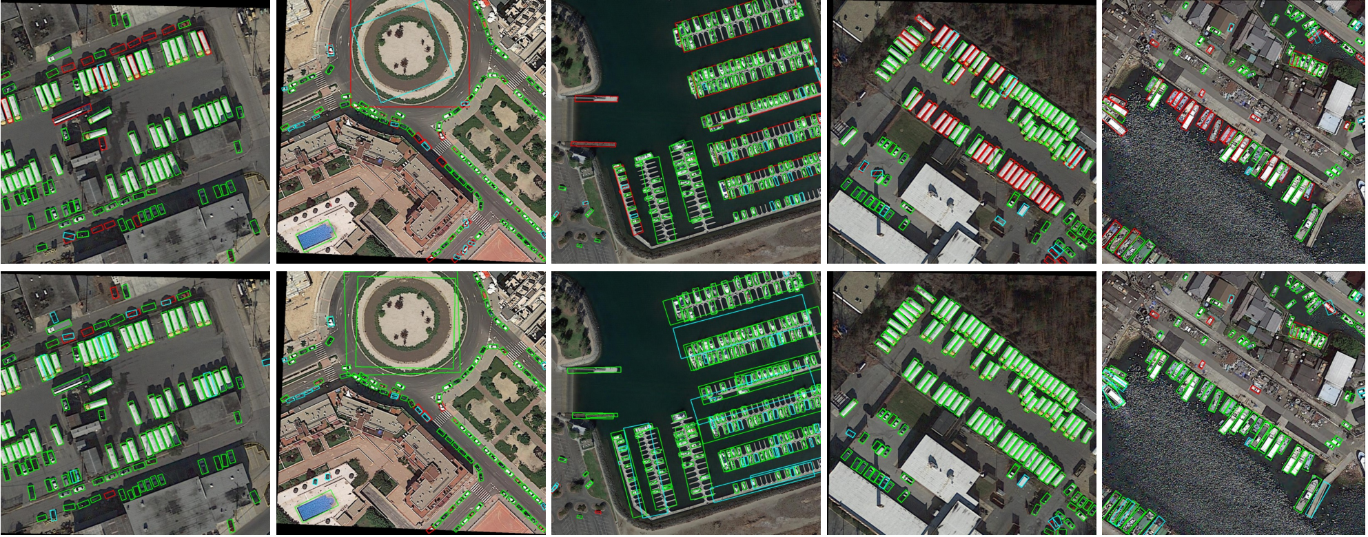
Visualization. We visualize the predicted results and positive samples in Fig. 5 and Fig. 7. We can see that the DCFL remarkably eliminates the False Negative and False Positive predictions, especially for the extreme-shaped oriented tiny objects. Fig. 7 shows that the proposed strategy is able to dynamically generate and sample priors that better fit the instance’s main body, verifying the claims of dynamic modeling and mismatch alleviation in this work.
Speed. We test the inference speed on DOTA-v2.0 val set with a single RTX3090 GPU, the FPS of the , -Net, RetinaNet, and DCFL is 16.2, 18.9, 20.8, and 20.9. It indicates that our method is of high efficiency. Moreover, we provide the parameters and GLOPs in Tab. 8, where we can see that the DCFL is lighter.
6 Conclusion
In this paper, we propose a novel DCFL scheme for detecting oriented tiny objects. We identify that the mismatched feature prior and unbalanced positive samples are two obstacles hampering the label assignment for oriented tiny objects. To address these, we propose a dynamic prior to alleviate the mismatch issue and a coarse-to-fine assigner to mitigate the imbalance issue, where the prior, label assignment, and gt representation are all reformulated in a dynamic manner. Extensive experiments and analyses show the convincing improvements brought by the DCFL.
Acknowledgement
We thank the reviewers for their comments. This work was supported in parts by NSFC (62271355, 62271354) and the Fundamental Research Funds for the Central Universities (2042022kf1010).
References
- (1) Yancheng Bai, Yongqiang Zhang, Mingli Ding, and Bernard Ghanem. Sod-mtgan: Small object detection via multi-task generative adversarial network. In European Conference on Computer Vision, pages 206–221. Springer, 2018.
- (2) Syed Muhammad Arsalan Bashir and Yi Wang. Small object detection in remote sensing images with residual feature aggregation-based super-resolution and object detector network. Remote Sensing, 13(9):1854, 2021.
- (3) Sean Bell, C Lawrence Zitnick, Kavita Bala, and Ross B Girshick. Inside-Outside Net: Detecting objects in context with skip pooling and recurrent neural networks. In IEEE Conference on Computer Vision and Pattern Recognition, pages 2874–2883, 2016.
- (4) Nicolas Carion, Francisco Massa, Gabriel Synnaeve, Nicolas Usunier, Alexander Kirillov, and Sergey Zagoruyko. End-to-end object detection with transformers. In European Conference on Computer Vision, pages 213–229. Springer, 2020.
- (5) Kai Chen, Jiangmiao Pang, Jiaqi Wang, Yu Xiong, Xiaoxiao Li, Shuyang Sun, Wansen Feng, Ziwei Liu, Jianping Shi, Wanli Ouyang, et al. Hybrid task cascade for instance segmentation. In IEEE Conference on Computer Vision and Pattern Recognition, pages 4974–4983, 2019.
- (6) Kai Chen, Jiaqi Wang, Jiangmiao Pang, and et al. MMDetection: Open mmlab detection toolbox and benchmark. CoRR, abs/arXiv:1906.07155, 2019.
- (7) Gong Cheng, Jiabao Wang, Ke Li, Xingxing Xie, Chunbo Lang, Yanqing Yao, and Junwei Han. Anchor-free oriented proposal generator for object detection. IEEE Transactions on Geoscience and Remote Sensing, 60:1–11, 2022.
- (8) Luc Courtrai, Minh-Tan Pham, and Sébastien Lefèvre. Small object detection in remote sensing images based on super-resolution with auxiliary generative adversarial networks. Remote Sensing, 12(19):3152, 2020.
- (9) Jifeng Dai, Haozhi Qi, Yuwen Xiong, Yi Li, Guodong Zhang, Han Hu, and Yichen Wei. Deformable convolutional networks. In IEEE Conference on Computer Vision and Pattern Recognition, pages 764–773, 2017.
- (10) Jian Ding, Nan Xue, Yang Long, Gui-Song Xia, and Qikai Lu. Learning roi transformer for detecting oriented objects in aerial images. In IEEE Conference on Computer Vision and Pattern Recognition, pages 2849–2858, 2019.
- (11) Jian Ding, Nan Xue, Gui-Song Xia, Xiang Bai, Wen Yang, Michael Ying Yang, Serge Belongie, Jiebo Luo, Mihai Datcu, Marcello Pelillo, et al. Object detection in aerial images: A large-scale benchmark and challenges. IEEE Transactions on Pattern Analysis and Machine Intelligence, 44(11):7778–7796, 2021.
- (12) Dawei Du, Pengfei Zhu, Longyin Wen, and et al. Visdrone-det2019: The vision meets drone object detection in image challenge results. In IEEE International Conference on Computer Vision Workshops, pages 213–226, 2019.
- (13) Dominik Maria Endres and Johannes E Schindelin. A new metric for probability distributions. IEEE Transactions on Information Theory (TIT), 49(7):1858–1860, 2003.
- (14) Zheng Ge, Songtao Liu, Zeming Li, Osamu Yoshie, and Jian Sun. Ota: Optimal transport assignment for object detection. IEEE Conference on Computer Vision and Pattern Recognition, 2021.
- (15) Spyros Gidaris and Nikos Komodakis. Object detection via a multi-region and semantic segmentation-aware cnn model. In IEEE Conference on Computer Vision and Pattern Recognition, pages 1134–1142, 2015.
- (16) Zonghao Guo, Chang Liu, Xiaosong Zhang, Jianbin Jiao, Xiangyang Ji, and Qixiang Ye. Beyond bounding-box: Convex-hull feature adaptation for oriented and densely packed object detection. In Proceedings of the IEEE/CVF Conference on Computer Vision and Pattern Recognition, pages 8792–8801, 2021.
- (17) Jiaming Han, Jian Ding, Jie Li, and Gui-Song Xia. Align deep features for oriented object detection. IEEE Transactions on Geoscience and Remote Sensing, 60:1–11, 2021.
- (18) Jiaming Han, Jian Ding, Nan Xue, and Gui-Song Xia. Redet: A rotation-equivariant detector for aerial object detection. In IEEE Conference on Computer Vision and Pattern Recognition, pages 2786–2795, 2021.
- (19) Kaiming He, Georgia Gkioxari, Piotr Dollar, and Ross Girshick. Mask R-CNN. In IEEE International Conference on Computer Vision, pages 2961–2969, 2017.
- (20) Kaiming He, Xiangyu Zhang, Shaoqing Ren, and Jian Sun. Deep residual learning for image recognition. In IEEE Conference on Computer Vision and Pattern Recognition, pages 770–778, 2016.
- (21) Liping Hou, Ke Lu, Jian Xue, and Yuqiu Li. Shape-adaptive selection and measurement for oriented object detection. In AAAI Conference on Artificial Intelligence, 2022.
- (22) Han Hu, Jiayuan Gu, Zheng Zhang, Jifeng Dai, and Yichen Wei. Relation networks for object detection. In IEEE Conference on Computer Vision and Pattern Recognition, pages 3588–3597, 2018.
- (23) Zhanchao Huang, Wei Li, Xiang-Gen Xia, and Ran Tao. A general gaussian heatmap label assignment for arbitrary-oriented object detection. IEEE Transactions on Image Processing, 31:1895–1910, 2022.
- (24) Kang Kim and Hee Seok Lee. Probabilistic anchor assignment with iou prediction for object detection. In European Conference on Computer Vision, pages 355–371. Springer, 2020.
- (25) Jianan Li, Xiaodan Liang, Yunchao Wei, Tingfa Xu, Jiashi Feng, and Shuicheng Yan. Perceptual generative adversarial networks for small object detection. In IEEE Conference on Computer Vision and Pattern Recognition, pages 1222–1230, 2017.
- (26) Wentong Li, Yijie Chen, Kaixuan Hu, and Jianke Zhu. Oriented reppoints for aerial object detection. In IEEE Conference on Computer Vision and Pattern Recognition, pages 1829–1838, 2022.
- (27) Yanghao Li, Yuntao Chen, Naiyan Wang, and Zhaoxiang Zhang. Scale-aware trident networks for object detection. In IEEE International Conference on Computer Vision, pages 6054–6063, 2019.
- (28) Zhonghua Li, Biao Hou, Zitong Wu, Licheng Jiao, Bo Ren, and Chen Yang. Fcosr: A simple anchor-free rotated detector for aerial object detection. arXiv preprint arXiv:2111.10780, 2021.
- (29) Tsung-Yi Lin, Piotr Dollar, Ross Girshick, Kaiming He, Bharath Hariharan, and Serge Belongie. Feature pyramid networks for object detection. In IEEE Conference on Computer Vision and Pattern Recognition, pages 2117–2125, 2017.
- (30) Tsung-Yi Lin, Priya Goyal, Ross Girshick, Kaiming He, and Piotr Dollar. Focal loss for dense object detection. In IEEE International Conference on Computer Vision, pages 2980–2988, 2017.
- (31) Tsung-Yi Lin, Michael Maire, Serge Belongie, James Hays, Pietro Perona, Deva Ramanan, Piotr Dollár, and C Lawrence Zitnick. Microsoft coco: Common objects in context. In European Conference on Computer Vision, pages 740–755. Springer, 2014.
- (32) Shilong Liu, Feng Li, Hao Zhang, Xiao Yang, Xianbiao Qi, Hang Su, Jun Zhu, and Lei Zhang. Dab-detr: Dynamic anchor boxes are better queries for detr. In International Conference on Learning Representations, 2021.
- (33) Shu Liu, Lu Qi, Haifang Qin, Jianping Shi, and Jiaya Jia. Path aggregation network for instance segmentation. In IEEE Conference on Computer Vision and Pattern Recognition, pages 8759–8768, 2018.
- (34) Wei Liu, Dragomir Anguelov, Dumitru Erhan, Christian Szegedy, Scott Reed, Cheng-Yang Fu, and Alexander C Berg. SSD: Single shot multibox detector. In European Conference on Computer Vision, pages 21–37. Springer, 2016.
- (35) Zikun Liu, Hongzhen Wang, Lubin Weng, and Yiping Yang. Ship rotated bounding box space for ship extraction from high-resolution optical satellite images with complex backgrounds. IEEE Geoscience and Remote Sensing Letters, 13(8):1074–1078, 2016.
- (36) Jianqi Ma, Weiyuan Shao, Hao Ye, Li Wang, Hong Wang, Yingbin Zheng, and Xiangyang Xue. Arbitrary-oriented scene text detection via rotation proposals. IEEE Transactions on Multimedia, 20(11):3111–3122, 2018.
- (37) Yuchen Ma, Songtao Liu, Zeming Li, and Jian Sun. Iqdet: Instance-wise quality distribution sampling for object detection. In Proceedings of the IEEE/CVF Conference on Computer Vision and Pattern Recognition, pages 1717–1725, 2021.
- (38) Qi Ming, Zhiqiang Zhou, Lingjuan Miao, Hongwei Zhang, and Linhao Li. Dynamic anchor learning for arbitrary-oriented object detection. In AAAI Conference on Artificial Intelligence, volume 35, pages 2355–2363, 2021.
- (39) Frank Nielsen. On a generalization of the jensen–shannon divergence and the jensen–shannon centroid. Entropy, 22(2):221, 2020.
- (40) Junhyug Noh, Wonho Bae, Wonhee Lee, Jinhwan Seo, and Gunhee Kim. Better to follow, follow to be better: Towards precise supervision of feature super-resolution for small object detection. In IEEE International Conference on Computer Vision, pages 9725–9734, 2019.
- (41) Adam Paszke, Sam Gross, Francisco Massa, Adam Lerer, et al. Pytorch: An imperative style, high-performance deep learning library. In Advances in Neural Information Processing Systems, pages 8024–8035, 2019.
- (42) Siyuan Qiao, Liang-Chieh Chen, and Alan Yuille. Detectors: Detecting objects with recursive feature pyramid and switchable atrous convolution. In IEEE Conference on Computer Vision and Pattern Recognition, 2021.
- (43) Jakaria Rabbi, Nilanjan Ray, Matthias Schubert, Subir Chowdhury, and Dennis Chao. Small-object detection in remote sensing images with end-to-end edge-enhanced gan and object detector network. Remote Sensing, 12(9):1432, 2020.
- (44) Shaoqing Ren, Kaiming He, Ross Girshick, and Jian Sun. Faster R-CNN: Towards real-time object detection with region proposal networks. In Advances in Neural Information Processing Systems, pages 91–99, 2015.
- (45) Olga Russakovsky, Jia Deng, Hao Su, Jonathan Krause, Sanjeev Satheesh, Sean Ma, Zhiheng Huang, Andrej Karpathy, Aditya Khosla, Michael Bernstein, et al. Imagenet large scale visual recognition challenge. International Journal of Computer Vision, 115(3):211–252, 2015.
- (46) Bharat Singh and Larry S Davis. An analysis of scale invariance in object detection snip. In IEEE Conference on Computer Vision and Pattern Recognition, pages 3578–3587, 2018.
- (47) Bharat Singh, Mahyar Najibi, and Larry S Davis. Sniper: Efficient multi-scale training. In Advances in Neural Information Processing Systems, pages 9310–9320, 2018.
- (48) Peize Sun, Rufeng Zhang, Yi Jiang, Tao Kong, Chenfeng Xu, Wei Zhan, Masayoshi Tomizuka, Lei Li, Zehuan Yuan, Changhu Wang, and Ping Luo. Sparse r-cnn: End-to-end object detection with learnable proposals. In IEEE Conference on Computer Vision and Pattern Recognition, pages 14454–14463, 2021.
- (49) Mingxing Tan, Ruoming Pang, and Quoc V Le. Efficientdet: Scalable and efficient object detection. In IEEE Conference on Computer Vision and Pattern Recognition, pages 10781–10790, 2020.
- (50) Zhi Tian, Chunhua Shen, Hao Chen, and Tong He. FCOS: Fully convolutional one-stage object detection. In IEEE International Conference on Computer Vision, pages 9627–9636, 2019.
- (51) Zhi Tian, Chunhua Shen, Hao Chen, and Tong He. Fcos: A simple and strong anchor-free object detector. IEEE Transactions on Pattern Analysis and Machine Intelligence, 2020.
- (52) Jiaqi Wang, Kai Chen, Shuo Yang, Chen Change Loy, and Dahua Lin. Region proposal by guided anchoring. In IEEE Conference on Computer Vision and Pattern Recognition, pages 2965–2974, 2019.
- (53) Jinwang Wang, Wen Yang, Heng-chao Li, Haijian Zhang, and Gui-Song Xia. Learning center probability map for detecting objects in aerial images. IEEE Transactions on Geoscience and Remote Sensing, 59(5):4307–4323, 2021.
- (54) Yingming Wang, Xiangyu Zhang, Tong Yang, and Jian Sun. Anchor detr: Query design for transformer-based detector. In AAAI Conference on Artificial Intelligence, volume 36, pages 2567–2575, 2022.
- (55) Gui-Song Xia, Xiang Bai, Jian Ding, Zhen Zhu, Serge Belongie, Jiebo Luo, Mihai Datcu, Marcello Pelillo, and Liangpei Zhang. DOTA: A large-scale dataset for object detection in aerial images. In IEEE Conference on Computer Vision and Pattern Recognition, pages 3974–3983, 2018.
- (56) Xingxing Xie, Gong Cheng, Jiabao Wang, Xiwen Yao, and Junwei Han. Oriented r-cnn for object detection. In IEEE International Conference on Computer Vision, pages 3520–3529, 2021.
- (57) Chang Xu, Jinwang Wang, Wen Yang, Huai Yu, Lei Yu, and Gui-Song Xia. Detecting tiny objects in aerial images: A normalized wasserstein distance and a new benchmark. In ISPRS Journal of Photogrammetry and Remote Sensing, volume 190, pages 79–93, 2022.
- (58) Chang Xu, Jinwang Wang, Wen Yang, Huai Yu, Lei Yu, and Gui-Song Xia. Rfla: Gaussian receptive field based label assignment for tiny object detection. In European Conference on Computer Vision, pages 526–543. Springer, 2022.
- (59) Chang Xu, Jinwang Wang, Wen Yang, and Lei Yu. Dot distance for tiny object detection in aerial images. In IEEE Conference on Computer Vision and Pattern Recognition Workshops, pages 1192–1201, 2021.
- (60) Xue Yang, Qingqing Liu, Junchi Yan, Ang Li, Zhiqiang Zhang, and Gang Yu. R3det: Refined single-stage detector with feature refinement for rotating object. CoRR, abs/arXiv:1908.05612, 2019.
- (61) Xue Yang, Junchi Yan, Qi Ming, Wentao Wang, Xiaopeng Zhang, and Qi Tian. Rethinking rotated object detection with gaussian wasserstein distance loss. In International Conference on Machine Learning, volume 139, pages 11830–11841, 2021.
- (62) Xue Yang, Jirui Yang, Junchi Yan, Yue Zhang, Tengfei Zhang, Zhi Guo, Xian Sun, and Kun Fu. SCRDet: Towards more robust detection for small, cluttered and rotated objects. In IEEE International Conference on Computer Vision, pages 8232–8241, 2019.
- (63) Xue Yang, Xiaojiang Yang, Jirui Yang, Qi Ming, Wentao Wang, Qi Tian, and Junchi Yan. Learning high-precision bounding box for rotated object detection via kullback-leibler divergence. Advances in Neural Information Processing Systems, 34, 2021.
- (64) Xue Yang, Gefan Zhang, Xiaojiang Yang, Yue Zhou, Wentao Wang, Jin Tang, Tao He, and Junchi Yan. Detecting rotated objects as gaussian distributions and its 3-d generalization. IEEE Transactions on Pattern Analysis and Machine Intelligence, 2022.
- (65) Ze Yang, Shaohui Liu, Han Hu, Liwei Wang, and Stephen Lin. Reppoints: Point set representation for object detection. In IEEE International Conference on Computer Vision, pages 9657–9666, 2019.
- (66) Jiahui Yu, Yuning Jiang, Zhangyang Wang, Zhimin Cao, and Thomas Huang. Unitbox: An advanced object detection network. pages 516–520, 2016.
- (67) Mohsen Zand, Ali Etemad, and Michael Greenspan. Objectbox: From centers to boxes for anchor-free object detection. European Conference on Computer Vision, 2022.
- (68) Shifeng Zhang, Cheng Chi, Yongqiang Yao, Zhen Lei, and Stan Z Li. Bridging the gap between anchor-based and anchor-free detection via adaptive training sample selection. In IEEE Conference on Computer Vision and Pattern Recognition, pages 9759–9768, 2020.
- (69) Qijie Zhao, Tao Sheng, Yongtao Wang, Zhi Tang, Ying Chen, Ling Cai, and Haibin Ling. M2det: A single-shot object detector based on multi-level feature pyramid network. In AAAI Conference on Artificial Intelligence, pages 9259–9266, 2019.
- (70) Yue Zhou, Xue Yang, Gefan Zhang, Jiabao Wang, Yanyi Liu, Liping Hou, Xue Jiang, Xingzhao Liu, Junchi Yan, Chengqi Lyu, et al. Mmrotate: A rotated object detection benchmark using pytorch. arXiv preprint arXiv:2204.13317, 2022.
- (71) Chenchen Zhu, Yihui He, and Marios Savvides. Feature selective anchor-free module for single-shot object detection. In IEEE Conference on Computer Vision and Pattern Recognition, pages 840–849, 2019.
- (72) Xizhou Zhu, Weijie Su, Lewei Lu, Bin Li, Xiaogang Wang, and Jifeng Dai. Deformable detr: Deformable transformers for end-to-end object detection. In International Conference on Learning Representations, 2021.