Two-stage Denoising Diffusion Model for Source Localization in Graph Inverse Problems

Diffusion models aim to approximate the prior distributions by learning the noise of the data reversely. [12] combines SMLD [14] and DDPM [11] into a generalized theoretical framework, known as the Score-Based Diffusion Model. They generally map data to a noise distribution (the prior) with a stochastic differential equation (SDE), and reverse this SDE for generative modeling.

The graph information dissemination problem involves a graph $G=(V,E)$ with edge set $E$ and node set $V$. An information dissemination cascade $D_{i}$ at length $K+1$ on the graph is defined as $D_{i}=\left\{\left(v_{i_{k}},k\right)\mid v_{i_{k}}\in V,k=0,1\ldots,K-1,K\right\}$, where $k$ is non-decreasing and the first $K_{s}$ nodes are defined as source nodes. The source indicator $\mathbf{i}\in\{0,1\}^{|V|}$ is defined as $0$ for being the source and $1$ for not, while the source proximity degree $\mathbf{x}\in[0,1]^{|V|}$ is defined as $x_{k}=\frac{k}{K}$. The set of affected nodes’ observations is denoted as $\mathbf{y}\in\{0,1\}^{|V|}$, where $0$ indicates being affected and $1$ indicates not being affected. The goal of the graph information dissemination problem is to predict the affected nodes given the source indicator and graph structure.

Thanks to the outstanding performance of GNN on graph data, the state-of-the-art graph information dissemination methods [1, 4, 3, 26] construct various realistic-meaning attribute variables through GNN at the first stage, and then perform variable dissemination to derive the final affected node sets. Specifically: (1) In the variable construction, we define a neural network $\mathbf{v}=g_{\mathbf{w_{1}}}(\mathbf{x})$ to construct miscellaneous variables of nodes (such as sender variable or receiver variable). (2) In variable dissemination, we define a dissemination neural network $f_{\mathbf{w_{2}}}(\mathbf{v})$ to propagate information to neighbour nodes according to the topology of the graph, where $w_{1}$ and $w_{2}$ are learnable parameters. Thus, the general paradigm of graph information dissemination can be defined as:

In order to eliminate ambiguity, the graph mentioned in Subsection 3.2 is referred to as the whole graph $\mathcal{G}^{w}=(V^{w},E^{w})$. Source localization is the corresponding inverse problem of graph information dissemination, which is formally defined as: given the whole graph information $\mathcal{G}^{w}=(V^{w},E^{w})$ and affected nodes $\mathbf{y}\in\{0,1\}^{|V|}$, reconstruct the source nodes $\mathbf{\hat{i}}\in\{0,1\}^{|V|}$. For the convenience of mentioning later, we define the cascade graph as $\mathcal{G}^{c}_{i}=(V^{c}_{i}\in D_{i},E^{c})$ where $E^{c}=\{(u,v)\in E^{w}\mid u\in D_{i}\text{ or }v\in D_{i}\}$.

To mitigate the computational burden of simulating information dissemination on the whole graph at each diffusion step (chall. 3), and to leverage the cascade temporal information for addressing the ill-posed problem (chall. 3), we propose a two-stage optimization framework, as depicted in Figure 5. Specifically, in the coarse stage, the supervising signals for the model are the source proximity degrees (Figure 3(a)) that fully retain the cascade temporal information. In other words, the final outputs of this stage are the relatively coarse-grained node infection sequence predictions, which are used to initialize the precise source localization for the next stage efficiently. In the second stage, i.e., the fine stage, the supervising signals of model training are source indicators (Figure 3(b)), which aim to accurately output the predicted source under the given disseminated observation conditions. In this stage, the model simulates the information dissemination on the graph at each diffusion step to calibrate predictions.

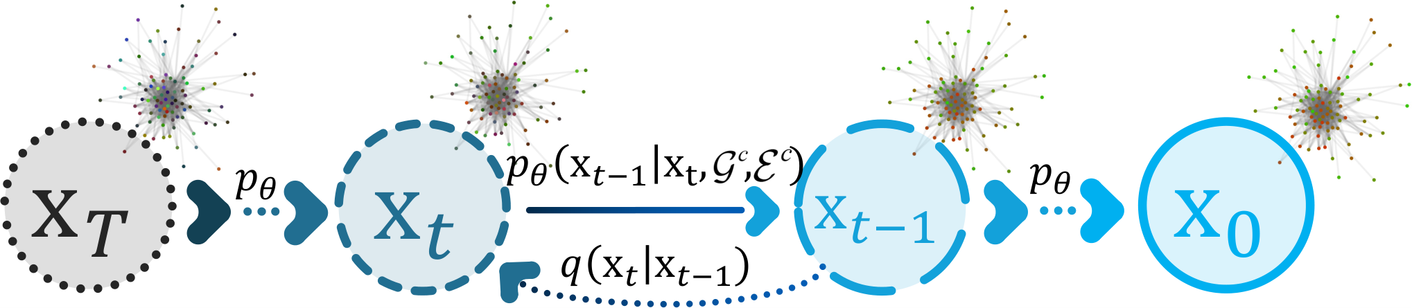
In this section, we propose a coarse proximity generation model at the first stage, which serves to effectively initialize the subsequent stage. The “coarse” is used in two senses. Firstly, the source proximity degree derived from the cascade data does not strictly reflect the infection relationships between nodes, as the nodes in a cascade may be infected by their common ancestors rather than by their directly adjacent forward nodes. Secondly, as no dissemination model is incorporated at this stage, it is not feasible to accurately predict the dissemination source in reverse. Nonetheless, the generated coarse source proximity degrees are well-suited for the initialization of the downstream diffusion model. Although the coarse source proximity generation occurs only within the cascade graph, it is incomplete without considering the structure of the entire graph. This is due to the significant impact that the relative position of each node in the graph has on information dissemination. To address this, we utilize Position-aware Graph Neural Networks (P-GNN) [27] to perform node position representation learning on the whole graph of each dataset. Through this process, we obtain the positional embeddings $\mathcal{E}^{w}=\{\mathbf{e}_{i}\mid\mathbf{e}_{i}=\text{P-GNN}(v_{i}),v_{i}\in V^{w}\}$ that reflect the relative position of each node with respect to other nodes on the whole graph. We use this positional representation in the specific cascade $\mathcal{E}^{c}=\{\mathbf{e}_{i}\mid\mathbf{e}_{i}=\text{P-GNN}(v_{i}),v_{i}\in V^{c}\}$ as a conditional input to the score function approximation network, enhancing its ability to fit the underlying features of the cascades.

Let the original source proximity degrees derived from a cascade be denoted as $\mathbf{x}_{0}$. The reverse SDE here follows the Equation 2, while the score function conditioned on the the cascade graph structure and the positional embeddings is changed to $\mathbf{s}_{\boldsymbol{\theta}}(\mathbf{x}_{t},t\mid\mathcal{G}^{c},\mathcal{E}^{c})$. We adopt the same variance schedule as DDPM [11] to discretize the formula, then the estimated reverse Markov chain is defined as follows:

in which we use the following re-weighted variant of the evidence lower bound (ELBO) to train the model to obtain the estimated score function:

where $\alpha:=\prod^{i}_{j=1}(1-\beta_{j})$.

To efficiently approximate the score functions, we propose a new network structure that properly introduces conditional position embeddings while preserving nodes’ adjacent characteristics at different orders. Our approach utilizes a multi-head graph attention (GMT) [28] as the basic operation of graph convolution, allowing us to aggregate information across $L$-layer graphs. Furthermore, we leverage skip connections between each layer to improve the flow of information. Finally, we concatenate the output of each layer and perform multi-layer nonlinear transformations to obtain an estimated score function. The proposed conditional score function approximating network is defined as follows:

where $\mathbf{H}^{0}=\mathbf{x}_{t}+\mathcal{E}^{c}$. We use the positional encodings [29] to encode the diffusion step, and the formula is defined as: $\mathcal{T}(t)=\left[\ldots,\cos\left(t/r^{\frac{-2d}{D}}\right),\sin\left(t/r^{\frac{-2d}{D}}\right),\ldots\right]^{\mathrm{T}}$, where $d=1,\dots,D/2$ is the dimension of the embedding, and r is a large constant (set to $10^{5}$). After obtaining the trained network $\mathbf{s}_{\boldsymbol{\theta}}$, we sample according to the Algorithm 1 and get the predicted coarse source proximity degrees.

In the second stage, we apply the estimated source proximity degree to initialize the graph dissemination conditioned diffusion model. Significantly different from the conditional diffusion in the first stage, the diffusion model here is an inverse problem solver, which aims to recover the source indicator $\mathbf{i}$ from the disseminated observation $\mathbf{y}$. The connection between them is the forward information dissemination process of $\mathbf{i}\rightarrow\mathbf{y}$.

If the assumption is the same as in [12], that is, $p_{t}\left(\mathbf{y}\mid\mathbf{i}_{t}\right)$ is tractable, then the reverse SDE of the inverse problem is defined as:

However, in our case, $p_{t}\left(\mathbf{y}\mid\mathbf{i}_{t}\right)$ is intractable, as the dissemination model cannot support the source with noise as input. To bridge this gap, we introduce the approximation method [13] for $p(\hat{\mathbf{i}_{0}}\mid\mathbf{i}_{t})$:

where $\alpha_{i}\triangleq 1-\beta_{i},\bar{\alpha}_{i}\triangleq\prod_{j=1}^{i}\alpha_{i}$ following [11]. Now the problem lies in determining an appropriate dissemination model to calculate the posterior probability of $\mathbf{y}$ from estimated $\mathbf{i}$. In real-world applications, various random factors can impact the information dissemination process, which are not accounted for in the basic dissemination function (Equation 4). Our proposed model addresses this challenge by qualifying the uncertain trough Gaussian noise $\tilde{\sigma}(t)$ with adaptive variance (parameterized by MLP and taking diffusion step as input). Additionally, our model can eliminate interference from noise to source localization through the powerful iterative denoising process of the diffusion model. Thus, the formula is defined as follows:

From the above formula, we can calculate the partial derivative $\nabla_{\mathbf{i}_{0}}\log p\left(\mathbf{y}\mid\mathbf{i}_{0}\right)$. And bring the conclusion in Equation 8 into it to get an approximate for the derivative of $p\left(\mathbf{y}\mid\mathbf{i}_{t}\right)$ with respect to $\hat{\mathbf{i}_{t}}$.

Hence, we can discretize Equation 8 similarly to formula 5 and deduce the expression for $p(\mathbf{i}_{t-1})\mid\mathbf{i}_{t})$. This allows us to perform iterative denoising of $\mathbf{i}$ given the posterior $\mathbf{y}$, ultimately leading to an accurate estimation of $\mathbf{i}$. For a more thorough explanation of this procedure, please refer to Algorithm 2. 0:  ground truth source proximity degree ${\mathbf{x}}$, number of diffusion steps $T_{1}$, variance schedule $\beta_{t}$, the cascade graph $\mathcal{G}_{c}$ 1:  $\mathbf{x}_{T_{1}}\sim\mathcal{N}(\mathbf{0,I})$ 2:  for $t=T_{1}-1$ to $t=0$ do 3:   $\hat{\mathbf{s}}\leftarrow\mathbf{s}_{\boldsymbol{\phi}}(\mathbf{x}_{t},t\mid\mathcal{G}^{w},\mathcal{E}^{w})$ 4:   $\mathbf{x}_{t-1}^{\prime}\leftarrow(2-\sqrt{1-\beta_{t}}\mathbf{x}_{t})+\beta_{t}\left(\hat{\mathbf{s}}\right)$ 5:   $\mathbf{z}\sim\mathcal{N}(\mathbf{0,I})$ 6:   $\mathbf{x}_{t}\leftarrow\mathbf{x}_{t-1}^{\prime}+\sqrt{\beta_{t}}\mathbf{z}$ 7:  end for 8:  return the estimated $\mathbf{x}_{0}$ Algorithm 1 Sampling of the coarse stage 0:  disseminated observation $\mathbf{y}$, coarse source proximity degree $\hat{\mathbf{x}}$, number of diffusion steps $T_{2}$, variance schedule $\beta_{t}$, the whole graph $\mathcal{G}_{W}$ 1:  $\mathbf{i}_{T_{2}}\leftarrow\hat{\mathbf{x}}$ 2:  for $t=T_{2}-1$ to $t=0$ do 3:   $\hat{\mathbf{s}}\leftarrow\mathbf{s}_{\boldsymbol{\phi}}(\mathbf{i}_{t},t\mid\mathcal{G}^{w})$ 4:   $\mathbf{i}_{t-1}^{\prime}\leftarrow(2-\sqrt{1-\beta_{t}}\mathbf{i}_{t})+\beta_{t}\left(\hat{\mathbf{s}}-\frac{1}{{\tilde{\sigma}(t)}^{2}}\nabla_{\mathbf{i}_{t}}\left\|\mathbf{y}-\hat{\mathbf{y}}\left(\hat{\mathbf{i}}_{0}\left(\mathbf{i}_{t}\right)\right)\right\|_{2}^{2}\right)$ 5:   $\mathbf{z}\sim\mathcal{N}(\mathbf{0,I})$ 6:   $\mathbf{i}_{t}\leftarrow\mathbf{i}_{t-1}^{\prime}+\sqrt{\beta_{t}}\mathbf{z}$ 7:  end for 8:  return the estimated $\mathbf{i}_{0}$ Algorithm 2 Sampling of the fine stage

We have conducted in-depth comparisons of SL-Diff with state-of-the-art baselines on five real datasets, and the results are presented in Table 1. Generally, models with preset dissemination modes perform relatively poorly, as real information dissemination modes are complex and full of uncertainties. SL-Diff, on the other hand, achieves significantly optimal results in most cases. Among them, the improvement on the Twitter and Android datasets is particularly significant which can be attributed to its ability to denoise the dissemination noise. And this noise is more prominent on datasets with a large cascade length and a large number of nodes. Correspondingly, on the Christianity dataset with a small number of nodes, the performance of SL-Diff is limited. In summary, SL-Diff is more capable of handling large-scale datasets.

To verify the effectiveness of each component of our proposed model, we conduct the following ablation experiments. Compared with the complete model, SL-Diff(1) only retains the coarse stage and is initialized randomly. SL-Diff(2) only retains the fine stage and we take the top 5% of nodes with the largest source proximity degree generated as the source of prediction. SL-Diff(3) is the model with the cascade positional representations removed, and SL-Diff(4) removes the simulated dissemination noise term in Equation 10. The diffusion step of the above four models is all set to 800. From the results in Table 2, we can conclude that only the coarse stage model can make rough predictions to a certain extent, and it is difficult to make accurate predictions. The model with only the fine stage is not necessarily more accurate than the two-stage model, and the computational overhead is huge, which is not feasible. From the results of SL-Diff(3), we can see that cascade positional representations generally have a more important influence on larger-scale graphs, which may be due to the fact that the relative position of cascades in large-scale graphs will be more complicated, and their influence on propagation will be larger. From the results of SL-Diff(4), we can find that simulated dissemination noise improves the model with a longer cascade length more significantly, which may be because a cascade with a longer propagation chain will introduce relatively more noise.

In this section, we explore the interdependence of the two stages in greater detail. Specifically, we set the ratio of the diffusion step of the fine stage to the coarse stage as $R_{T}=\frac{T_{2}}{T_{1}}$ and keep the total diffusion step at 800. By adjusting the value of $R_{T}$, we gain a deeper understanding of how the two stages mutually reinforce each other, and determine the optimal ratio. As shown in Figure 8, we observe that the model’s performance initially improves significantly with an increasing proportion of the fine stage, but then gradually declines, while the sampling time steadily increases. This suggests that we can identify the most suitable ratio of the two stages at a relatively low time cost across different datasets. The performance degradation resulting from too high $R_{T}$ may be due to insufficient denoising in the coarse stage. Additionally, we analyze the impact of the diffusion step on the model’s performance under the configuration with the optimal $R_{T}$. Figure 9 reveals that the convergence of the sampling process is comparatively faster for datasets with smaller scales.

References

- [1] Aravind Sankar, Xinyang Zhang, Adit Krishnan, and Jiawei Han. Inf-vae: A variational autoencoder framework to integrate homophily and influence in diffusion prediction. In Proceedings of the 13th international conference on web search and data mining, pages 510–518, 2020.
- [2] Wenwen Xia, Yuchen Li, Jun Wu, and Shenghong Li. Deepis: Susceptibility estimation on social networks. In Proceedings of the 14th ACM International Conference on Web Search and Data Mining, pages 761–769, 2021.
- [3] Shanshan Feng, Kaiqi Zhao, Lanting Fang, Kaiyu Feng, Wei Wei, Xutao Li, and Ling Shao. H-diffu: Hyperbolic representations for information diffusion prediction. IEEE Transactions on Knowledge and Data Engineering, 2022.
- [4] Ruijie Wang, Zijie Huang, Shengzhong Liu, Huajie Shao, Dongxin Liu, Jinyang Li, Tianshi Wang, Dachun Sun, Shuochao Yao, and Tarek Abdelzaher. Dydiff-vae: A dynamic variational framework for information diffusion prediction. In Proceedings of the 44th International ACM SIGIR Conference on Research and Development in Information Retrieval, pages 163–172, 2021.
- [5] Zheng Wang, Chaokun Wang, Jisheng Pei, and Xiaojun Ye. Multiple source detection without knowing the underlying propagation model. In Proceedings of the AAAI Conference on Artificial Intelligence, volume 31, 2017.
- [6] Ming Dong, Bolong Zheng, Nguyen Quoc Viet Hung, Han Su, and Guohui Li. Multiple rumor source detection with graph convolutional networks. In Proceedings of the 28th ACM international conference on information and knowledge management, pages 569–578, 2019.
- [7] Junxiang Wang, Junji Jiang, and Liang Zhao. An invertible graph diffusion neural network for source localization. In Proceedings of the ACM Web Conference 2022, pages 1058–1069, 2022.
- [8] Zhen Wang, Dongpeng Hou, Chao Gao, Jiajin Huang, and Qi Xuan. A rapid source localization method in the early stage of large-scale network propagation. In Proceedings of the ACM Web Conference 2022, pages 1372–1380, 2022.
- [9] Chen Ling, Junji Jiang, Junxiang Wang, and Zhao Liang. Source localization of graph diffusion via variational autoencoders for graph inverse problems. In Proceedings of the 28th ACM SIGKDD Conference on Knowledge Discovery and Data Mining, pages 1010–1020, 2022.
- [10] Kai Zhu, Zhen Chen, and Lei Ying. Catch’em all: Locating multiple diffusion sources in networks with partial observations. In Thirty-First AAAI Conference on Artificial Intelligence, 2017.
- [11] Jonathan Ho, Ajay Jain, and Pieter Abbeel. Denoising diffusion probabilistic models. Advances in Neural Information Processing Systems, 33:6840–6851, 2020.
- [12] Yang Song, Jascha Sohl-Dickstein, Diederik P Kingma, Abhishek Kumar, Stefano Ermon, and Ben Poole. Score-based generative modeling through stochastic differential equations. In International Conference on Learning Representations, 2021.
- [13] Hyungjin Chung, Jeongsol Kim, Michael T Mccann, Marc L Klasky, and Jong Chul Ye. Diffusion posterior sampling for general noisy inverse problems. arXiv preprint arXiv:2209.14687, 2022.
- [14] Yang Song, Sahaj Garg, Jiaxin Shi, and Stefano Ermon. Sliced score matching: A scalable approach to density and score estimation. In Uncertainty in Artificial Intelligence, pages 574–584. PMLR, 2020.
- [15] Minkai Xu, Lantao Yu, Yang Song, Chence Shi, Stefano Ermon, and Jian Tang. Geodiff: A geometric diffusion model for molecular conformation generation. In International Conference on Learning Representations, 2021.
- [16] David Kempe, Jon Kleinberg, and Eva Tardos. Maximizing the spread of influence through a social network. In Proceedings of the ninth ACM SIGKDD international conference on Knowledge discovery and data mining, pages 137–146, 2003.
- [17] Matt J Keeling and Ken TD Eames. Networks and epidemic models. Journal of the royal society interface, 2(4):295–307, 2005.
- [18] Mohamed Ahmed, Stella Spagna, Felipe Huici, and Saverio Niccolini. A peek into the future: Predicting the evolution of popularity in user generated content. In Proceedings of the sixth ACM international conference on Web search and data mining, pages 607–616, 2013.
- [19] Yongqing Wang, Huawei Shen, Shenghua Liu, Jinhua Gao, and Xueqi Cheng. Cascade dynamics modeling with attention-based recurrent neural network. In IJCAI, volume 17, pages 2985–2991, 2017.
- [20] Jiayi Xie, Yaochen Zhu, Zhibin Zhang, Jian Peng, Jing Yi, Yaosi Hu, Hongyi Liu, and Zhenzhong Chen. A multimodal variational encoder-decoder framework for micro-video popularity prediction. In Proceedings of The Web Conference 2020, pages 2542–2548, 2020.
- [21] Kai Zhu and Lei Ying. Information source detection in the sir model: A sample-path-based approach. IEEE/ACM Transactions on Networking, 24(1):408–421, 2014.
- [22] Diederik P Kingma and Max Welling. Auto-encoding variational bayes. Int. Conf. on Learning Representations, 2013.
- [23] Jaehyeong Jo, Seul Lee, and Sung Ju Hwang. Score-based generative modeling of graphs via the system of stochastic differential equations. arXiv preprint arXiv:2202.02514, 2022.
- [24] Kashif Rasul, Calvin Seward, Ingmar Schuster, and Roland Vollgraf. Autoregressive denoising diffusion models for multivariate probabilistic time series forecasting. In International Conference on Machine Learning, pages 8857–8868. PMLR, 2021.
- [25] Brian DO Anderson. Reverse-time diffusion equation models. Stochastic Processes and their Applications, 12(3):313–326, 1982.
- [26] Ling Sun, Yuan Rao, Xiangbo Zhang, Yuqian Lan, and Shuanghe Yu. Ms-hgat: Memory-enhanced sequential hypergraph attention network for information diffusion prediction. 2022.
- [27] Jiaxuan You, Rex Ying, and Jure Leskovec. Position-aware graph neural networks. In International conference on machine learning, pages 7134–7143. PMLR, 2019.
- [28] Jinheon Baek, Minki Kang, and Sung Ju Hwang. Accurate learning of graph representations with graph multiset pooling. arXiv preprint arXiv:2102.11533, 2021.
- [29] Ashish Vaswani, Noam Shazeer, Niki Parmar, Jakob Uszkoreit, Llion Jones, Aidan N Gomez, Łukasz Kaiser, and Illia Polosukhin. Attention is all you need. Advances in neural information processing systems, 30, 2017.
- [30] B Aditya Prakash, Jilles Vreeken, and Christos Faloutsos. Spotting culprits in epidemics: How many and which ones? In 2012 IEEE 12th International Conference on Data Mining, pages 11–20. IEEE, 2012.