Contact Tracing over Uncertain Indoor Positioning Data (Extended Version)

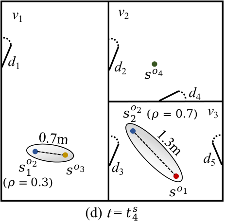
In our setting, an indoor positioning system aperiodically reports an indoor moving object $o$’s positioning record as $\psi=(l,t,et)$, which means that object $o$ was found at a location $l$ at time $t$ and the result is expired at a later time $et$. A location $l$ is captured as $(x,y,f)$, meaning a point $(x,y)$ on a floor $f$. Each object $o$’s raw trajectory $\Psi_{o}$ is a time-ordered sequence of all its positioning records. In such a raw trajectory $\Psi_{o}$, two consecutive positioning records $\psi_{i}=(l_{i},t_{i},et_{i})$ and $\psi_{i+1}=(l_{i+1},t_{i+1},et_{i+1})$ satisfy that $et_{i}<t_{i+1}$. Due to the discrete nature of indoor positioning, the records of an indoor trajectory $\Psi_{o}$ most often do not fully disclose the object whereabouts during $\Psi_{o}$’s lifespan.

To enable the comparison of two objects’ trajectories throughout a common part of their lifespans, we generate the sampled trajectory of each object as follows. First, we set a unified sampling time interval $\Delta t$, and sample the object locations at each sampling time $t^{s}_{w}=t_{o}+w\cdot\Delta t$ where $t_{o}$ is the global origin time and $w$ is a non-negative integer. Subsequently, the location sample at each sampling time $t^{s}_{w}$ is generated in two cases. If $t^{s}_{w}$ falls within the time range $[t_{i},et_{i}]$ of a record $\psi_{i}$, a sample $s=(l_{i},1)$ is generated, meaning that $o$ is located at $l_{i}$ with the probability of 1. Such a sample is directly obtained from the raw positioning record and thus is called an original sample. Otherwise, the two positioning records before and after the sampling time $t^{s}_{w}$ are obtained, and a set $S_{w}$ of samples in the form of $s_{i}=(l_{i},\rho_{i})$ are derived based on the two obtained positioning records. Such a sample is called a derived sample. Each sampled location $l_{i}$ is associated with a probability $\rho_{i}$ and we have $\sum_{s_{i}\in S_{w}}s_{i}.\rho_{i}=1$. How to obtain the location samples based on the contextual positioning records will be detailed in Section III-C.

As a result, a sampled trajectory $\Psi^{s}_{o}$ is obtained as the time-ordered sequence of the sample sets at all sampling times, formally $\langle(S_{1},t^{s}_{1}),\ldots,(S_{W},t^{s}_{W})\rangle$. In this way, all objects’ location samples are aligned in the time dimension and the comparison of objects is performed only at the sampling times. Note that an object’s sampled trajectory is only generated within the lifespan of its raw trajectory.

In real applications, it is interesting to find out those moving objects that had very close contact with a particular object for a sufficiently long period of time, equivalently a sufficient number of consecutive sampling times from the perspective of sampled trajectories. In this paper, we propose a self-contained set of contact tracing techniques that allow us to efficiently find close contacts to a given object by using uncertain indoor positioning data.

We first define the contact distance as follows.

In the definition above, a partition refers to a basic topological unit of the indoor space, e.g., rooms, staircases, and elevators. Two persons are not considered contact if they are in different partitions²² 2 In certain situations, objects located near a door but in separate partitions, such as $s^{o_{1}}$ and $s^{o_{4}}$ in Fig. 1, may be considered in contact. Our method can be easily adapted to cover this case by linking an object near a door within a certain distance to both adjacent partitions in the proposed enhanced indoor graph model in Section III-A.. For example, in Fig. 1 (a), the contact distance between $s^{o_{2}}$ and $s^{o_{3}}$ is the Euclidean distance $1.9$ meters, while the contact distance between $s^{o_{2}}$ and $s^{o_{4}}$ is infinite because they are not in the same partition. Given the distance threshold $\delta$ in contact restriction, two objects’ contact probability at a sampling time $t^{s}_{w}$ is defined as follows.

We say two objects are instant contact with each other at time $t$ if their contact probability is higher than a specified threshold $\eta$.

Finally, our research problem is formulated as follows.

Fig. 3 shows our solution for ICQ. The bottom layer lays the technical foundations of ICQ processing, as to be detailed in Section III. In particular, an enhanced graph model is constructed to accommodate the indoor space data, indoor moving objects, and sampled trajectories for relevant computations. On top of the enhanced graph model, it first finds a moving object’s uncertainty region, i.e., the object’s possible locations at a sampling time. Based on the uncertainty regions, it derives samples which in turn are maintained in the enhanced graph model for subsequent use.

To process a query instance $\textsc{ICQ}{}(o,T,\delta,\eta,k)$, an overall framework is proposed as Algorithm 3. It finds all objects in close contact with the query object $o$ by calling Algorithm 4 (the constrained search), which employs a set of strategies for acceleration. Then, Algorithm 4 calls Algorithm 1 to determine the instant close contact and further help set the start timestamp. It also calls Algorithm 2 for close contact determination when processing a candidate object. Algorithm 2 calls Algorithm 1 to compute the contact probability at an instant timestamp. We present the close contact determination in Section IV-A and the ICQ search in Section IV-B.

It is noteworthy that Algorithms 1 calls a Derive Sample function when computing contact probabilities over object samples, whose details can be found in Appendix B.

We design an enhanced graph model to organize three kinds of data, namely the indoor space information, indoor moving objects, and their sampled trajectories. The enhanced graph model is depicted in Fig. 4.

Following a previous work [22], the core part of the model captures the indoor space topology and distances by a directed and labeled graph $G(V,E,L_{V})$ where

1. 1.

   $V$ is the set of vertices, each for an indoor partition.³³ 3 Indoor partitions can be extracted from indoor geometric data stored in digital files [23, 24].

2. 2.

   $E$ is the set of directed edges. An edge $e(v_{i},v_{j},d_{k})\in E$ means one can enter a partition $v_{j}$ from a partition $v_{i}$ via a door $d_{k}$.

3. 3.

   $L_{V}$ is the set of vertex labels. Each label is a three-tuple ($v_{i}$, $\uparrow M_{d2d}$, $\uparrow\mathit{OT}$) where $v_{i}$ refers to the associated vertex, $\uparrow M_{d2d}$ is a pointer to the matrix $M_{d2d}$ that stores the intra-partition distance between each pair of doors within $v_{i}$, and $\uparrow\mathit{OT}$ is a pointer to the object table that maintains the bucket of objects at each sampling time.

For each partition $v_{i}$’s object table $\mathit{OT}^{v_{i}}$, $\mathit{OT}^{v_{i}}[t^{s}]$ maintains all objects that have at least a sample inside $v_{i}$ at time $t^{s}$. Each object $o$ is linked to its corresponding sample table that maintains its set of samples at each sampling time.

In addition to the enhanced graph model, all raw trajectories are stored in a hashtable with object IDs as the keys. Moreover, raw trajectories are indexed by a B-tree based on the positioning records’ time attributes. This facilitates obtaining an object’s contextual positioning records for a sampling time.

Given an object $o$ and a sampling timestamp $t^{s}$ unseen in the raw trajectory, we obtain a positioning record $\psi=(l,t,et)$ prior to $t^{s}$. In a free space, $o$’s possible location at time $t^{s}$ is constrained by a circle $\bigcirc(l,r)$ centered at $l$ with radius $r=v_{\mathit{max}}\cdot(t^{s}-et)$, where $v_{\mathit{max}}$ is the maximum object speed. However, such a circular uncertainty region is imprecise in the presence of indoor topology.

Referring to the example in Fig. 5(a), $o$’s possible location at time $t_{2}$ cannot be at the portion of $\bigcirc(l_{1},r)$ inside the indoor partition $v_{2}$ as $o$ cannot go through the wall to reach $v_{2}$ within the distance $r=v_{max}\cdot(t_{2}-et_{1})$. Indeed, $o$’s possible location at time $t_{2}$ is precisely constrained by an indoor uncertainty region [19] $\mathit{UR}_{I}(l_{1},r)$ that consists of all indoor portions within the indoor distance $r$ from $l_{1}$. As illustrated in Fig. 5(a), $\mathit{UR}_{I}(l_{1},r)$ consists of the shaded part in partition $v_{1}$ and the shaded sector centered at the door $d_{3}$ with radius $r-r_{1}$ in partition $v_{3}$, where $r_{1}$ is the distance from $l_{1}$ to $d_{3}$. Such indoor portions can be found via an indoor range query, which is formalized in FindIUR in Appendix A.

Given an object $o$’s raw positioning record $\psi_{\dashv}=(l_{\dashv},t_{\dashv},et_{\dashv})$ prior to the unseen sampling timestamp $t^{s}$, $o$’s possible location at $t^{s}$ is constrained by $\mathit{UR}_{I}(l_{\dashv},v_{\mathit{max}}\cdot(t^{s}-et_{\dashv}))$. Likewise, $o$’s possible location at $t^{s}$ should also be constrained by $\mathit{UR}_{I}(l_{\vdash},v_{\mathit{max}}\cdot(t_{\vdash}-t^{s}))$ with respect to $o$’s positioning record $\psi_{\vdash}=(l_{\vdash},t_{\vdash},et_{\vdash})$ immediately after $t^{s}$. Taking into account the two contextual positioning records $\psi_{\dashv}$ and $\psi_{\vdash}$, $o$’s possible location can only be within the intersection of $\mathit{UR}_{I}(l_{\dashv},v_{\mathit{max}}\cdot(t^{s}-et_{\dashv}))$ and $\mathit{UR}_{I}(l_{\vdash},v_{\mathit{max}}\cdot(t_{\vdash}-t^{s}))$.

Referring to Fig. 5(b), the red shaded region depicts the intersection of the two indoor uncertainty regions with respect to the contextual records reported at $t_{1}$ and $t_{3}$. Generally, the intersection of two indoor uncertainty regions is an arbitrary geometry that is difficult to compute. Therefore, we adopt a sample-based approach to approximate the intersection with a set of lattice points contained by the intersection. The approach is formalized in Derive in Appendix B.

We do not allow for $k^{\prime}$ or more consecutive derived sample sets in a trajectory, because that would mean an object absent throughout the $k^{\prime}$ or more sampling times may still be considered as close contact due to the derived sample sets.

Therefore, we preprocess each object’s raw trajectory as follows. We go through the sampling times and check if each of them has a corresponding original sample in the raw trajectory. If no original sample is seen for $k^{\prime}$ consecutive sampling times, the raw trajectory is split immediately after the raw positioning record that provides the latest original sample. When another original sample is seen at a subsequent sampling time, a new raw trajectory is started from the corresponding raw positioning record. In this way, a raw trajectory may be split into multiple raw trajectories, over each of which at most $k^{\prime}-1$ consecutive derived sample sets are generated.

Our query is processed over the preprocessed trajectories. The preprocessing brings up an important property that facilitates query processing. That is, an object must have an original sample within $k^{\prime}$ consecutive sampling times. Based on this, we can prioritize the instant contact determination with an original sample of the candidate object while avoiding the step-by-step generation of derived sample sets. This is implemented in line 9 of Algorithm 4, to be detailed in Section IV-B.

To find all close contacts with the given object $o$, we must determine if an object $o_{i}$, in the same partition with $o$, has close contact with $o$ for $k$ consecutive times. To achieve this, we must first devise a method to determine whether two objects are in instant contact. A simple approach would be to sequentially traverse all pairs of samples of these two objects and compute the instant contact probability. If the probability is above the threshold, the two objects are considered instant contact. The method for sequential instant contact determination is described in Algorithm 8 in Appendix C. However, this method is inefficient in time and space (see our analysis in Section IV-C). In the following, we propose three strategies to speed-up the determination.

With these accelerate strategies, we formalize the constrained instant contact determination in Algorithm 1. First, it uses a caching mechanism such that two objects’ instant contact result is directly fetched if the result has been computed and cached (line 1). Then, it prepares the candidate object $o^{\prime}$’s sample set $S^{\prime}$ by either calling Derive or retrieving from the enhanced graph model (lines 2–3). Next, it merges the samples for $o$ and $o^{\prime}$, respectively, in lines 4–5. Lines 6–12 implement Strategy 1, in which the overall non-contact probability $\mathsf{NP}$ is accumulated and $\mathit{false}$ is returned directly if $\mathsf{NP}$ exceeds $1-\eta$. Lines 14–16 implement Strategy 2 such that only a pair of object samples in the common partition $v^{*}$ is considered in computing concrete instant contact probability. Lines 19–20 implement Strategy 3. After processing each object sample pair, the accumulated contact probability is checked for a potential quick determination. Note that the result is cached before it is returned (see lines 12, 20, and 22).

Then, we can further check whether $o^{\prime}$ is a close contact of $o$. IsCloseContact is formalized in Algorithm 2. It sequentially scans the sampling times from $t^{s}$ to $t^{s}+(k-1)\Delta t$. At each scanned time $t^{q}$ (initilized in line 1), the algorithm calls algorithm C-InstantContact to determine if the query object $o$ and the candidate object $o^{\prime}$ are instant contact. If the two objects have no instant contact at a scanned time $t^{q}$, $\mathit{false}$ is returned (lines 3–4). Otherwise, $\mathit{true}$ is returned to indicate that the two objects are in close contact at all scanned times (line 6).

We proceed to present the overall framework for ICQ processing. Given a query ICQ$(o,T,\delta,\eta,k)$, we search for each possible timestamp and find out the objects that are in contact with the query object $o$. The main steps are as follows. First, we determine the period [$t^{s}_{s}$, $t^{s}_{e}$] when $o$ appears in the space. Second, we obtain all objects present during [$t^{s}_{s}$, $t^{s}_{e}$]. Third, for each such object, we check if it had close contact with $o$ for $k$ consecutive times by 1) generating samples at unseen timestamps and then 2) calculating the instant contact probability at each sampled timestamp to determine the instant contact. Finally, we return all objects that had close contact with $o$. The overall process is formalized in Algorithm 3.

Initially, the earliest and latest sampling times to process are obtained (lines 1–2). In particular, the earliest sampling time $t^{s}_{s}$ is the older timestamp of the start of the query time interval $T$ and the start of object $o$’s lifespan. The latest sampling time $t^{s}_{e}$ is obtained similarly.

Afterwards, the framework prepares the sampled trajectory $\Psi^{s}_{o^{\prime}}$ for each object $o^{\prime}$ that appeared within $[t^{s}_{s},t^{s}_{e}]$ (lines 4–12). Specifically, if a sampling time $t^{s}$ is seen in $o^{\prime}$’s raw trajectory, the reported location $l_{i}$ and a probability of $1$ form the unique sample at $t^{s}$ (lines 6–8). Otherwise, the Derive Sample function $\textsc{Derive}(o,t^{s})$ is called to get the samples at $t^{s}$. To avoid heavy computations, here we only derive samples for the query object $o$ since its samples will certainly be used in search (lines 10–11). Other objects’ sampling will be conducted during the concrete search. All generated samples will be maintained in the enhanced graph model (see Section III-A) for subsequent retrieval. Finally, the algorithm calls an efficient search method to find those objects that are in close contact with $o$ during $[t^{s}_{s},t^{s}_{e}]$ (line 13).⁴⁴ 4 Within Algorithm 3, the efficient search method could be replaced by a naive sequential search method that determines the instance contacts at each sampling time one by one. It is time-consuming and so we give its details in Algorithm 7 (S-Search) in Appendix C. The search method employs constrained search, which avoids unnecessary computations of concrete instant contact probabilities using Strategy 4.

The constrained search (Algorithm 4) works as follows. First, the result set $\mathit{result}$ is initialized (line 1). Then, it initialize each object’s latest non-contact time (line 2). Subsequently, the algorithm processes each sampling time $t^{s}$ sequentially (lines 3–23). For each current time $t^{s}$, the sample set $S$ is retrieved from the enhanced graph model and a set $O_{\mathit{visited}}$ is used to record all visited objects in this iteration (line 4). For each sample $s(l,\rho)$ in $S$, the host partition $v$ is obtained (lines 5–6). The partition $v$ will be skipped (line 7) if it has been visited (see line 8). Next, the algorithm checks each candidate object $o_{i}$ that has samples⁵⁵ 5 According to the preprocessing described in Section III-A, a candidate object must have a certain sample generated by Algorithm 3 within $(k-1)\Delta t$. Therefore, the object will certainly be processed if it is in close contact to $o$ for $k$ consecutive sampling times. in $v$ at $t^{s}$ (line 9). If $o_{i}$ is the query object $o$, or it has been processed, it will be skipped (line 10). Otherwise, $o_{i}$ is added to the visited set (line 11). The algorithm obtains $o_{i}$’s last sampling time $t^{s}_{\mathit{ln}}$ when $o_{i}$ has no instant contact with $o$ (line 12). Such a non-contact time is initialized as $-\infty$ for all objects (line 2) and updated when determining the instant contact (see lines 11 and 21 in Algorithm 1). For the candidate object $o_{i}$ that currently has sample(s) in the same partition as $o$ (see line 9), its instant contact with $o$ is determined by calling C-InstantContact. After the determination, two cases are differentiated (lines 13–15). If $o_{i}$ contacts with $o$ at $t^{q}$, the end check time $t^{s}_{\mathit{ec}}$ is updated as $t^{q}$, meaning that the sequential checking of close contact should be performed until $t^{s}_{\mathit{ec}}$. Otherwise, $t^{s}_{\mathit{ec}}$ is set to $t^{s}-\Delta t$ since there is no need to check until the non-contact time $t^{s}$. Accordingly, the starting check time $t^{s}_{\mathit{sc}}$ is also determined (line 16). In particular, $t^{s}_{\mathit{sc}}$ must be the latest time among the start search time $t^{s}$, the sampling time before $t^{s}_{\mathit{ec}}$ for $(k-1)\Delta t$, and the sampling time next to the last non-contact time $t^{s}_{ln}$. The sequential scanning from $t^{s}_{\mathit{sc}}$ to $t^{s}_{\mathit{ec}}$ (lines 18–22) is performed only if their time difference exceeds $(k-1)\Delta t$ (line 17). Once the current time $t^{s}$ is processed, the algorithm moves to the next sampling time $t^{s}+\Delta t$ (line 23). It returns the result when all sampling times have been processed (line 24).

Let $\mathtt{o}$ be the average number of objects falling into the partition of the query object at a time point, and $\mathtt{v}$ be the average number of partitions that an object’s samples may fall into at a time point. Generally speaking, we have $\mathtt{o}\ll|O|$ where $|O|$ is the total number of objects, and $\mathtt{v}\ll|V|$ where $|V|$ is the total number of partitions. Let $\mathtt{s}_{a}$ be the average size of an object’ sample sets in a partition at a time point. Let $\mathtt{s}_{m}$ be the maximal size among all objects’ sample sets.

The proposed constrained search (see Fig. 7(a)) uses a $k$-sized buffer to maintain the previous contact probabilities computed for each candidate object. Therefore, at each sampling time, the constrained search only processes the current sampling time. Let $\mathtt{o}_{p}$ be the number of processed candidate objects, where $\mathtt{o}_{p}\ll\mathtt{o}$ as benefited by Strategy 4 that prunes the candidate objects maintained in the buffer if their probabilities at one time point are less than the threshold $\eta$. Note that a smaller threshold $\eta$ and a smaller $k$ will both lower $\mathtt{o}_{p}$. Given a query object and a candidate object, only $\mathcal{O}(\mathtt{v}\cdot\mathtt{s}_{a}^{2})$ sample pairs are involved in the distances and probabilities calculation as enhanced by Strategy 2 that processes pairs in a partition-by-partition manner. Furthermore, the actual number of distance computations between the sample pairs, denoted by $\beta$, is much smaller than $\mathcal{O}(\mathtt{v}\cdot\mathtt{s}_{a}^{2})$ as reduced by Strategies 1 and 3 that enable early termination. As there are in total $(|T|/\Delta t)$ sampling times to process, where $|T|$ is the query interval length and $\Delta t$ is the unit sampling time interval, the overall time complexity of constrained search is $\mathcal{O}\big((|T|/\Delta t)\cdot\mathtt{o}_{p}\cdot\beta\big)$.

For comparison, we also include the time complexity analysis of sequential search method as follows. The sequential search (see Fig. 7(b)) calculates the contact probability for each candidate object whose samples appear in the same partition as the query object at each sampling time. For each such object, $k$ consecutive timestamps starting from the current sampling time are processed, each of which involves the distance computation for $(\mathtt{v}\cdot\mathtt{s}_{a})^{2}$ sample pairs. As there are in total $|T|/\Delta t$ sampling times to process, the overall time complexity of the sequential search method is $\mathcal{O}\big((|T|/\Delta t)\cdot k\cdot\mathtt{o}\cdot\mathtt{v}^{2}\cdot\mathtt{s}_{a}^{2}\big)$. Therefore, the constrained search is at least $\mathcal{O}((\mathtt{o}/\mathtt{o}_{p})\cdot k\cdot\mathtt{v})$ times faster than the sequential search, where $\mathtt{o}\gg\mathtt{o}_{p}$.

In the worst case that all samples of an object are located in one partition, $(\mathtt{v}\cdot\mathtt{s}_{a})$ degenerates to $\mathtt{s}_{m}$, $\mathtt{o}$ and $\mathtt{o}_{p}$ degenerate to $|O|$, and $\beta$ degenerates to $\mathtt{s}_{m}^{2}$. In this case, the constrained search has the time complexity of $\mathcal{O}\big((|T|/\Delta t)\cdot|O|\cdot\mathtt{s}_{m}^{2}\big)$, while the sequential search method is in $\mathcal{O}\big((|T|/\Delta t)\cdot k\cdot|O|\cdot\mathtt{s}_{m}^{2}\big)$.

All algorithms are implemented in Java and run on a PC with an Intel Core i5 3.10 GHz CPU and 8 GB memory.

As there are unseen timestamps in raw trajectories and we have to analyze the uncertain region of an object at an unseen timestamp, it will introduce inaccuracies. Therefore, we evaluate the effectiveness of the query result as follows. We consider the metric recall, the fraction of ground truth close contact objects that are included in a query result. Moreover, we use the comprehensive metric F1 score that is computed as $2*(\mathit{recall}\times\mathit{precision})/(\mathit{recall}+\mathit{precision})$, where $\mathit{precision}$ measures the fraction of returned close contact objects that are in the ground truth⁷⁷ 7 We have also evaluated $\mathit{precision}$. However, the $\mathit{precision}$ measures in most tests are close to 1. Therefore, we omit them in the evaluation results.. The closer the F1 score is to 1, the better is the overall effectiveness of the query result.

We summarize our findings from the results as follows.

In terms of efficiency, C-ICQ performs best because it avoids a lot of heavy computations with efficient acceleration strategies, while S-ICQ needs more time and memory costs because it analyzes the close contacts for all relevant sampling times without any acceleration.

On the other hand, S-ICQ and C-ICQ return the same results. Their query result effectiveness is always better than that of E-ICQ and R-ICQ. This demonstrates the necessity of our proposed sample-based close contact tracing, which captures indoor moving objects’ spatiotemporal dynamics much better than the E-ICQ using Euclidean distance and the R-ICQ ignoring the unseen sampling timestamps.

All in all, considering both efficiency and effectiveness, C-ICQ is the best among all methods in comparison.

References

- [1] https://knowablemagazine.org/article/health-disease/2020/pandemics-recent-history.
- [2] A. Baniukevic, D. Sabonis, C. S. Jensen, and H. Lu, “Improving wi-fi based indoor positioning using bluetooth add-ons,” in MDM, vol. 1. IEEE, 2011, pp. 246–255.
- [3] P. Tedeschi, S. Bakiras, and R. Di Pietro, “Iotrace: A flexible, efficient, and privacy-preserving iot-enabled architecture for contact tracing,” IEEE Communications Magazine, vol. 59, no. 6, pp. 82–88, 2021.
- [4] R. L. Rivest, D. Weitzner, L. Ivers, I. Soibelman, and M. Zissman, “Pact: Private automated contact tracing,” Retrieved December, vol. 2, p. 2020, 2020.
- [5] P. C. Ng, P. Spachos, S. Gregori, and K. N. Plataniotis, “Epidemic exposure tracking with wearables: A machine learning approach to contact tracing,” IEEE Access, 2022.
- [6] J. Bay, J. Kek, A. Tan, C. S. Hau, L. Yongquan, J. Tan, and T. A. Quy, “Bluetrace: A privacy-preserving protocol for community-driven contact tracing across borders,” GovTech, vol. 18, 2020.
- [7] G. Li, S. Hu, S. Zhong, W. L. Tsui, and S.-H. G. Chan, “vContact: Private WiFi-based IoT contact tracing with virus lifespan,” IEEE IoT-J, vol. 9, no. 5, pp. 3465–3480, 2021.
- [8] M. Shrestha, X. Liu, and M. Sreekanthan, “A Bluetooth-based contact-tracing mobile app for airborne-based epidemic control,” in ISNCC. IEEE, 2021, pp. 1–5.
- [9] P. Di Marco, P. Park, M. Pratesi, and F. Santucci, “A bluetooth-based architecture for contact tracing in healthcare facilities,” JSAN, vol. 10, no. 1, p. 2, 2020.
- [10] L. Xiong, C. Shahabi, Y. Da, R. Ahuja, V. Hertzberg, L. Waller, X. Jiang, and A. Franklin, “REACT: Real-time contact tracing and risk monitoring using privacy-enhanced mobile tracking,” SIGSPATIAL Special, vol. 12, no. 2, pp. 3–14, 2020.
- [11] S. S. Eusuf, K. A. Islam, M. E. Ali, S. M. Abdullah, and A. S. Azad, “A Web-based system for efficient contact tracing query in a large spatio-temporal database,” in SIGSPATIAL, 2020, pp. 473–476.
- [12] F. Kato, Y. Cao, and M. Yoshikawa, “PCT-TEE: Trajectory-based private contact tracing system with trusted execution environment,” TSAS, vol. 8, no. 2, pp. 1–35, 2021.
- [13] X. Zhang, S. Ray, F. Shoeleh, and R. Lu, “Efficient contact similarity query over uncertain trajectories,” in EDBT, 2021, pp. 403–408.
- [14] P. Chao, D. He, L. Li, M. Zhang, and X. Zhou, “Efficient trajectory contact query processing,” in DASFAA. Springer, 2021, pp. 658–666.
- [15] J. Ami, K. Ishii, Y. Sekimoto, H. Masui, I. Ohmukai, Y. Yamamoto, and T. Okumura, “Computation of infection risk via confidential locational entries: A precedent approach for contact tracing with privacy protection,” IEEE Access, 2021.
- [16] H. R. Hasan, K. Salah, R. Jayaraman, I. Yaqoob, M. Omar, and S. Ellahham, “COVID-19 contact tracing using Blockchain,” IEEE Access, vol. 9, pp. 62 956–62 971, 2021.
- [17] K. Li, L. Chen, S. Shang, Y. Liu, H. Wang, P. Kalnis, and B. Yao, “Towards controlling the transmission of diseases: Continuous exposure discovery over massive-scale moving objects,” in IJCAI. ijcai. org, 2022.
- [18] H. Lu, B. Yang, and C. S. Jensen, “Spatio-temporal joins on symbolic indoor tracking data,” in ICDE. IEEE, 2011, pp. 816–827.
- [19] H. Li, H. Lu, L. Shou, G. Chen, and K. Chen, “In search of indoor dense regions: An approach using indoor positioning data,” IEEE TKDE, vol. 30, no. 8, pp. 1481–1495, 2018.
- [20] ——, “Finding most popular indoor semantic locations using uncertain mobility data,” IEEE TKDE, vol. 31, no. 11, pp. 2108–2123, 2018.
- [21] H. K.-H. Chan, H. Li, X. Li, and H. Lu, “Continuous social distance monitoring in indoor space,” Proc. VLDB Endow., vol. 15, no. 7, pp. 1390–1402, 2022.
- [22] H. Lu, X. Cao, and C. S. Jensen, “A foundation for efficient indoor distance-aware query processing,” in ICDE. IEEE, 2012, pp. 438–449.
- [23] M. Boysen, C. de Haas, H. Lu, and X. Xie, “A journey from ifc files to indoor navigation,” in W2GIS. Springer, 2014, pp. 148–165.
- [24] M. Boysen, C. de Haas, H. Lu, X. Xie, and A. Pilvinyte, “Constructing indoor navigation systems from digital building information,” in ICDE. IEEE, 2014, pp. 1194–1197.
- [25] T. D. Nguyen, M. Miettinen, A. Dmitrienko, A.-R. Sadeghi, and I. Visconti, “Digital contact tracing solutions: Promises, pitfalls and challenges,” arXiv preprint arXiv:2202.06698, 2022.
- [26] A. Blasimme, A. Ferretti, and E. Vayena, “Digital contact tracing against COVID-19 in europe: Current features and ongoing developments,” Frontiers in Digital Health, vol. 3, p. 61, 2021.
- [27] L. Reichert, S. Brack, and B. Scheuermann, “A survey of automatic contact tracing approaches using Bluetooth Low Energy,” ACM HEALTH, vol. 2, no. 2, pp. 1–33, 2021.
- [28] N. Ahmed, R. A. Michelin, W. Xue, S. Ruj, R. Malaney, S. S. Kanhere, A. Seneviratne, W. Hu, H. Janicke, and S. K. Jha, “A survey of COVID-19 contact tracing apps,” IEEE Access, vol. 8, pp. 134 577–134 601, 2020.
- [29] M. Hatamian, S. Wairimu, N. Momen, and L. Fritsch, “A privacy and security analysis of early-deployed covid-19 contact tracing Android apps,” Empirical Software Engineering, vol. 26, no. 3, pp. 1–51, 2021.
- [30] L. Alarabi, S. Basalamah, A. Hendawi, and M. Abdalla, “Traceall: A real-time processing for contact tracing using indoor trajectories,” Information, vol. 12, no. 5, p. 202, 2021.
- [31] Y. A. Ho, C. K. Tan, and Y. H. Ng, “Clustering indoor location data for social distancing and human mobility to combat covid-19,” Computers, Materials and Continua, vol. 71, no. 1, pp. 907–924, 2022.
- [32] X. Xie, H. Lu, and T. B. Pedersen, “Distance-aware join for indoor moving objects,” IEEE TKDE, vol. 27, no. 2, pp. 428–442, 2014.
- [33] H. Lu, C. Guo, B. Yang, and C. S. Jensen, “Finding frequently visited indoor pois using symbolic indoor tracking data.” in EDBT, 2016, pp. 449–460.
- [34] T. Liu, H. Li, H. Lu, M. A. Cheema, and L. Shou, “Towards crowd-aware indoor path planning.” Proc. VLDB Endow., vol. 14, no. 8, pp. 1365–1377, 2021.
Appendix A Algorithm of Finding Uncertainty Region
Given a location and a distance , Algorithm 5 returns a set of indoor portions that are within from as the indoor uncertainty region.
In line 1, is initialized as a hashtable with the partition ID as key and a portion set as the value. Then, the portion inside the current host partition of is obtained (line 2). In particular, a pair is added to a new set , meaning that the portion inside is centered at with a radius . Note that this portion is not necessarily a circle or a sector because it is bounded by the walls of the partition. Next, the algorithm expands outwardly from each leavable door of in the spirit of Dijkstra’s algorithm (lines 3–27). The expansion is performed over our enhanced graph model (see Section III-A). In particular, arrays and are initialized to maintain the distances to and previous partitions for all doors in expansion (lines 3–4). Subsequently, each door’s initial distance to and previous partition are obtained (lines 6–10). All doors and their corresponding initial distances to are pushed into a min-heap (line 11). In the following, doors are expanded in the order of their initial distances to as controlled by (lines 12–27).
For each door deheaped from , if its distance to is larger than , i.e., it is out of the range of , the processing will terminate (line 14). Otherwise, we check each ’s enterable partition [22] and avoid visiting twice consecutively (line 15). The left distance is obtained (line 16) and the corresponding portion inside is obtained as and added/updated to (lines 17–19). Afterwards, door is marked as visited (line 20) and the expansion to the next door is performed (lines 21–27).
Appendix B Algorithm of Deriving Samples
Given an object and a sampling time , the algorithm of deriving samples returns a set of derived samples based on the indoor uncertainty regions obtained in Algorithm 5.
First, the sample set and the possible location set are initialized and object ’s raw trajectory is retrieved (line 1). Next, ’s previous and next records and with respect to are obtained from (lines 2–3). With respect to and , we compute two distance bounds that object can move (line 4). Specifically, ’s maximum movement distance between the previous expiration timestamp (i.e., ) and is obtained as ; likewise, ’s maximum movement distance between and the next positioning time is . As a result, their corresponding uncertainty regions are computed by calling Algorithm 5 (line 5) and the common partitions of the uncertainty regions are obtained in a set (line 6).
The algorithm then iterates through each such common partition (lines 7–22) as follows. The lattice points associated to is first generated (line 8). Specifically, is evenly divided into lattices with side length , and each lattice point is regarded as a location sample of . The effect of varying on query processing is studied in experiments section. In the outer loop, each portion in is obtained (line 9). Also, the maximum distance from any point in to the center is obtained as (line 10). The same procedure is applied to the inner loop of each portion in (lines 11–12).
The algorithm then determines the geometrical relationship between portion and portion . If the sum of the two radii and is less than the distance between and , it means that the two portions are disjoint. Therefore, the current pair of portions is skipped (line 13). If equals or exceeds the maximum distance and equals or exceeds , it means that the intersection of the two portions fully contains the partition . Therefore, all lattice points are included in (lines 14–15). Otherwise, the two portions are approximated by their MBRs and the intersection of the two MBRs is quickly determined (line 17). For each lattice point inside , it is added to if its distances to and are both less than the corresponding radius (line 18–20).
Finally, we associate each possible location in with the same probability of (line 21). Each such sample is added to which in turn is returned as the sample set (line 22).
Appendix C Sequential Search Algorithm
Similar to the constrained search method formalized in Algorithm 4 in Section IV-B, the sequential search method can also be evoked by the overall framework (Algorithm 3). To do this, line 13 in Algorithm 3 is modified as “return S-Search(, , , , )”. The resultant method is referred to as S-ICQ and have been included in the experimental comparisons in Section V.
The sequential search algorithm S-Search is formalized in Algorithm 7. First, the result set is initialized (line 1). Subsequently, the algorithm processes each sampling time sequentially (lines 2–16). At each current time , it looks ahead time, to find objects in close contact to for consecutive sampling times. Therefore, the end of is set to in line 2.
For each current time , the sample set is retrieved from the enhanced graph model and a set is used to record all visited objects in this iteration (line 3). For each sample in , the host partition is obtained (lines 4–5). The partition will be skipped (line 6) if it has been visited (see line 7). Next, the algorithm checks each candidate object that has samples in at (line 8). If is the query object , or it has been processed, it will be skipped (line 9). Otherwise, is added to the visited set (line 10). Furthermore, the algorithm , which has been formalized in Algorithm 2 in Section IV-A, is called to determine if has close contact with for consecutive times from to or not (line 11). The candidate object is added to if it has close contact with (lines 11–12). Lines 13–15 deal with a boundary condition when the current time is earlier than . In this case, ’s sample sets within may have not been computed for close contact determination. To avoid missing such , IsCloseContact is also executed for (lines 14–15). Finally, is returned (line 17).
It is worth noting that in S-ICQ, the line 3 of IsCloseContact calls the sequential determination algorithm S-InstantContact (to be presented in Algorithm 8) instead of C-InstantContact, as S-ICQ does not consider the three speed-up strategies presented in Section IV-A.
S-InstantContact is formalized in Algorithm 8. It checks if is instant contact with and is called by IsCloseContact. First, it uses a caching mechanism such that two objects’ instant contact result is directly fetched if the result has been computed and cached (line 1). Then, it prepares the candidate object ’s sample set by either calling Derive or retrieving from the enhanced graph model (lines 2–3). Afterwards, it iterates through each pair of samples from and to compute the contact probability according to Equation 2 (lines 4–8). If the computed contact probability is no less than the threshold , is returned to indicate the instant contact (line 9). Otherwise, is returned (line 10). Before returning, the result is cached.