跳到论文正文
W Papers独立论文阅读器 arXiv:2304.08540 论文正文 计算阅读时间 · 0%
引用这篇论文根据当前论文元数据生成,正式投稿前建议核对。


License: CC BY-NC-ND 4.0
arXiv:2304.08540v1 [quant-ph] 17 Apr 2023

Relativistic probability densities for location

Joshua G. Fenwick    Rainer Dick Affiliation: Department of Physics and Engineering Physics, University of Saskatchewan, 116 Science Place, Saskatoon, Canada SK S7N 5E2
Abstract

Imposing the Born rule as a fundamental principle of quantum mechanics would require the existence of normalizable wave functions ψ⁡(𝒙,t)\psi(\bm{x},t) also for relativistic particles. Indeed, the Fourier transforms of normalized 𝒌\bm{k}-space amplitudes ψ⁡(𝒌,t)=ψ⁡(𝒌)​exp⁡(−i​ω𝒌​t)\psi(\bm{k},t)=\psi(\bm{k})\exp(-\,\mathrm{i}\omega_{\bm{k}}t) yield normalized functions ψ⁡(𝒙,t)\psi(\bm{x},t) which reproduce the standard 𝒌\bm{k}-space expectation values for energy and momentum from local momentum (pseudo-)densities ℘μ​(𝒙,t)=(ℏ/2​i)​[ψ+​(𝒙,t)​∂μψ⁡(𝒙,t)−∂μψ+​(𝒙,t)⋅ψ⁡(𝒙,t)]\wp_{\mu}(\bm{x},t)=(\hbar/2\mathrm{i})[\psi^{+}(\bm{x},t)\partial_{\mu}\psi(\bm{x},t)-\partial_{\mu}\psi^{+}(\bm{x},t)\cdot\psi(\bm{x},t)]. However, in the case of bosonic fields, the wave packets ψ⁡(𝒙,t)\psi(\bm{x},t) are nonlocally related to the corresponding relativistic quantum fields ϕ⁡(𝒙,t)\phi(\bm{x},t), and therefore the canonical local energy-momentum densities ℋ⁡(𝒙,t)=c​𝒫0​(𝒙,t)\mathcal{H}(\bm{x},t)=c\mathcal{P}^{0}(\bm{x},t) and 𝓟⁡(𝒙,t)\bm{\mathcal{P}}(\bm{x},t) differ from ℘μ​(𝒙,t)\wp_{\mu}(\bm{x},t) and appear nonlocal in terms of the wave packets ψ⁡(𝒙,t)\psi(\bm{x},t). We examine the relation between the canonical energy density ℋ⁡(𝒙,t)\mathcal{H}(\bm{x},t), the canonical charge density ϱ⁡(𝒙,t)\varrho(\bm{x},t), the energy pseudo-density ℋ~​(𝒙,t)=c​℘0​(𝒙,t)\tilde{\mathcal{H}}(\bm{x},t)=c\wp^{0}(\bm{x},t), and the Born density |ψ⁡(𝒙,t)|2|\psi(\bm{x},t)|^{2} for the massless free Klein–Gordon field. We find that those four proxies for particle location are tantalizingly close even in this extremely relativistic case: In spite of their nonlocal mathematical relations, they are mutually local in the sense that their maxima do not deviate beyond a common position uncertainty Δ​x\Delta x. Indeed, they are practically indistinguishable in cases where we would expect a normalized quantum state to produce particle-like position signals, viz. if we are observing quanta with momenta p≫Δ​p≥ℏ/2​Δ​xp\gg\Delta p\geq\hbar/2\Delta x.

We also translate our results to massless Dirac fields. Our results confirm and illustrate that the normalized energy density ℋ⁡(𝒙,t)/E\mathcal{H}(\bm{x},t)/E provides a suitable measure for positions of bosons, whereas normalized charge density ϱ⁡(𝒙,t)/q\varrho(\bm{x},t)/q provides a suitable measure for fermions.

Keywords: Relativistic wave functions, Born rule

1 Introduction

Both relativistic bosons and fermions can generate well-localized tracks in particle detectors. For example, ultrarelativistic electrons with energies E<3​me​c2E<3m_{e}c^{2} are stable against decays e−→e−​e−​e+e^{-}\to e^{-}e^{-}e^{+}, and they are capable of producing long particle tracks as long as there are no positrons around. They are also inert to pair-creation during scattering, e−​e−→e−​e−​e−​e+e^{-}e^{-}\to e^{-}e^{-}e^{-}e^{+}, when scattering off nonrelativistic electrons in a detector.

The same remarks apply to π+\pi^{+} mesons with energies E<3​mπ​c2E<3m_{\pi}c^{2}, which can generate 10-metre tracks before decaying if their γ\gamma factor is γ≲3\gamma\lesssim 3. Furthermore, position resolutions for photon absorption in superconducting nanowire single-photon detectors have been reported with a spatial resolution of 12.6×12.6​micrometre212.6\times 12.6\,\mathrm{micrometre}^{2} [1], which is compatible with the best position resolutions in charged particle detectors [2].

Therefore, although relativistic quantum theory is inherently a many-particle theory, the fact that quantum field theory includes particle-antiparticle reactions and particle decays does not excuse us from identifying a measure for the probability that a relativistic charged particle or a photon create a signal “here” but not “there”.

Surprisingly, but likely also inevitably, the discussion of relativistic probability measures for particle location has led to different results for bosons and for fermions.

To explain this for fermions, we write the Dirac field

φ⁡(𝒙,t)\displaystyle\varphi(\bm{x},t) =\displaystyle= 12​π3​∫d3​𝒌​∑s(ψs​(𝒌)​u​(𝒌,s)​exp⁡[i⁡(𝒌⋅𝒙−ω𝒌​t)]CLOSE\displaystyle\frac{1}{\sqrt{2\pi}^{3}}\int\!d^{3}\bm{k}\sum_{s}\bigg(\psi_{s}(\bm{k})u(\bm{k},s)\exp[\mathrm{i}(\bm{k}\cdot\bm{x}-\omega_{\bm{k}}t)] (1)
OPEN+χs+​(𝒌)​v​(𝒌,s)​exp⁡[−i⁡(𝒌⋅𝒙−ω𝒌​t)])\displaystyle+\chi_{s}^{+}(\bm{k})v(\bm{k},s)\exp[-\,\mathrm{i}(\bm{k}\cdot\bm{x}-\omega_{\bm{k}}t)]\bigg)

with normalized 4-spinors (see e.g. Eqs. (8-8) below)

u+​(𝒌,s)⋅u⁡(𝒌,s′)=δs​s′,v+​(𝒌,s)⋅v⁡(𝒌,s′)=δs​s′,u^{+}(\bm{k},s)\cdot u(\bm{k},s^{\prime})=\delta_{ss^{\prime}},\quad v^{+}(\bm{k},s)\cdot v(\bm{k},s^{\prime})=\delta_{ss^{\prime}}, (2)
u+​(𝒌,s)⋅v⁡(−𝒌,s′)=0.u^{+}(\bm{k},s)\cdot v(-\,\bm{k},s^{\prime})=0. (3)

A single-particle amplitude for the Dirac field would be given by

∫d3​𝒌​∑s|ψs​(𝒌)|2=1,χs​(𝒌)=0.\int\!d^{3}\bm{k}\sum_{s}|\psi_{s}(\bm{k})|^{2}=1,\quad\chi_{s}(\bm{k})=0. (4)

This field would carry energy

E\displaystyle E =\displaystyle= ∫d3​𝒙​ℋφ​(𝒙,t)=∫d3​𝒌​ℏ​ω𝒌​∑s|ψs​(𝒌)|2\displaystyle\int\!d^{3}\bm{x}\,\mathcal{H}_{\varphi}(\bm{x},t)=\int\!d^{3}\bm{k}\,\hbar\omega_{\bm{k}}\sum_{s}|\psi_{s}(\bm{k})|^{2} (5)

with energy density (with φ¯=φ+​γ0\overline{\varphi}=\varphi^{+}\gamma^{0})

ℋφ\displaystyle\mathcal{H}_{\varphi} =\displaystyle= mc2φ¯⋅φ−i2ℏcφ¯⋅𝜸⋅∇φ+i2ℏc∇φ¯⋅𝜸⋅φ.\displaystyle mc^{2}\overline{\varphi}\cdot\varphi-\frac{\mathrm{i}}{2}\hbar c\overline{\varphi}\cdot\bm{\gamma}\cdot\bm{\nabla}\varphi+\frac{\mathrm{i}}{2}\hbar c\bm{\nabla}\overline{\varphi}\cdot\bm{\gamma}\cdot\varphi. (6)

The Dirac field (1,4) would also carry momentum

𝒑\displaystyle\bm{p} =\displaystyle= ∫d3​𝒙​ℏ2​i​[φ+​(𝒙,t)⋅∇φ​(𝒙,t)−∇φ+​(𝒙,t)⋅φ⁡(𝒙,t)]\displaystyle\int\!d^{3}\bm{x}\,\frac{\hbar}{2\mathrm{i}}\left[\varphi^{+}(\bm{x},t)\cdot\bm{\nabla}\varphi(\bm{x},t)-\bm{\nabla}\varphi^{+}(\bm{x},t)\cdot\varphi(\bm{x},t)\right] (7)
=\displaystyle= ∫d3​𝒌​ℏ​𝒌​∑s|ψs​(𝒌)|2,\displaystyle\int\!d^{3}\bm{k}\,\hbar\bm{k}\sum_{s}|\psi_{s}(\bm{k})|^{2},

and charge

Q\displaystyle Q =\displaystyle= q​∫d3​𝒙​φ+​(𝒙,t)⋅φ⁡(𝒙,t)=q​∫d3​𝒌​∑s|ψs​(𝒌)|2=q.\displaystyle q\int\!d^{3}\bm{x}\,\varphi^{+}(\bm{x},t)\cdot\varphi(\bm{x},t)=q\int\!d^{3}\bm{k}\sum_{s}|\psi_{s}(\bm{k})|^{2}=q. (8)

Eq. (8) implies in particular that single-particle normalization of the modes ψs​(𝒌)\psi_{s}(\bm{k}) or χs​(𝒌)\chi_{s}(\bm{k}), respectively, implies normalized Dirac spinors φ⁡(𝒙,t)\varphi(\bm{x},t), and this leads to the identification of the normalized charge density ϱ⁡(𝒙,t)/q=φ+​(𝒙,t)⋅φ⁡(𝒙,t)\varrho(\bm{x},t)/q=\varphi^{+}(\bm{x},t)\cdot\varphi(\bm{x},t) with a Born probability density for particle position, which also leads to the equation for the Heisenberg picture velocity operator [3],

𝒙˙=iℏ​[γ0​(m​c2+c​𝜸⋅𝒑),𝒙]=c​γ0​𝜸.\dot{\bm{x}}=\frac{\mathrm{i}}{\hbar}[\gamma^{0}(mc^{2}+c\bm{\gamma}\cdot\bm{p}),\bm{x}]=c\gamma^{0}\bm{\gamma}. (9)

On the other hand, the Klein–Gordon field (with k⋅x≡𝒌⋅𝒙−ω𝒌​tk\cdot x\equiv\bm{k}\cdot\bm{x}-\omega_{\bm{k}}t)

ϕ⁡(𝒙,t)\displaystyle\phi(\bm{x},t) =\displaystyle= 12​π3∫d3​𝒌2​ω𝒌[ψ(𝒌)exp(ik⋅x)+χ+(𝒌)exp(−ik⋅x)],\displaystyle\frac{1}{\sqrt{2\pi}^{3}}\int\frac{d^{3}\bm{k}}{\sqrt{2\omega_{\bm{k}}}}\Big[\psi(\bm{k})\exp(\mathrm{i}k\cdot x)+\chi^{+}(\bm{k})\exp(-\,\mathrm{i}k\cdot x)\Big], (10)

with single-particle normalization,

∫d3​𝒌​|ψ⁡(𝒌)|2=1,χ⁡(𝒌)=0,\int\!d^{3}\bm{k}\,|\psi(\bm{k})|^{2}=1,\quad\chi(\bm{k})=0, (11)

satisfies

Q\displaystyle Q =\displaystyle= i​q​∫d3​𝒙​[ϕ+​(𝒙,t)​ϕ˙​(𝒙,t)−ϕ˙+​(𝒙,t)​ϕ​(𝒙,t)]\displaystyle\mathrm{i}q\int\!d^{3}\bm{x}\left[\phi^{+}(\bm{x},t)\dot{\phi}(\bm{x},t)-\dot{\phi}^{+}(\bm{x},t)\phi(\bm{x},t)\right] (12)
=\displaystyle= q​∫d3​𝒌​|ψ⁡(𝒌)|2=q.\displaystyle q\int\!d^{3}\bm{k}\,|\psi(\bm{k})|^{2}=q.

However, in this case the normalized charge density

ϱϕ​(𝒙,t)/q=i⁡[ϕ+​(𝒙,t)​ϕ˙​(𝒙,t)−ϕ˙+​(𝒙,t)​ϕ​(𝒙,t)]\varrho_{\phi}(\bm{x},t)/q=\mathrm{i}\left[\phi^{+}(\bm{x},t)\dot{\phi}(\bm{x},t)-\dot{\phi}^{+}(\bm{x},t)\phi(\bm{x},t)\right] (13)

is not positive definite, not even in the single-particle case (11), and therefore ϱϕ​(𝒙,t)/q\varrho_{\phi}(\bm{x},t)/q is not suitable to define a probability density for particle location. We will see an explicit example of negative regions of the normalized charge density for the two-dimensional single-particle Klein–Gordon field in Fig. 9.

On the other hand, the energy density of the Klein–Gordon field,

ℋϕ​(𝒙,t)\displaystyle\mathcal{H}_{\phi}(\bm{x},t) =\displaystyle= m2​c4ℏ​|ϕ⁡(𝒙,t)|2+ℏ​ϕ˙+​(𝒙,t)⋅ϕ˙​(𝒙,t)\displaystyle\frac{m^{2}c^{4}}{\hbar}\left|\phi(\bm{x},t)\right|^{2}+\hbar\dot{\phi}^{+}(\bm{x},t)\cdot\dot{\phi}(\bm{x},t) (14)
+ℏc2∇ϕ+(𝒙,t)⋅∇ϕ(𝒙,t),\displaystyle+\hbar c^{2}\bm{\nabla}\phi^{+}(\bm{x},t)\cdot\bm{\nabla}\phi(\bm{x},t),
E\displaystyle E =\displaystyle= ∫d3​𝒙​ℋϕ​(𝒙,t),\displaystyle\int\!d^{3}\bm{x}\,\mathcal{H}_{\phi}(\bm{x},t),

is positive definite. Therefore it is tempting to use the normalized energy density ℋϕ​(𝒙,t)/E\mathcal{H}_{\phi}(\bm{x},t)/E as a probability measure for scalar particle location if the single-particle conditions (11) are fulfilled [4].

A similar reasoning applies to photons, which have no charge density to start with but a positive energy density

ℋγ​(𝒙,t)=ϵ02​𝑬2​(𝒙,t)+12​μ0​𝑩2​(𝒙,t).\mathcal{H}_{\gamma}(\bm{x},t)=\frac{\epsilon_{0}}{2}\bm{E}^{2}(\bm{x},t)+\frac{1}{2\mu_{0}}\bm{B}^{2}(\bm{x},t). (15)

In this case, consideration of ℋγ/E\mathcal{H}_{\gamma}/E as a probability measure for photon location leads to electromagnetic fields as natural candidates for photon wave functions [5, 6, 7, 8, 9, 10, 11, 12, 13, 14], e.g. in the form of a normalized Riemann–Silberstein vector (ϵ0/2​𝑬+i​𝑩/2​μ0)/E(\sqrt{\epsilon_{0}/2}\bm{E}+\mathrm{i}\bm{B}/\sqrt{2\mu_{0}})/\sqrt{E}.

An attractive feature of the normalized energy density ℋ⁡(𝒙,t)/E\mathcal{H}(\bm{x},t)/E as a probability measure for signal location concerns the resulting velocity equation. The equation

⟨𝒙⟩​(t)=1E​∫d3​𝒙​𝒙​ℋ​(𝒙,t)\langle\bm{x}\rangle(t)=\frac{1}{E}\int\!d^{3}\bm{x}\,\bm{x}\mathcal{H}(\bm{x},t) (16)

yields for the velocity of any field configuration with energy density ℋ⁡(𝒙,t)=T00​(𝒙,t)\mathcal{H}(\bm{x},t)=T^{00}(\bm{x},t) and energy current density 𝓢⁡(𝒙,t)\bm{\mathcal{S}}(\bm{x},t) the correct velocity relation 𝒗=c2​𝒑/E\bm{v}=c^{2}\bm{p}/E. This is a consequence of energy conservation,

∂tℋ⁡(𝒙,t)\displaystyle\partial_{t}\mathcal{H}(\bm{x},t) =\displaystyle= c∂0T00(𝒙,t)=−c∂iT0​i(𝒙,t)=−∇⋅𝓢(𝒙,t),\displaystyle c\partial_{0}T^{00}(\bm{x},t)=-\,c\partial_{i}T^{0i}(\bm{x},t)=-\,\bm{\nabla}\cdot\bm{\mathcal{S}}(\bm{x},t), (17)

and symmetry of the energy-momentum tensor, T0​i​(𝒙,t)=Ti​0​(𝒙,t)=c​𝒫i​(𝒙,t)T^{0i}(\bm{x},t)=T^{i0}(\bm{x},t)=c\mathcal{P}^{i}(\bm{x},t), which relates energy current density and momentum density

𝓢⁡(𝒙,t)=c2​𝓟​(𝒙,t).\bm{\mathcal{S}}(\bm{x},t)=c^{2}\bm{\mathcal{P}}(\bm{x},t). (18)

Eq. (16) therefore yields

dd​t​⟨𝒙⟩​(t)=1E​∫d3​𝒙​𝓢​(𝒙,t)=c2​𝒑E.\frac{d}{dt}\langle\bm{x}\rangle(t)=\frac{1}{E}\int\!d^{3}\bm{x}\,\bm{\mathcal{S}}(\bm{x},t)=\frac{c^{2}\bm{p}}{E}. (19)

Unfortunately, contrary to the bosonic cases, the normalized energy density ℋφ​(𝒙,t)/E\mathcal{H}_{\varphi}(\bm{x},t)/E of the Dirac field cannot serve as a probability measure for fermion location, because even in the single-particle case (4) this measure can become negative. We will see a two-dimensional example for negative regions of the normalized single-fermion energy density in Fig. 8, as explained in Sec. 8.

We therefore find a schism between fermions and bosons in terms of suggested probability measures for relativistic particle location: Fermions seem to have a probability measure on the basis of the normalized charge density ϱ⁡(𝒙,t)/q\varrho(\bm{x},t)/q for single-particle amplitudes (4), whereas the dominant proposals for bosons are based on normalized energy densities ℋ⁡(𝒙,t)/E\mathcal{H}(\bm{x},t)/E for single-particle amplitudes (11).

For yet another possibility, the 𝒌\bm{k}-space modes ψs​(𝒌)\psi_{s}(\bm{k}) for free scalar, spin-1/21/2, and spin-1 fields all yield energy and momentum expectation values of the same kind if we calculate expectation values for single-particle states

|ψ⁡(t)⟩=∫d3​𝒌​∑sas+​(𝒌)​|0⟩​ψs​(𝒌)​exp⁡(−i​ω𝒌​t),\bm{|}\psi(t)\bm{\rangle}=\int\!d^{3}\bm{k}\sum_{s}a_{s}^{+}(\bm{k})\bm{|}0\bm{\rangle}\psi_{s}(\bm{k})\exp(-\,\mathrm{i}\omega_{\bm{k}}t), (20)
∫d3​𝒌​∑s|ψs​(𝒌)|2=1,\int\!d^{3}\bm{k}\sum_{s}|\psi_{s}(\bm{k})|^{2}=1, (21)

viz.

H=∫d3​𝒌​∑sℏ​ω𝒌​as+​(𝒌)​as​(𝒌)\displaystyle H=\int\!d^{3}\bm{k}\sum_{s}\hbar\omega_{\bm{k}}\,a_{s}^{+}(\bm{k})a_{s}(\bm{k})
→⟨ψ⁡(t)|H|ψ⁡(t)⟩=∫d3​𝒌​∑sℏ​ω𝒌​ψs+​(𝒌)​ψs​(𝒌),\displaystyle\to\bm{\langle}\psi(t)\bm{|}H\bm{|}\psi(t)\bm{\rangle}=\int\!d^{3}\bm{k}\sum_{s}\hbar\omega_{\bm{k}}\,\psi_{s}^{+}(\bm{k})\psi_{s}(\bm{k}), (22)
𝑷=∫d3​𝒌​∑sℏ​𝒌​as+​(𝒌)​as​(𝒌)\displaystyle\bm{P}=\int\!d^{3}\bm{k}\sum_{s}\hbar\bm{k}\,a_{s}^{+}(\bm{k})a_{s}(\bm{k})
→⟨ψ⁡(t)|𝑷|ψ⁡(t)⟩=∫d3​𝒌​∑sℏ​𝒌​ψs+​(𝒌)​ψs​(𝒌),\displaystyle\to\bm{\langle}\psi(t)\bm{|}\bm{P}\bm{|}\psi(t)\bm{\rangle}=\int\!d^{3}\bm{k}\sum_{s}\hbar\bm{k}\,\psi_{s}^{+}(\bm{k})\psi_{s}(\bm{k}), (23)
Q=q​∫d3​𝒌​∑sas+​(𝒌)​as​(𝒌)\displaystyle Q=q\int\!d^{3}\bm{k}\sum_{s}a_{s}^{+}(\bm{k})a_{s}(\bm{k})
→⟨ψ⁡(t)|Q|ψ⁡(t)⟩=q​∫d3​𝒌​∑sψs+​(𝒌)​ψs​(𝒌).\displaystyle\to\bm{\langle}\psi(t)\bm{|}Q\bm{|}\psi(t)\bm{\rangle}=q\int\!d^{3}\bm{k}\sum_{s}\psi_{s}^{+}(\bm{k})\psi_{s}(\bm{k}). (24)

They also yield the correct expectation values for the spin-operators (where applicable),

S3=∫d3​𝒌​∑s​s′ℏ​as+​(𝒌)​(Σ3)s​s′​as′​(𝒌)→⟨ψ⁡(t)|S3|ψ⁡(t)⟩=ℏ​s,\displaystyle S_{3}=\int\!d^{3}\bm{k}\sum_{ss^{\prime}}\hbar\,a_{s}^{+}(\bm{k})(\Sigma_{3})_{ss^{\prime}}a_{s^{\prime}}(\bm{k})\to\bm{\langle}\psi(t)\bm{|}S_{3}\bm{|}\psi(t)\bm{\rangle}={\hbar}s, (25)

where Σ3\Sigma_{3} is the Pauli matrix σ3/2\sigma_{3}/2 for spin 1/21/2, s∈{1/2,− 1/2}s\in\{1/2,-\,1/2\}, or Σ3=diag⁡(1,0,− 1)\Sigma_{3}=\mathrm{diag}(1,0,-\,1) for spin 1, s∈{1,0,− 1}s\in\{1,0,-\,1\}.

These equations clearly imply that the function ψs​(𝒌)\psi_{s}(\bm{k}) is a 𝒌\bm{k}-space probability amplitude to find a particle with momentum ℏ​𝒌\hbar\bm{k}, energy ℏ​ω𝒌\hbar\omega_{\bm{k}}, charge qq (where applicable), and spin projection ℏ​s\hbar s (where applicable), and they hold irrespective of the magnitude of |𝒌||\bm{k}|, i.e. we do have well-defined normalizable 𝒌\bm{k}-space wave functions also in the ultrarelativistic limit. However, Parseval’s theorem implies that the Fourier transform

ψs​(𝒙,t)=12​π3​∫d3​𝒌​ψs​(𝒌)​exp⁡[i⁡(𝒌⋅𝒙−ω𝒌​t)]\psi_{s}(\bm{x},t)=\frac{1}{\sqrt{2\pi}^{3}}\int\!d^{3}\bm{k}\,\psi_{s}(\bm{k})\exp[\mathrm{i}(\bm{k}\cdot\bm{x}-\omega_{\bm{k}}t)] (26)

also provides normalized scalars, spinors or vectors, respectively, and the experience with nonrelativistic quantum mechanics would make us expect that ψs​(𝒙,t)\psi_{s}(\bm{x},t) should serve as a particle wave packet in 𝒙\bm{x} space if ψs​(𝒌,t)=ψs​(𝒌)​exp⁡(−i​ω𝒌​t)\psi_{s}(\bm{k},t)=\psi_{s}(\bm{k})\exp(-\,\mathrm{i}\omega_{\bm{k}}t) is a particle wave packet in 𝒌\bm{k} space. Further support for this comes from the Fourier transformation of particle creation operators,

as+(𝒙)=12​π3∫d3𝒌as+(𝒌)exp(−i𝒌⋅𝒙).a_{s}^{+}(\bm{x})=\frac{1}{\sqrt{2\pi}^{3}}\int\!d^{3}\bm{k}\,a_{s}^{+}(\bm{k})\exp(-\,\mathrm{i}\bm{k}\cdot\bm{x}). (27)

Eqs. (20) and (26) then imply

|ψ⁡(t)⟩=∫d3​𝒙​∑sas+​(𝒙)​|0⟩​ψs​(𝒙,t),\bm{|}\psi(t)\bm{\rangle}=\int\!d^{3}\bm{x}\sum_{s}a_{s}^{+}(\bm{x})\bm{|}0\bm{\rangle}\psi_{s}(\bm{x},t), (28)

whence ψs​(𝒙,t)\psi_{s}(\bm{x},t) would appear to be a single-particle creation amplitude in direct space in the same vein as ψs​(𝒌,t)\psi_{s}(\bm{k},t) is a single-particle creation amplitude in wave-vector space.

We test this intuitive expectation through numerical evaluations of Gaussian wave packets and their related quantum fields, as well as evaluation of their canonical energy densities and the related energy pseudo-densities

ℋ~​(𝒙,t)\displaystyle\tilde{\mathcal{H}}(\bm{x},t) =\displaystyle= i​ℏ2​∑s(ψs+​(𝒙,t)⋅∂tψs​(𝒙,t)−∂tψs+​(𝒙,t)⋅ψs​(𝒙,t)),\displaystyle\frac{\mathrm{i}\hbar}{2}\sum_{s}\left(\psi_{s}^{+}(\bm{x},t)\cdot\partial_{t}\psi_{s}(\bm{x},t)-\partial_{t}\psi_{s}^{+}(\bm{x},t)\cdot\psi_{s}(\bm{x},t)\right), (29)

which yield the same energy expectation values (22) as the canonical energy densities of relativistic fields upon spatial integration.

Stated differently, we study the following question: If the amplitude ψs​(𝒙,t)\psi_{s}(\bm{x},t) is not an acceptable wave function in terms of the Born interpretation, how far away from the normalized canonical energy density ℋ⁡(𝐱,t)/E\mathcal{H}(\bm{x},t)/E are ∑s|ψs​(𝐱,t)|2\sum_{s}|\psi_{s}(\bm{x},t)|^{2} and ℋ~​(𝐱,t)/E\tilde{\mathcal{H}}(\bm{x},t)/E actually?

As a preparation for the discussion of the possibility of nonlocal relations between relativistic wave functions and quantum fields, we will start our investigation with a discussion of an aspect of nonrelativistic quantum mechanics: Sec. 2 emphasizes the distinction between the Born probability density |ψ|2|\psi|^{2} for particle location on the one hand, and the canonical energy density ℋ=(ℏ2/2m)∇ψ+⋅∇ψ+ψ+Vψ\mathcal{H}=(\hbar^{2}/2m)\bm{\nabla}\psi^{+}\cdot\bm{\nabla}\psi+\psi^{+}V\psi on the other hand. The manifest difference of the two densities can lead to macroscopic separation of signals between a particle detector in the Born sense versus a detector that would track the disposable energy of a nonrelativistic particle.

The observations from Sec. 2 motivate us in Secs. 3–5 to assume a devil’s advocate position and argue for a nonlocal relation between relativistic wave functions ψ⁡(𝒙,t)\psi(\bm{x},t) and the corresponding first-quantized Klein–Gordon fields ϕ⁡(𝒙,t)\phi(\bm{x},t) (which are related to quantum Klein–Gordon fields Φ⁡(𝒙,t)\Phi(\bm{x},t) e.g. through expectation values for coherent states). It is important to explore this possibility: The use of spatial Fourier transforms ψ⁡(𝒙,t)\psi(\bm{x},t) of the normal modes of a quantum field ϕ⁡(𝒙,t)\phi(\bm{x},t) has many attractive features, including standard normalizability, a standard momentum-position uncertainty relation if |ψ⁡(𝒙,t)|2|\psi(\bm{x},t)|^{2} could be adopted as a Born measure for particle location, and local expressions for energy-momentum densities.

Sec. 6 explores the origin of a latency effect that we find in |ψ⁡(𝒙,t)|2|\psi(\bm{x},t)|^{2} and in two other proxies for particle position, and Sec. 7 discusses the impact of mass and momentum of the Klein–Gordon field.

Sec. 8 translates our results into implications for the Dirac field.

We summarize in Sec. 9 and confirm that, within a local description of relativistic dynamics, normalized charge density provides the best possible proxy for fermion position, whereas normalized canonical energy density provides the best proxy for boson position.

2 Separation of disposable particle energy and particle position in nonrelativistic quantum mechanics

Nonrelativistic quantum mechanics appears both local and in agreement with the Born interpretation because the probability density to find a particle in a location 𝒙\bm{x} at time tt,

ϱ⁡(𝒙,t)=|ψ⁡(𝒙,t)|2,\varrho(\bm{x},t)=|\psi(\bm{x},t)|^{2}, (30)

the disposable energy density

ℋ⁡(𝒙,t)\displaystyle\mathcal{H}(\bm{x},t) =\displaystyle= ℏ22​m∇ψ+(𝒙,t)⋅∇ψ(𝒙,t)+ψ+(𝒙,t)V(𝒙)ψ(𝒙,t),\displaystyle\frac{\hbar^{2}}{2m}\bm{\nabla}\psi^{+}(\bm{x},t)\cdot\bm{\nabla}\psi(\bm{x},t)+\psi^{+}(\bm{x},t)V(\bm{x})\psi(\bm{x},t), (31)

the momentum density

𝓟⁡(𝒙,t)\displaystyle\bm{\mathcal{P}}(\bm{x},t) =\displaystyle= ℏ2​i​[ψ+​(𝒙,t)⋅∇ψ​(𝒙,t)−∇ψ+​(𝒙,t)⋅ψ⁡(𝒙,t)],\displaystyle\frac{\hbar}{2\mathrm{i}}\left[\psi^{+}(\bm{x},t)\cdot\bm{\nabla}\psi(\bm{x},t)-\bm{\nabla}\psi^{+}(\bm{x},t)\cdot\psi(\bm{x},t)\right], (32)

the angular momentum density

𝓜⁡(𝒙,t)=𝒙×𝓟⁡(𝒙,t),\bm{\mathcal{M}}(\bm{x},t)=\bm{x}\times\bm{\mathcal{P}}(\bm{x},t), (33)

and also the spin density (where applicable, e.g. 𝑺¯=ℏ​𝝈¯/2\underline{\bm{S}}=\hbar\underline{\bm{\sigma}}/2 for spin-1/2 particles)

𝑺⁡(𝒙,t)=ψ+​(𝒙,t)⋅𝑺¯⋅ψ⁡(𝒙,t)\bm{S}(\bm{x},t)=\psi^{+}(\bm{x},t)\cdot\underline{\bm{S}}\cdot\psi(\bm{x},t) (34)

are local expressions in terms of the wave function ψ⁡(𝒙,t)\psi(\bm{x},t). Furthermore, the probability density ϱ⁡(𝒙,t)\varrho(\bm{x},t) satisfies the local conservation law

∂∂tϱ(𝒙,t)=−∇⋅𝓟(𝒙,t)/m,\frac{\partial}{\partial t}\varrho(\bm{x},t)=-\,\bm{\nabla}\cdot\bm{\mathcal{P}}(\bm{x},t)/m, (35)

such that the velocity density 𝒗⁡(𝒙,t)=𝓟⁡(𝒙,t)/m\bm{v}(\bm{x},t)=\bm{\mathcal{P}}(\bm{x},t)/m serves as a probability current density.

On the face of it, the mere fact that all the densities (30-34) of basic particle observables are given as local expressions in terms of the wave function ψ⁡(𝒙,t)\psi(\bm{x},t) make nonrelativistic quantum mechanics certainly look like a local theory, and if we define “local theory” as a theory where all densities for observables are given in terms of local expression of a wave function, or at least in terms of local expressions with respect to a quantum field, then nonrelativistic quantum mechanics is a local theory by definition. However, one might ask: Does locality in terms of local expressions with respect to wave functions or quantum fields also imply physical locality in the sense that densities of observables (e.g. the energy density (31)) are closely correlated with particle probability densities? Basic examples demonstrate that the answer to this question is “No”.

For example, we plot the probability density (30) and the normalized energy density h⁡(x,t)=ℋ⁡(x,t)/∫−∞∞d​y​ℋ​(y,t)h(x,t)=\mathcal{H}(x,t)/\int_{-\infty}^{\infty}\!dy\,\mathcal{H}(y,t) for oscillator eigenstates,

hn​(x)=22​n+1​ℋ⁡(x)ℏ​ω|ψ=ψn,h_{n}({x})=\left.\frac{2}{2n+1}\frac{\mathcal{H}({x})}{\hbar\omega}\right|_{\psi=\psi_{n}}, (36)

in Figs. 1 and 2. If a particle detection experiment in a cold sample of oscillators would not detect the probability density |ψ0​(x)|2|\psi_{0}({x})|^{2}, but the nonrelativistic energy density (31) of the particles, sampling many observations should produce the orange curve in Fig. 1, but not the blue curve which is predicted by the Born interpretation. For electrons oscillating with a frequency f=727f=727 Hz this yields a macroscopic separation of ℓ=1\ell=1 mm between the single bright fringe predicted by the Born interpretation and the two bright fringes that we might intuitively expect from the electrons’ energy densities.

Refer to caption
Figure 1: The Born probability density |ψ0​(x)|2|\psi_{0}({x})|^{2} (blue) and the normalized energy density h0​(x)h_{0}({x}) (orange) for the ground state of the harmonic oscillator. The length unit is ℓ=ℏ/m​ω\ell=\sqrt{\hbar/m\omega}.
Refer to caption
Figure 2: The Born probability density |ψ1​(x)|2|\psi_{1}({x})|^{2} (blue) and the normalized energy density h1​(x)h_{1}({x}) (orange) for the first excited state of the oscillator. The length unit is ℓ=ℏ/m​ω\ell=\sqrt{\hbar/m\omega}.

There are two different possibilities to make the normalized energy density h⁡(𝒙)h(\bm{x}) for an energy eigenstate with wave function ψ⁡(𝒙)\psi(\bm{x}) coincide with the Born probability density |ψ⁡(𝒙)|2|\psi(\bm{x})|^{2}. On the one hand, we can replace the hermitian Hamiltonian density (31) with another hermitian density

ℋ~​(𝒙,t)\displaystyle\tilde{\mathcal{H}}(\bm{x},t) =\displaystyle= ℋ(𝒙,t)−ℏ24​m∇⋅[ψ+(𝒙,t)∇ψ(𝒙,t)]\displaystyle\mathcal{H}(\bm{x},t)-\frac{\hbar^{2}}{4m}\bm{\nabla}\cdot[\psi^{+}(\bm{x},t)\bm{\nabla}\psi(\bm{x},t)] (37)
−ℏ24​m∇⋅[∇ψ+(𝒙,t)⋅ψ(𝒙,t)]\displaystyle-\frac{\hbar^{2}}{4m}\bm{\nabla}\cdot[\bm{\nabla}\psi^{+}(\bm{x},t)\cdot\psi(\bm{x},t)]
=\displaystyle= ψ+​(𝒙,t)​V​(𝒙)​ψ​(𝒙,t)−ℏ24​m​ψ+​(𝒙,t)​Δ​ψ​(𝒙,t)\displaystyle\psi^{+}(\bm{x},t)V(\bm{x})\psi(\bm{x},t)-\frac{\hbar^{2}}{4m}\psi^{+}(\bm{x},t)\Delta\psi(\bm{x},t)
−ℏ24​mΔψ+(𝒙,t)⋅ψ(𝒙,t).\displaystyle-\frac{\hbar^{2}}{4m}\Delta\psi^{+}(\bm{x},t)\cdot\psi(\bm{x},t).

For energy eigenstates, this yields hn​(𝒙)→h~n​(𝒙)=|ψn​(𝒙)|2h_{n}(\bm{x})\to\tilde{h}_{n}(\bm{x})=|\psi_{n}(\bm{x})|^{2}.

The transformation (37) also changes the local energy conservation law from

∂∂tℋ(𝒙,t)=−∇⋅𝑱(𝒙,t),\frac{\partial}{\partial t}\mathcal{H}(\bm{x},t)=-\,\bm{\nabla}\cdot\bm{J}(\bm{x},t), (38)

with the energy current density

𝑱\displaystyle\bm{J} =\displaystyle= −ℏ22​m(∂ψ+∂t⋅∇ψ+∇ψ+⋅∂ψ∂t),\displaystyle-\,\frac{\hbar^{2}}{2m}\left(\frac{\partial\psi^{+}}{\partial t}\cdot\bm{\nabla}\psi+\bm{\nabla}\psi^{+}\cdot\frac{\partial\psi}{\partial t}\right)\!, (39)

to

∂∂tℋ~(𝒙,t)=−∇⋅𝑱~(𝒙,t),\frac{\partial}{\partial t}\tilde{\mathcal{H}}(\bm{x},t)=-\,\bm{\nabla}\cdot\tilde{\bm{J}}(\bm{x},t), (40)

with the energy current density

𝑱~\displaystyle\tilde{\bm{J}} =\displaystyle= 𝑱+ℏ24​m∂∂t(ψ+⋅∇ψ+∇ψ+⋅ψ)\displaystyle\bm{J}+\frac{\hbar^{2}}{4m}\frac{\partial}{\partial t}\left(\psi^{+}\cdot\bm{\nabla}\psi+\bm{\nabla}\psi^{+}\cdot\psi\right) (41)
=\displaystyle= ℏ24​m(ψ+⋅∂∂t∇ψ−∂ψ+∂t⋅∇ψ+∂∂t∇ψ+⋅ψ−∇ψ+⋅∂ψ∂t).\displaystyle\frac{\hbar^{2}}{4m}\left(\psi^{+}\cdot\frac{\partial}{\partial t}\bm{\nabla}\psi-\frac{\partial\psi^{+}}{\partial t}\cdot\bm{\nabla}\psi+\frac{\partial}{\partial t}\bm{\nabla}\psi^{+}\cdot\psi-\bm{\nabla}\psi^{+}\cdot\frac{\partial\psi}{\partial t}\right)\!.

We also note that on-shell, the alternative Hamiltonian density ℋ~​(𝒙,t)\tilde{\mathcal{H}}(\bm{x},t) corresponds to a four-dimensional extension of the momentum density 𝓟\bm{\mathcal{P}} (32) in the sense that

𝒫0​(𝒙,t)\displaystyle\mathcal{P}_{0}(\bm{x},t) =\displaystyle= −ℋ~(𝒙,t)/c\displaystyle-\,\tilde{\mathcal{H}}(\bm{x},t)/c (42)
=\displaystyle= ℏ2​i​[ψ+​(𝒙,t)⋅∂0ψ⁡(𝒙,t)−∂0ψ+​(𝒙,t)⋅ψ⁡(𝒙,t)].\displaystyle\frac{\hbar}{2\mathrm{i}}\left[\psi^{+}(\bm{x},t)\cdot\partial_{0}\psi(\bm{x},t)-\partial_{0}\psi^{+}(\bm{x},t)\cdot\psi(\bm{x},t)\right]\!.

The transformation (37) of Hamiltonian densities implies for the Lagrange density of the Schrödinger field that we replace

ℒ\displaystyle\mathcal{L} =\displaystyle= i​ℏ2(ψ+⋅∂ψ∂t−∂ψ+∂t⋅ψ)−ℏ22​m∇ψ+⋅∇ψ−ψ+Vψ\displaystyle\frac{\mathrm{i}\hbar}{2}\left(\psi^{+}\cdot\frac{\partial\psi}{\partial t}-\frac{\partial\psi^{+}}{\partial t}\cdot\psi\right)-\frac{\hbar^{2}}{2m}\bm{\nabla}\psi^{+}\cdot\bm{\nabla}\psi-\psi^{+}V\psi (43)

with

ℒ~\displaystyle\tilde{\mathcal{L}} =\displaystyle= i​ℏ2​(ψ+⋅∂ψ∂t−∂ψ+∂t⋅ψ)+ℏ24​m​(ψ+​Δ​ψ+Δ​ψ+⋅ψ)−ψ+​V​ψ.\displaystyle\frac{\mathrm{i}\hbar}{2}\left(\psi^{+}\cdot\frac{\partial\psi}{\partial t}-\frac{\partial\psi^{+}}{\partial t}\cdot\psi\right)+\frac{\hbar^{2}}{4m}\left(\psi^{+}\Delta\psi+\Delta\psi^{+}\cdot\psi\right)-\psi^{+}V\psi. (44)

The change ℒ→ℒ~\mathcal{L}\to\tilde{\mathcal{L}} changes ℋ→ℋ~\mathcal{H}\to\tilde{\mathcal{H}} but preserves the momentum density 𝓟\bm{\mathcal{P}} (32) and also the densities (33,34). Rationalizing the Born probability density as a normalized energy density seems attractive, but there are caveats:
– Both of the normalized energy densities h⁡(𝒙)h(\bm{x}) and h~​(𝒙)\tilde{h}(\bm{x}) can have negative components if there are regions where V⁡(𝒙)<0V(\bm{x})<0. The density h~​(𝒙)\tilde{h}(\bm{x}) becomes negative even for free particle wave packets, see Fig. 3, where the different densities are displayed for a nonrelativistic Gaussian package at rest,

ψ⁡(x,t)\displaystyle\psi(x,t) =\displaystyle= (2​π​Δ​x2)1/4[2​π​Δ​x2+i​π​(ℏ​t/m)]1/2​exp⁡(−x24​Δ​x2+(ℏ2​t2/m2​Δ​x2))\displaystyle\frac{(2\pi\Delta x^{2})^{1/4}}{\left[2\pi\Delta x^{2}+\mathrm{i}\pi(\hbar t/m)\right]^{1/2}}\exp\!\left(-\,\frac{x^{2}}{4\Delta x^{2}+(\hbar^{2}t^{2}/m^{2}\Delta x^{2})}\right) (45)
×exp⁡(i​ℏ​t8​m​x2(Δ​x2)2+(ℏ2​t2/4​m2)),\displaystyle\times\exp\!\left(\mathrm{i}\frac{\hbar t}{8m}\frac{x^{2}}{(\Delta x^{2})^{2}+(\hbar^{2}t^{2}/4m^{2})}\right)\!,

which has constant width Δ​k=1/2​Δ​x\Delta k=1/2\Delta x in kk space but spreads in xx space according to

Δ​x2​(t)=Δ​x2+ℏ2​t24​m2​Δ​x2,\Delta x^{2}(t)=\Delta x^{2}+\frac{\hbar^{2}t^{2}}{4m^{2}\Delta x^{2}}, (46)

see e.g. [15].

Refer to caption
Figure 3: The Born probability density |ψ⁡(x,t)|2|\psi({x},t)|^{2} (blue), the normalized energy density h⁡(x,t)h({x},t) (orange) and the modified normalized energy density h~​(x,t)\tilde{h}({x},t) (green) for the freely evolving Gaussian package (45).

– Furthermore, the true energy-momentum tensor of a theory is defined through variation with respect to the spacetime metric, and this yields the first-order expression (31). Variation with respect to the metric is not affected through addition of complete derivative terms to the Lagrange density. The effect of the second order derivatives in ℒ~\tilde{\mathcal{L}} would only amount to addition of Christoffel symbols which reduce the T00T^{00} component of the energy-momentum tensor to the first order expression ℋ\mathcal{H} (31) upon variation. Agreement of the gravitational energy-momentum tensor with the canonical energy-momentum tensor from time-translation invariance therefore leads us back to the standard densities ℒ\mathcal{L} and ℋ\mathcal{H}.

Another option to make the normalized energy density and the Born probability density coincide in nonrelativistic quantum mechanics results from the observation that the actual nonrelativistic limit of relativistic Hamiltonians also includes the rest energy,

ℋ^​(𝒙,t)=ℋ⁡(𝒙,t)+m​c2​|ψ⁡(𝒙,t)|2.\hat{\mathcal{H}}(\bm{x},t)=\mathcal{H}(\bm{x},t)+mc^{2}|\psi(\bm{x},t)|^{2}. (47)

This yields h^​(𝒙,t)→|ψ⁡(𝒙,t)|2\hat{h}(\bm{x},t)\to|\psi(\bm{x},t)|^{2} in the nonrelativistic limit.

There are two lessons from these basic considerations:
– The maxima of the Born particle probability density on the one hand and the disposable energy density on the other hand can be macroscopically separated in nonrelativistic quantum mechanics: The mathematical locality of Eq. (31) does not imply physical locality.
– The normalized density of the disposable energy of a particle cannot replace the Born density |ψ⁡(𝒙,t)|2|\psi(\bm{x},t)|^{2} as a probability density for particle location.

On the face of it, these observations would seem to require that wave functions also exist beyond the nonrelativistic limit of quantum theory. We will see in the following section that the Fourier transforms ψ⁡(𝒙,t)\psi(\bm{x},t) of the normal mode amplitudes11 1 The normal mode is exp⁡[i⁡(𝒌⋅𝒙−ω𝒌​t)]/2​π3\exp[\mathrm{i}(\bm{k}\cdot\bm{x}-\omega_{\bm{k}}t)]/\sqrt{2\pi}^{3}, and with the extraction of the factor 1/2​ω𝒌1/\sqrt{2\omega_{\bm{k}}} for simple commutation relations, the normal mode amplitude in the quantum field Φ⁡(x)\Phi(x) is a⁡(𝒌)a(\bm{k}), or the corresponding function ψ⁡(𝒌)\psi(\bm{k}) in the first-quantized field ϕ⁡(x)\phi(x). However, for brevity, we also denote ψ⁡(𝒌,t)=ψ⁡(𝒌)​exp⁡(−i​ω𝒌​t)\psi(\bm{k},t)=\psi(\bm{k})\exp(-\,\mathrm{i}\omega_{\bm{k}}t) as normal mode amplitudes. ψ⁡(𝒌,t)=ψ⁡(𝒌)​exp⁡(−i​ω𝒌​t)\psi(\bm{k},t)=\psi(\bm{k})\exp(-\,\mathrm{i}\omega_{\bm{k}}t) of first-quantized relativistic fields ϕ⁡(𝒙,t)\phi(\bm{x},t) have properties that we would expect from wave functions. However, the functions ψ⁡(𝒙,t)\psi(\bm{x},t) yield local 𝒙\bm{x}-space expressions for energy, momentum and charge densities which differ from the corresponding canonical expressions in terms of the quantum fields. Indeed, the different expressions for local densities always yield the same 𝒌\bm{k}-space densities, but they coincide in 𝒙\bm{x} space only in the nonrelativistic limit or for small momentum uncertainy Δ​p≪p\Delta p\ll p. We will explore the relations between the different 𝒙\bm{x}-space densities in Sec. 5 to understand when the functions ψ⁡(𝒙,t)\psi(\bm{x},t) could provide relativistic wave functions.

3 Normal modes as relativistic wave functions for scalar particles?

We consider a complex scalar quantum field Φ⁡(x)\Phi(x) that can locally couple to other fields through Yukawa and gauge couplings. To be specific, we include electromagnetic interactions and a Yukawa self-interaction in the Lagrange density,

ℒ\displaystyle\mathcal{L} =\displaystyle= −ℏ​c2​(∂μΦ++i​qℏ​Φ+​Aμ)​(∂μΦ−i​qℏ​Aμ​Φ)\displaystyle-\,\hbar c^{2}\left(\partial_{\mu}\Phi^{+}+\mathrm{i}\frac{q}{\hbar}\Phi^{+}A_{\mu}\right)\!\left(\partial^{\mu}\Phi-\mathrm{i}\frac{q}{\hbar}A^{\mu}\Phi\right) (48)
−m2​c4ℏ​Φ+​Φ−ℏ​c3​λ4​(Φ+​Φ)2−14​μ0​Fμ​ν​Fμ​ν.\displaystyle-\frac{m^{2}c^{4}}{\hbar}\Phi^{+}\Phi-\hbar c^{3}\frac{\lambda}{4}(\Phi^{+}\Phi)^{2}-\frac{1}{4\mu_{0}}F_{\mu\nu}F^{\mu\nu}.

The time (t)(t) and length (ℓ)(\ell) dimensions of the scalar field are t1/2ℓ−3/2t^{1/2}\ell^{-3/2} such that no extra constants appear in the free mode expansion (49) and the modes a⁡(𝒌)a(\bm{k}) and b⁡(𝒌)b(\bm{k}) have dimensions ℓ3/2\ell^{3/2}.

In spite of the interactions, the quanta of the scalar field are determined through the Fourier decomposition of the quantum field in the interaction picture,

Φ⁡(x)\displaystyle\Phi(x) =\displaystyle= 12​π3​∫d3​𝒌2​ω𝒌​(a⁡(𝒌)​exp⁡[i⁡(𝒌⋅𝒙−ω𝒌​t)]CLOSE\displaystyle\frac{1}{\sqrt{2\pi}^{3}}\int\frac{d^{3}\bm{k}}{\sqrt{2\omega_{\bm{k}}}}\Big(a(\bm{k})\exp\!\left[\mathrm{i}(\bm{k}\cdot\bm{x}-\omega_{\bm{k}}t)\right] (49)
OPEN+b+​(𝒌)​exp⁡[−i⁡(𝒌⋅𝒙−ω𝒌​t)]),\displaystyle+b^{+}(\bm{k})\exp\!\left[-\,\mathrm{i}(\bm{k}\cdot\bm{x}-\omega_{\bm{k}}t)\right]\Big),

where ω𝒌\omega_{\bm{k}} is given by

ω𝒌=c​𝒌2+(m​c/ℏ)2.\omega_{\bm{k}}=c\sqrt{\bm{k}^{2}+(mc/\hbar)^{2}}. (50)

The interaction picture Hamiltonian,

HI\displaystyle H_{I} =\displaystyle= ∫d3​𝒙​(i​q​c2​(Φ+​𝑨⋅∇Φ−∇Φ+⋅𝑨​Φ)CLOSE\displaystyle\int\!d^{3}\bm{x}\,\bigg(\mathrm{i}qc^{2}\left(\Phi^{+}\bm{A}\cdot\bm{\nabla}\Phi-\bm{\nabla}\Phi^{+}\cdot\bm{A}\Phi\right) (51)
+i​q​c​(Φ˙+​A0​Φ−Φ+​A0​Φ˙)+ℏ​c3​λ4​(Φ+​Φ)2\displaystyle+\mathrm{i}qc\left(\dot{\Phi}^{+}A^{0}\Phi-\Phi^{+}A^{0}\dot{\Phi}\right)+\hbar c^{3}\frac{\lambda}{4}(\Phi^{+}\Phi)^{2}
OPEN+q2ℏ​c2​Φ+​[(A0)2+𝑨2]​Φ),\displaystyle+\frac{q^{2}}{\hbar}c^{2}\Phi^{+}\left[(A^{0})^{2}+\bm{A}^{2}\right]\Phi\bigg),

contains only the freely evolving quantum fields of the interaction picture and describes scattering of the scalar (anti-)particles through the scattering matrix.

A general single-particle state of the scalar field has the form

|ψ⁡(t)⟩\displaystyle\bm{|}\psi(t)\bm{\rangle} =\displaystyle= ∫d3​𝒌​a+​(𝒌)​|0⟩​ψ​(𝒌)​exp⁡(−i​ω𝒌​t)\displaystyle\int\!d^{3}\bm{k}\,a^{+}(\bm{k})\bm{|}0\bm{\rangle}\psi(\bm{k})\exp(-\,\mathrm{i}\omega_{\bm{k}}t) (52)
=\displaystyle= ∫d3​𝒙​a+​(𝒙)​|0⟩​ψ​(𝒙,t),\displaystyle\int\!d^{3}\bm{x}\,a^{+}(\bm{x})\bm{|}0\bm{\rangle}\psi(\bm{x},t),

with the normal mode operators in 𝒙\bm{x} space,

a⁡(𝒙)=12​π3​∫d3​𝒌​a​(𝒌)​exp⁡(i​𝒌⋅𝒙).a(\bm{x})=\frac{1}{\sqrt{2\pi}^{3}}\int\!d^{3}\bm{k}\,a(\bm{k})\exp(\mathrm{i}\bm{k}\cdot\bm{x}). (53)

The wave packet in 𝒙\bm{x} space is related to the wave packet in 𝒌\bm{k} space through

ψ⁡(𝒙,t)=12​π3​∫d3​𝒌​ψ​(𝒌)​exp⁡[i⁡(𝒌⋅𝒙−ω𝒌​t)].\psi(\bm{x},t)=\frac{1}{\sqrt{2\pi}^{3}}\int\!d^{3}\bm{k}\,\psi(\bm{k})\exp\!\left[\mathrm{i}(\bm{k}\cdot\bm{x}-\omega_{\bm{k}}t)\right]. (54)

Single-particle normalization of the 𝒌\bm{k}-space wave packet implies single-particle normalization of the corresponding 𝒙\bm{x}-space wave packet,

∫d3​𝒌​|ψ⁡(𝒌)|2\displaystyle\int\!d^{3}\bm{k}\left|\psi(\bm{k})\right|^{2} =\displaystyle= ∫d3​𝒙​|ψ⁡(𝒙,t)|2=1.\displaystyle\int\!d^{3}\bm{x}\left|\psi(\bm{x},t)\right|^{2}=1. (55)

The 𝒌\bm{k} space wave packet is also a normal mode of the first quantized scalar field (here ϕ⁡(x)≡ϕ⁡(𝒙,t)\phi(x)\equiv\phi(\bm{x},t), i.e. xx denotes the 4-vector (c​t,𝒙)(ct,\bm{x}), and Φ⁡(𝒙)\Phi(\bm{x}) is the Klein–Gordon quantum field in the Schrödinger picture),

ϕ⁡(x)\displaystyle\phi(x) =\displaystyle= ⟨0|Φ⁡(x)|ψ⁡(0)⟩=⟨0|Φ⁡(𝒙)|ψ⁡(t)⟩\displaystyle\bm{\langle}0\bm{|}\Phi(x)\bm{|}\psi(0)\bm{\rangle}=\bm{\langle}0\bm{|}\Phi(\bm{x})\bm{|}\psi(t)\bm{\rangle} (56)
=\displaystyle= 12​π3​∫d3​𝒌2​ω𝒌​ψ​(𝒌)​exp⁡[i⁡(𝒌⋅𝒙−ω𝒌​t)].\displaystyle\frac{1}{\sqrt{2\pi}^{3}}\int\frac{d^{3}\bm{k}}{\sqrt{2\omega_{\bm{k}}}}\psi(\bm{k})\exp\!\left[\mathrm{i}(\bm{k}\cdot\bm{x}-\omega_{\bm{k}}t)\right].

We note that ψ⁡(𝒙,t)\psi(\bm{x},t) and ϕ⁡(𝒙,t)\phi(\bm{x},t) coincide in the nonrelativistic limit in the sense that

ϕ⁡(𝒙,t)→ℏ/2​m​c2​ψ​(𝒙,t)\phi(\bm{x},t)\to\sqrt{\hbar/2mc^{2}}\psi(\bm{x},t) (57)

if the 𝒌\bm{k}-space wave packet ψ⁡(𝒌)\psi(\bm{k}) is dominated by low-energy modes ℏ​k≪m​c\hbar k\ll mc. However, for general ψ⁡(𝒌)\psi(\bm{k}), ψ⁡(𝒙,t)\psi(\bm{x},t) and ϕ⁡(𝒙,t)\phi(\bm{x},t) provide two different spacetime descriptions of the wave packet ψ⁡(𝒌)\psi(\bm{k}). As such, they also provide two different sets of local densities for energy, momentum, and charge of the wave packet. The different densities yield the same values for energy, momentum and charge, but coincide locally only in the nonrelativistic limit (57) or if the wave packet ψ⁡(𝒌)\psi(\bm{k}) is concentrated around a momentum ℏ​𝒌0\hbar\bm{k}_{0} with small width |Δ​𝒌|≪|𝒌0||\Delta\bm{k}|\ll|\bm{k}_{0}|,

ϕ⁡(𝒙,t)→ψ⁡(𝒙,t)/2​ω​(𝒌0).\phi(\bm{x},t)\to\psi(\bm{x},t)/\sqrt{2\omega(\bm{k}_{0})}. (58)

Before entering the discussion of the different spacetime densities, we note that we can construct the first quantized field (56) also through the coherent state

|ψc​(t)⟩\displaystyle\bm{|}\psi_{c}(t)\bm{\rangle} =\displaystyle= exp⁡(∫d3​𝒌​a+​(𝒌)​ψ​(𝒌)​exp⁡(−i​ω𝒌​t)−12)​|0⟩\displaystyle\exp\!\left(\int\!d^{3}\bm{k}\,a^{+}(\bm{k})\psi(\bm{k})\exp(-\,\mathrm{i}\omega_{\bm{k}}t)-\frac{1}{2}\right)\!\bm{|}0\bm{\rangle} (59)
=\displaystyle= exp⁡(∫d3​𝒙​a+​(𝒙)​ψ​(𝒙,t)−12)​|0⟩,\displaystyle\exp\!\left(\int\!d^{3}\bm{x}\,a^{+}(\bm{x})\psi(\bm{x},t)-\frac{1}{2}\right)\!\bm{|}0\bm{\rangle},

through the expectation value of the quantum field in the Dirac interaction picture or the Schrödinger picture,

ϕ⁡(𝒙,t)\displaystyle\phi(\bm{x},t) =\displaystyle= ⟨ψc​(0)|Φ⁡(𝒙,t)|ψc​(0)⟩=⟨ψc​(t)​|Φ⁡(𝒙,0)|​ψc​(t)⟩.\displaystyle\bm{\langle}\psi_{c}(0)\bm{|}\Phi(\bm{x},t)\bm{|}\psi_{c}(0)\bm{\rangle}=\bm{\langle}\psi_{c}(t)\bm{|}\Phi(\bm{x},0)\bm{|}\psi_{c}(t)\bm{\rangle}. (60)

The single-particle state |ψ⁡(t)⟩\bm{|}\psi(t)\bm{\rangle} (52) is an eigenstate of the number operator,

∫d3​𝒌​a+​(𝒌)​a​(𝒌)​|ψ⁡(t)⟩=|ψ⁡(t)⟩,\int\!d^{3}\bm{k}\,a^{+}(\bm{k})a(\bm{k})\bm{|}\psi(t)\bm{\rangle}=\bm{|}\psi(t)\bm{\rangle}, (61)

whereas the corresponding coherent state |ψc​(t)⟩\bm{|}\psi_{c}(t)\bm{\rangle} (59) (which is normalized due to (55)) only satisfies

⟨ψc​(t)|∫d3​𝒌​a+​(𝒌)​a​(𝒌)|ψc​(t)⟩=1.\bm{\langle}\psi_{c}(t)\bm{|}\int\!d^{3}\bm{k}\,a^{+}(\bm{k})a(\bm{k})\bm{|}\psi_{c}(t)\bm{\rangle}=1. (62)

The field Φ⁡(x)\Phi(x) in (49) is the quantum field in the Dirac interaction picture, whereas the quantum field in the Heisenberg picture would satisfy the equation

(∂−iqℏA)2ΦH−m2​c4ℏΦH−ℏc3λ2ΦH+ΦH2=0.\left(\partial-\mathrm{i}\frac{q}{\hbar}A\right)^{2}\!\Phi_{H}-\frac{m^{2}c^{4}}{\hbar}\Phi_{H}-\hbar c^{3}\frac{\lambda}{2}\Phi_{H}^{+}\Phi_{H}^{2}=0. (63)

However, we need to keep in mind that (63) is a nonlinear evolution equation for the quantum field ΦH​(x)\Phi_{H}(x) in the Heisenberg picture, but we cannot infer a corresponding nonlinear wave equation for a corresponding interacting “first-quantized” Klein-Gordon field ϕH​(x)\phi_{H}(x). This is simply a consequence of the fact that

⟨ΦH+​ΦH2⟩≠ϕH+​ϕH2.\bm{\langle}\Phi_{H}^{+}\Phi_{H}^{2}\bm{\rangle}\neq\phi_{H}^{+}\phi_{H}^{2}. (64)

We can use the nonlinear evolution equation (63) to derive the Dyson time evolution operator and the scattering matrix of the interacting theory, but we cannot describe particle interactions through nonlinear evolution equations for wave functions.

4 Spacetime densities for energy and momentum

The Hamitonian densities of the Klein-Gordon field in the interaction picture are ℋ⁡(𝒙,t)\mathcal{H}(\bm{x},t) and ℋI​(𝒙,t)\mathcal{H}_{I}(\bm{x},t), where the operator ℋI​(𝒙,t)\mathcal{H}_{I}(\bm{x},t) (51) acts on the states, whereas the evolution of the interaction picture quantum fields Φ(𝒙,t)=exp(iHt/ℏ)Φ(𝒙,0)exp(−iHt/ℏ)\Phi(\bm{x},t)=\exp(\mathrm{i}Ht/\hbar)\Phi(\bm{x},0)\exp(-\,\mathrm{i}Ht/\hbar) is governed by the free Hamilton operator22 2 We use the designations ℋ\mathcal{H} and HH for the Hamiltonian on the quantum fields in the interaction picture, instead of the usual designations ℋ0\mathcal{H}_{0} and H0H_{0}, because it is the evolution of the Hamiltonian density ℋ\mathcal{H} as a measure for signal location, that we want to compare with the Born density |ψ|2|\psi|^{2} and the corresponding energy peudo-density ℋ~\tilde{\mathcal{H}}. HH with density

ℋΦ​(𝒙,t)\displaystyle\mathcal{H}_{\Phi}(\bm{x},t) =\displaystyle= m2​c4ℏ​|Φ⁡(𝒙,t)|2+ℏ​Φ˙+​(𝒙,t)⋅Φ˙​(𝒙,t)\displaystyle\frac{m^{2}c^{4}}{\hbar}\left|\Phi(\bm{x},t)\right|^{2}+\hbar\dot{\Phi}^{+}(\bm{x},t)\cdot\dot{\Phi}(\bm{x},t) (65)
+ℏc2∇Φ+(𝒙,t)⋅∇Φ(𝒙,t),\displaystyle+\hbar c^{2}\bm{\nabla}\Phi^{+}(\bm{x},t)\cdot\bm{\nabla}\Phi(\bm{x},t),
H\displaystyle H =\displaystyle= ∫d3​𝒙​ℋΦ​(𝒙,t)=∫d3​𝒌​ℏ​ω𝒌​[a+​(𝒌)​a​(𝒌)+b+​(𝒌)​b​(𝒌)].\displaystyle\int\!d^{3}\bm{x}\,\mathcal{H}_{\Phi}(\bm{x},t)=\int\!d^{3}\bm{k}\,\hbar\omega_{\bm{k}}\!\left[a^{+}(\bm{k})a(\bm{k})+b^{+}(\bm{k})b(\bm{k})\right]\!. (66)

The momentum density and operator of the interaction picture fields are

𝓟Φ​(𝒙,t)\displaystyle\bm{\mathcal{P}}_{\Phi}(\bm{x},t) =\displaystyle= −ℏΦ˙+(𝒙,t)⋅∇Φ(𝒙,t)−ℏ∇Φ+(𝒙,t)⋅Φ˙(𝒙,t),\displaystyle-\,\hbar\dot{\Phi}^{+}(\bm{x},t)\cdot\bm{\nabla}\Phi(\bm{x},t)-\hbar\bm{\nabla}\Phi^{+}(\bm{x},t)\cdot\dot{\Phi}(\bm{x},t), (67)
𝑷\displaystyle\bm{P} =\displaystyle= ∫d3​𝒙​𝓟Φ​(𝒙,t)=∫d3​𝒌​ℏ​𝒌​[a+​(𝒌)​a​(𝒌)+b+​(𝒌)​b​(𝒌)],\displaystyle\int\!d^{3}\bm{x}\,\bm{\mathcal{P}}_{\Phi}(\bm{x},t)=\int\!d^{3}\bm{k}\,\hbar\bm{k}\!\left[a^{+}(\bm{k})a(\bm{k})+b^{+}(\bm{k})b(\bm{k})\right]\!, (68)

and the charge density and operator are

ϱΦ​(𝒙,t)\displaystyle\varrho_{\Phi}(\bm{x},t) =\displaystyle= i​q​[Φ+​(𝒙,t)⋅Φ˙​(𝒙,t)−Φ˙+​(𝒙,t)⋅Φ⁡(𝒙,t)],\displaystyle\mathrm{i}q\left[\Phi^{+}(\bm{x},t)\cdot\dot{\Phi}(\bm{x},t)-\dot{\Phi}^{+}(\bm{x},t)\cdot\Phi(\bm{x},t)\right]\!, (69)
Q\displaystyle Q =\displaystyle= ∫d3​𝒙​ϱΦ​(𝒙,t)=q​∫d3​𝒌​[a+​(𝒌)​a​(𝒌)−b+​(𝒌)​b​(𝒌)].\displaystyle\int\!d^{3}\bm{x}\,\varrho_{\Phi}(\bm{x},t)=q\int\!d^{3}\bm{k}\left[a^{+}(\bm{k})a(\bm{k})-b^{+}(\bm{k})b(\bm{k})\right]\!. (70)

The energy expectation values ⟨E⟩\bm{\langle}E\bm{\rangle} (denoted by EE for short) both of the single-particle state (52) and of the coherent state (59) are

E\displaystyle E =\displaystyle= ⟨ψ⁡(t)|H|ψ⁡(t)⟩=⟨ψc​(t)|H|ψc​(t)⟩\displaystyle\bm{\langle}\psi(t)\bm{|}H\bm{|}\psi(t)\bm{\rangle}=\bm{\langle}\psi_{c}(t)\bm{|}H\bm{|}\psi_{c}(t)\bm{\rangle} (71)
=\displaystyle= ∫d3​𝒙​i​ℏ2​[ψ+​(𝒙,t)⋅ψ˙​(𝒙,t)−ψ˙+​(𝒙,t)⋅ψ⁡(𝒙,t)]\displaystyle\int\!d^{3}\bm{x}\,\frac{\mathrm{i}\hbar}{2}\left[\psi^{+}(\bm{x},t)\cdot\dot{\psi}(\bm{x},t)-\dot{\psi}^{+}(\bm{x},t)\cdot\psi(\bm{x},t)\right]
=\displaystyle= ∫d3​𝒌​ℏ​ω𝒌​|ψ⁡(𝒌)|2=∫d3​𝒙​ℋ​(𝒙,t),\displaystyle\int\!d^{3}\bm{k}\,\hbar\omega_{\bm{k}}\left|\psi(\bm{k})\right|^{2}=\int\!d^{3}\bm{x}\,\mathcal{H}(\bm{x},t),

with

ℋ⁡(𝒙,t)\displaystyle\mathcal{H}(\bm{x},t) =\displaystyle= m2​c4ℏ​|ϕ⁡(𝒙,t)|2+ℏ​ϕ˙+​(𝒙,t)⋅ϕ˙​(𝒙,t)\displaystyle\frac{m^{2}c^{4}}{\hbar}\left|\phi(\bm{x},t)\right|^{2}+\hbar\dot{\phi}^{+}(\bm{x},t)\cdot\dot{\phi}(\bm{x},t) (72)
+ℏc2∇ϕ+(𝒙,t)⋅∇ϕ(𝒙,t).\displaystyle+\hbar c^{2}\bm{\nabla}\phi^{+}(\bm{x},t)\cdot\bm{\nabla}\phi(\bm{x},t).

The momentum expectation values both of the single-particle state (52) and of the coherent state (59) are

⟨ψ⁡(t)|𝑷|ψ⁡(t)⟩=⟨ψc​(t)|𝑷|ψc​(t)⟩=∫d3​𝒌​ℏ​𝒌​|ψ⁡(𝒌)|2\displaystyle\bm{\langle}\psi(t)\bm{|}\bm{P}\bm{|}\psi(t)\bm{\rangle}=\bm{\langle}\psi_{c}(t)\bm{|}\bm{P}\bm{|}\psi_{c}(t)\bm{\rangle}=\int\!d^{3}\bm{k}\,\hbar\bm{k}\left|\psi(\bm{k})\right|^{2}
=∫d3​𝒙​ℏ2​i​[ψ+​(𝒙,t)⋅∇ψ​(𝒙,t)−∇ψ+​(𝒙,t)⋅ψ⁡(𝒙,t)]\displaystyle=\int\!d^{3}\bm{x}\,\frac{\hbar}{2\mathrm{i}}\left[{\psi}^{+}(\bm{x},t)\cdot\bm{\nabla}\psi(\bm{x},t)-\bm{\nabla}\psi^{+}(\bm{x},t)\cdot{\psi}(\bm{x},t)\right]
=−ℏ∫d3𝒙[ϕ˙+(𝒙,t)⋅∇ϕ(𝒙,t)+∇ϕ+(𝒙,t)⋅ϕ˙(𝒙,t)].\displaystyle=-\,\hbar\int\!d^{3}\bm{x}\left[\dot{\phi}^{+}(\bm{x},t)\cdot\bm{\nabla}\phi(\bm{x},t)+\bm{\nabla}\phi^{+}(\bm{x},t)\cdot\dot{\phi}(\bm{x},t)\right]\!. (73)

The charge expectation values both of the single-particle state (52) and of the coherent state (59) are

⟨ψ⁡(t)|Q|ψ⁡(t)⟩\displaystyle\bm{\langle}\psi(t)\bm{|}Q\bm{|}\psi(t)\bm{\rangle} =\displaystyle= ⟨ψc​(t)|Q|ψc​(t)⟩=q​∫d3​𝒌​|ψ⁡(𝒌)|2\displaystyle\bm{\langle}\psi_{c}(t)\bm{|}Q\bm{|}\psi_{c}(t)\bm{\rangle}=q\int\!d^{3}\bm{k}\left|\psi(\bm{k})\right|^{2} (74)
=\displaystyle= q​∫d3​𝒙​|ψ⁡(𝒙,t)|2=q​∫d3​𝒙​ϱ​(𝒙,t),\displaystyle q\int\!d^{3}\bm{x}\left|\psi(\bm{x},t)\right|^{2}=q\int\!d^{3}\bm{x}\,\varrho(\bm{x},t),

where

ϱ⁡(𝒙,t)\displaystyle\varrho(\bm{x},t) =\displaystyle= i​q​[ϕ+​(𝒙,t)⋅ϕ˙​(𝒙,t)−ϕ˙+​(𝒙,t)⋅ϕ⁡(𝒙,t)].\displaystyle\mathrm{i}q\left[\phi^{+}(\bm{x},t)\cdot\dot{\phi}(\bm{x},t)-\dot{\phi}^{+}(\bm{x},t)\cdot\phi(\bm{x},t)\right]\!. (75)

In terms of normalization and energy-momentum expectation values, ψ⁡(𝒌)\psi(\bm{k}) and ψ⁡(𝒙,t)\psi(\bm{x},t) are single-particle wave packets in momentum and position space with energy-momentum densities

℘μ​(𝒙,t)\displaystyle\wp_{\mu}(\bm{x},t) =\displaystyle= ℏ2​i​(ψ+​(𝒙,t)⋅∂μψ⁡(𝒙,t)−∂μψ+​(𝒙,t)⋅ψ⁡(𝒙,t)),\displaystyle\frac{\hbar}{2\mathrm{i}}\left(\psi^{+}(\bm{x},t)\cdot\partial_{\mu}\psi(\bm{x},t)-\partial_{\mu}\psi^{+}(\bm{x},t)\cdot\psi(\bm{x},t)\right), (76)

which resemble a relativistic generalization of the nonrelativistic momentum density (32).

The expectation values lend themselves to the identification of four possible proxies for position of a signal due to absorption or scattering of a scalar particle, viz. ℋ⁡(𝒙,t)/E\mathcal{H}(\bm{x},t)/E, c​℘0​(𝒙,t)/Ec\wp^{0}(\bm{x},t)/E, ϱ⁡(𝒙,t)/q\varrho(\bm{x},t)/q and |ψ⁡(𝒙,t)|2|\psi(\bm{x},t)|^{2}.

Indeed, we have coincidence in the limits (57) and (58), ℋ⁡(𝒙,t)/E→c​℘0​(𝒙,t)/E→ϱ⁡(𝒙,t)/q→|ψ⁡(𝒙,t)|2\mathcal{H}(\bm{x},t)/E\to c\wp^{0}(\bm{x},t)/E\to\varrho(\bm{x},t)/q\to|\psi(\bm{x},t)|^{2}, where E=m​c2E=mc^{2} in the limit (57) and E=ℏ​ω​(𝒌0)E=\hbar\omega(\bm{k}_{0}) in the limit(58).

If we also have an antiparticle with 𝒌\bm{k}-space wave function χ⁡(𝒌)\chi(\bm{k}) and Fourier transform

χ⁡(𝒙,t)=12​π3​∫d3​𝒌​χ​(𝒌)​exp⁡[i⁡(𝒌⋅𝒙−ω𝒌​t)],\chi(\bm{x},t)=\frac{1}{\sqrt{2\pi}^{3}}\int\!d^{3}\bm{k}\,\chi(\bm{k})\exp\!\left[\mathrm{i}(\bm{k}\cdot\bm{x}-\omega_{\bm{k}}t)\right], (77)

the first-quantized Klein–Gordon field (56) becomes

ϕ⁡(x)\displaystyle\phi(x) =\displaystyle= 12​π3​∫d3​𝒌2​ω𝒌​(ψ⁡(𝒌)​exp⁡[i⁡(𝒌⋅𝒙−ω𝒌​t)]CLOSE\displaystyle\frac{1}{\sqrt{2\pi}^{3}}\int\frac{d^{3}\bm{k}}{\sqrt{2\omega_{\bm{k}}}}\Big(\psi(\bm{k})\exp\!\left[\mathrm{i}(\bm{k}\cdot\bm{x}-\omega_{\bm{k}}t)\right] (78)
OPEN+χ+​(𝒌)​exp⁡[−i⁡(𝒌⋅𝒙−ω𝒌​t)]),\displaystyle+\chi^{+}(\bm{k})\exp\!\left[-\,\mathrm{i}(\bm{k}\cdot\bm{x}-\omega_{\bm{k}}t)\right]\Big),

the energy of the asymptotic 2-particle state is

E\displaystyle E =\displaystyle= ∫d3𝒙[ℏϕ˙+(𝒙,t)⋅ϕ˙(𝒙,t)+ℏc2∇ϕ+(𝒙,t)⋅∇ϕ(𝒙,t)\displaystyle\int\!d^{3}\bm{x}\,\Big[\hbar\dot{\phi}^{+}(\bm{x},t)\cdot\dot{\phi}(\bm{x},t)+\hbar c^{2}\bm{\nabla}\phi^{+}(\bm{x},t)\cdot\bm{\nabla}\phi(\bm{x},t) (79)
+m2​c4ℏ|ϕ(𝒙,t)|2]\displaystyle\,\quad+\,\frac{m^{2}c^{4}}{\hbar}\left|\phi(\bm{x},t)\right|^{2}\Big]
=\displaystyle= ∫d3​𝒌​ℏ​ω𝒌​(|ψ⁡(𝒌)|2+|χ⁡(𝒌)|2)\displaystyle\int\!d^{3}\bm{k}\,\hbar\omega_{\bm{k}}\left(|\psi(\bm{k})|^{2}+|\chi(\bm{k})|^{2}\right)
=\displaystyle= ∫d3𝒙i​ℏ2[ψ+(𝒙,t)⋅ψ˙(𝒙,t)−ψ˙+(𝒙,t)⋅ψ(𝒙,t)\displaystyle\int\!d^{3}\bm{x}\,\frac{\mathrm{i}\hbar}{2}\big[\psi^{+}(\bm{x},t)\cdot\dot{\psi}(\bm{x},t)-\dot{\psi}^{+}(\bm{x},t)\cdot\psi(\bm{x},t)
+χ+(𝒙,t)⋅χ˙(𝒙,t)−χ˙+(𝒙,t)⋅χ(𝒙,t)],\displaystyle+\chi^{+}(\bm{x},t)\cdot\dot{\chi}(\bm{x},t)-\dot{\chi}^{+}(\bm{x},t)\cdot\chi(\bm{x},t)\big],

the momentum is

𝒑\displaystyle\bm{p} =\displaystyle= −ℏ∫d3𝒙[ϕ˙+(𝒙,t)⋅∇ϕ(𝒙,t)+∇ϕ+(𝒙,t)⋅ϕ˙(𝒙,t)]\displaystyle-\,\hbar\!\int\!d^{3}\bm{x}\left[\dot{\phi}^{+}(\bm{x},t)\cdot\bm{\nabla}\phi(\bm{x},t)+\bm{\nabla}\phi^{+}(\bm{x},t)\cdot\dot{\phi}(\bm{x},t)\right] (80)
=\displaystyle= ∫d3​𝒌​ℏ​𝒌​(|ψ⁡(𝒌)|2+|χ⁡(𝒌)|2)\displaystyle\int\!d^{3}\bm{k}\,\hbar\bm{k}\left(|\psi(\bm{k})|^{2}+|\chi(\bm{k})|^{2}\right)
=\displaystyle= ∫d3𝒙ℏ2​i[ψ+(𝒙,t)⋅∇ψ(𝒙,t)−∇ψ+(𝒙,t)⋅ψ(𝒙,t)\displaystyle\int\!d^{3}\bm{x}\,\frac{\hbar}{2\mathrm{i}}\big[{\psi}^{+}(\bm{x},t)\cdot\bm{\nabla}\psi(\bm{x},t)-\bm{\nabla}\psi^{+}(\bm{x},t)\cdot{\psi}(\bm{x},t)
+χ+(𝒙,t)⋅∇χ(𝒙,t)−∇χ+(𝒙,t)⋅χ(𝒙,t)],\displaystyle+{\chi}^{+}(\bm{x},t)\cdot\bm{\nabla}\chi(\bm{x},t)-\bm{\nabla}\chi^{+}(\bm{x},t)\cdot{\chi}(\bm{x},t)\big],

and the charge is

Q\displaystyle Q =\displaystyle= i​q​∫d3​𝒙​[ϕ+​(𝒙,t)⋅ϕ˙​(𝒙,t)−ϕ˙+​(𝒙,t)⋅ϕ⁡(𝒙,t)]\displaystyle\mathrm{i}q\int\!d^{3}\bm{x}\left[\phi^{+}(\bm{x},t)\cdot\dot{\phi}(\bm{x},t)-\dot{\phi}^{+}(\bm{x},t)\cdot\phi(\bm{x},t)\right] (81)
=\displaystyle= q​∫d3​𝒌​(|ψ⁡(𝒌)|2−|χ⁡(𝒌)|2)\displaystyle q\int\!d^{3}\bm{k}\left(|\psi(\bm{k})|^{2}-|\chi(\bm{k})|^{2}\right)
=\displaystyle= q​∫d3​𝒙​(|ψ⁡(𝒙,t)|2−|χ⁡(𝒙,t)|2).\displaystyle q\int\!d^{3}\bm{x}\left(|\psi(\bm{x},t)|^{2}-|\chi(\bm{x},t)|^{2}\right)\!.

In nonrelativistic quantum mechanics, we accept the very same kind of relations between the 𝒙\bm{x}-space amplitudes ψ⁡(𝒙,t)\psi(\bm{x},t) and χ⁡(𝒙,t)\chi(\bm{x},t), and the observables EE, 𝒑\bm{p}, QQ, as evidence for the Born interpretation of ψ⁡(𝒙,t)\psi(\bm{x},t) and χ⁡(𝒙,t)\chi(\bm{x},t) as probability amplitudes for particle position or antiparticle position, respectively. Why should we not accept this line of reasoning then also in relativistic quantum theory?

The Fourier transformed amplitudes ψ⁡(𝒙,t)\psi(\bm{x},t) and χ⁡(𝒙,t)\chi(\bm{x},t) on the one hand, and the Klein–Gordon field ϕ⁡(𝒙,t)\phi(\bm{x},t) on the other hand, provide different local spacetime expressions for the energy, momentum, and charge densities of particles. Substituting the inversion of (54) into (56) shows that the two different kinds of spacetime fields, viz. ψ⁡(𝒙,t)\psi(\bm{x},t) and ϕ⁡(𝒙,t)\phi(\bm{x},t), are nonlocally related if the wave packet ψ⁡(𝒌)\psi(\bm{k}) is such that neither of the limits (57) or (58) applies. The question therefore arises how the different local densities behave for single-particle wave packets ψ⁡(𝒌)\psi(\bm{k}) if the limits (57) and (58) do not apply. Formally, we can substitute the inversion of (54) into the energy-momentum and charge densities of the Klein-Gordon field, but the resulting nonlocal expressions are unwieldy and do not directly relate the different local expressions for energy-momentum and charge densities for the single-particle solution. Therefore, in Sec. 5 we evaluate expressions for the different densities numerically.

5 Comparison of the different energy, momentum and charge densities for the massless Klein-Gordon field

We are interested in testing and illustrating the most extreme case of relativistic wave packet evaluation in the simplest possible setup. Therefore we assume that our kk-space wave packet at time t=0t=0 is a massless scalar meson wave packet of width Δ​k=1/2​Δ​x\Delta k=1/2\Delta x in one spatial dimension,

ψ(k,0)=(2​Δ​x2π)1/4exp(−Δx2⋅k2).\psi(k,0)=\left(\frac{2\Delta x^{2}}{\pi}\right)^{1/4}\exp(-\,\Delta x^{2}\cdot k^{2}). (82)

The advantage of using the one-dimensional Klein–Gordon field consists in simpler analytic formulae while exhibiting the same qualitative features of the different proxies for position that we also find in three spatial dimensions. These features are easier to illustrate in the one-dimensional case, because evolution of the packet (82) yields position proxies which propagate on or near the light cone. The features propagating along or near the light cone are more prominent relative to the maxima of the position proxies at x=0x=0, t=0t=0 in the one-dimensional case than in the three-dimensional case, thus yielding better visibility.

The parameter Δ​x=1/2​Δ​k\Delta x=1/2\Delta k as such is only a placeholder for momentum uncertainty in the wave packet (82). Δ​x\Delta x corresponds to a proxy for position uncertainty if we use the square |ψ⁡(x,0)|2|\psi(x,0)|^{2} of the Fourier transformed wave packet ψ⁡(x,0)\psi(x,0) as a proxy for position at t=0t=0. However, we cannot address Δ​x\Delta x as an actual position uncertainty because we cannot address |ψ⁡(x,t)|2|\psi(x,t)|^{2} as a proper probability density for position.

Eq. (82) corresponds to a Gaussian superposition of massless meson normal modes with an energy

E=∫d​k​ℏ​c​|k|​|ψ⁡(k,t)|2=ℏ​c2​π​Δ​x2.E=\int\!dk\,\hbar c|k|\,|\psi(k,t)|^{2}=\frac{\hbar c}{\sqrt{2\pi\Delta x^{2}}}. (83)

Eq. (82) also implies that the Fourier transformed wave packet at t=0t=0 is a Gaussian wave packet at rest,

ψ⁡(x,0)=exp(−x2/4Δx2)(2​π​Δ​x2)1/4.\psi(x,0)=\frac{\exp(-\,x^{2}/4\Delta x^{2})}{(2\pi\Delta x^{2})^{1/4}}. (84)

The initial condition (82) may therefore appear self-contradictory from the outset, because massless particles always move at the speed of light. However, the free Klein–Gordon equation can evolve any initial wave packet, even in the massless limit, and it must clearly also be able to consistently evolve the wave packet (84) as a superposition of quanta with 2-momenta (ωk/c,k)=(|k|,k)(\omega_{k}/c,k)=(|k|,k). Indeed, the massless limit of the relativistic dispersion relation is

ωk=limm→0c​k2+(m​c/ℏ)2=c​|k|,\omega_{k}=\lim_{m\to 0}c\sqrt{k^{2}+(mc/\hbar)^{2}}=c|k|, (85)

and therefore our kk-space meson wave function at arbitrary time tt is

ψ⁡(k,t)=(2​Δ​x2π)1/4​exp⁡(−Δ​x2​k2−i​c​|k|​t).\psi(k,t)=\left(\frac{2\Delta x^{2}}{\pi}\right)^{1/4}\exp(-\,\Delta x^{2}k^{2}-\mathrm{i}c|k|t). (86)

The Fourier transformed wave packet at time tt involves the complex error function

erfi(z)=−i⋅erf(iz)=2i​π∫0i​zduexp(−u2),\mathrm{erfi}(z)=-\,\mathrm{i}\cdot\mathrm{erf}(\mathrm{i}z)=\frac{2}{\mathrm{i}\sqrt{\pi}}\int_{0}^{\mathrm{i}z}\!du\,\exp(-\,u^{2}), (87)

such that

ψ⁡(x,t)\displaystyle\psi(x,t) =\displaystyle= 12​(2​π​Δ​x2)1/4​exp⁡(−(x−c​t)24​Δ​x2)​[1+i⋅erfi⁡(x−c​t2​Δ​x)]\displaystyle\frac{1}{2(2\pi\Delta x^{2})^{1/4}}\exp\!\left(-\,\frac{(x-ct)^{2}}{4\Delta x^{2}}\right)\left[1+\mathrm{i}\cdot\mathrm{erfi}\!\left(\frac{x-ct}{2\Delta x}\right)\right] (88)
+12​(2​π​Δ​x2)1/4​exp⁡(−(x+c​t)24​Δ​x2)​[1−i⋅erfi⁡(x+c​t2​Δ​x)].\displaystyle+\frac{1}{2(2\pi\Delta x^{2})^{1/4}}\exp\!\left(-\,\frac{(x+ct)^{2}}{4\Delta x^{2}}\right)\left[1-\mathrm{i}\cdot\mathrm{erfi}\!\left(\frac{x+ct}{2\Delta x}\right)\right]\!.

On the other hand, the Klein-Gordon field with the amplitude (86),

ϕ⁡(x,t)\displaystyle\phi(x,t) =\displaystyle= (Δ​x28​π3​c2)1/4​∫−∞∞d​k|k|​exp⁡(i​k​x−Δ​x2​k2−i​c​|k|​t),\displaystyle\left(\frac{\Delta x^{2}}{8\pi^{3}c^{2}}\right)^{1/4}\int_{-\infty}^{\infty}\!\frac{dk}{\sqrt{|k|}}\exp(\mathrm{i}kx-\Delta x^{2}k^{2}-\mathrm{i}c|k|t), (89)

involves modified Bessel functions of the first kind,

ϕ⁡(x,t)\displaystyle\phi(x,t) =\displaystyle= 14​(π2​c2​Δ​x2)1/4​exp⁡(−(x−c​t)28​Δ​x2)\displaystyle\frac{1}{4}\left(\frac{\pi}{2c^{2}\Delta x^{2}}\right)^{1/4}\exp\!\left(-\,\frac{(x-ct)^{2}}{8\Delta x^{2}}\right) (90)
×[|x−c​t|​I−14​((x−c​t)28​Δ​x2)+i​x−c​t|x−c​t|​I14​((x−c​t)28​Δ​x2)]\displaystyle\times\!\left[\sqrt{|x-ct|}I_{-\frac{1}{4}}\!\left(\frac{(x-ct)^{2}}{8\Delta x^{2}}\right)\!+\mathrm{i}\frac{x-ct}{\sqrt{|x-ct|}}I_{\frac{1}{4}}\!\left(\frac{(x-ct)^{2}}{8\Delta x^{2}}\right)\right]
+14​(π2​c2​Δ​x2)1/4​exp⁡(−(x+c​t)28​Δ​x2)\displaystyle+\frac{1}{4}\left(\frac{\pi}{2c^{2}\Delta x^{2}}\right)^{1/4}\exp\!\left(-\,\frac{(x+ct)^{2}}{8\Delta x^{2}}\right)
×[|x+c​t|​I−14​((x+c​t)28​Δ​x2)−i​x+c​t|x+c​t|​I14​((x+c​t)28​Δ​x2)].\displaystyle\times\!\left[\sqrt{|x+ct|}I_{-\frac{1}{4}}\!\left(\frac{(x+ct)^{2}}{8\Delta x^{2}}\right)\!-\mathrm{i}\frac{x+ct}{\sqrt{|x+ct|}}I_{\frac{1}{4}}\!\left(\frac{(x+ct)^{2}}{8\Delta x^{2}}\right)\right]\!.

The asymptotic behavior of the normalized wave packet ψ⁡(x,t)\psi(x,t) (88) for |x|≫|c​t||x|\gg|ct| is proportional to exp(−x2/4Δx2)\exp(-\,x^{2}/4\Delta x^{2}), whereas the asymptotic behavior of the Klein–Gordon wave packet (90) is given by |ϕ⁡(x,t)|∝Δ​x/c​|x||\phi(x,t)|\propto\sqrt{\Delta x/c|x|}, whence ∫−xxd​y​|ϕ⁡(y,t)|2\int_{-x}^{x}dy\,|\phi(y,t)|^{2} diverges logarithmically. Qualitatively, the suppression of the high frequency modes with 1/|k|1/\sqrt{|k|} in ϕ⁡(x,t)\phi(x,t) versus ψ⁡(x,t)\psi(x,t) implies less wavy behavior in ϕ⁡(x,t)\phi(x,t) and therefore less destructive interference for large |x||x|, hence a smaller rate of decrease for |x|→∞|x|\to\infty.

The xx-space wave packet ψ⁡(x,t)\psi(x,t) (88) and the corresponding Klein–Gordon field ϕ⁡(x,t)\phi(x,t) (90) are nonlocally related through (86). The question therefore arises: What do the pseudo-probability density |ψ⁡(x,t)|2|\psi(x,t)|^{2}, the normalized charge density of the Klein–Gordon field,

ϱ⁡(x,t)/q\displaystyle\varrho({x},t)/q =\displaystyle= i⁡[ϕ+​(x,t)​ϕ˙​(x,t)−ϕ˙+​(x,t)​ϕ​(x,t)],\displaystyle\mathrm{i}\left[\phi^{+}({x},t)\dot{\phi}({x},t)-\dot{\phi}^{+}({x},t)\phi({x},t)\right]\!, (91)

the energy density of the Klein–Gordon field,

ℋ⁡(x,t)\displaystyle\mathcal{H}({x},t) =\displaystyle= ℏ​ϕ˙+​(x,t)​ϕ˙​(x,t)+ℏ​c2​ϕ′⁣+​(x,t)​ϕ′​(x,t),\displaystyle\hbar\dot{\phi}^{+}({x},t)\dot{\phi}({x},t)+\hbar c^{2}\phi^{\prime+}({x},t)\phi^{\prime}({x},t), (92)

and the energy pseudo-density ℋ~​(x,t)=c​℘0​(x,t)\tilde{\mathcal{H}}({x},t)=c\wp^{0}(x,t) (76) of the xx-space wave packet (88),

ℋ~​(x,t)\displaystyle\tilde{\mathcal{H}}({x},t) =\displaystyle= i​ℏ2​[ψ+​(x,t)​ψ˙​(x,t)−ψ˙+​(x,t)​ψ​(x,t)],\displaystyle\frac{\mathrm{i}\hbar}{2}\left[\psi^{+}({x},t)\dot{\psi}({x},t)-\dot{\psi}^{+}({x},t)\psi({x},t)\right]\!, (93)

tell us about meson location?

Recall that

∫d​x​|ψ⁡(x,t)|2=∫d​x​ϱ​(x,t)/q=1\int\!dx\,|\psi(x,t)|^{2}=\int\!dx\,\varrho({x},t)/q=1 (94)

and

∫d​x​ℋ​(x,t)=∫d​x​ℋ~​(x,t)=E,\int\!dx\,\mathcal{H}({x},t)=\int\!dx\,\tilde{\mathcal{H}}({x},t)=E, (95)

where EE is given by (83). The four normalized densities |ψ⁡(x,t)|2|\psi(x,t)|^{2}, ϱ⁡(x,t)/q\varrho({x},t)/q, ℋ⁡(x,t)/E\mathcal{H}({x},t)/E, ℋ~​(x,t)/E\tilde{\mathcal{H}}({x},t)/E for the wave packet (86) are displayed in the following plots.

The normalized canonical energy density for the massless Klein–Gordon field with kk-space amplitude (86) is shown in Fig. 4.

Refer to caption
Figure 4: The normalized canonical energy density ℋ⁡(x,t)/E\mathcal{H}(x,t)/E (92) of the massless Klein-Gordon field with Gaussian wave packet (86) and energy (83).

The energy pseudo-density from the Fourier transform of the kk-space amplitude (86) is shown in Fig. 5

Refer to caption
Figure 5: The normalized energy pseudo-density ℋ~​(x,t)/E\tilde{\mathcal{H}}(x,t)/E (93) of the massless Klein-Gordon field with Gaussian wave packet (86). Note that integration of this energy pseudo-density for fixed time tt also yields the energy (83).

Furthermore, the probability pseudo-density |ψ⁡(x,t)|2|\psi(x,t)|^{2} from the Fourier transformation of the kk-space amplitude (86) is shown in Fig. 6.

Refer to caption
Figure 6: The probability pseudo-density |ψ⁡(x,t)|2|\psi(x,t)|^{2} from the Fourier transformed kk-space amplitude of the massless Klein-Gordon field with Gaussian wave packet (86).

Finally, Fig. 7 shows the normalized charge density (91) of the Klein–Gordon field with kk-space amplitude (86).

Refer to caption
Figure 7: The normalized charge density ρ⁡(x,t)/q\rho(x,t)/q (91) for the massless Klein-Gordon field with Gaussian wave packet (86).

Although the Fourier tansformed amplitude ψ⁡(x,t)\psi(x,t) and the Klein–Gordon field ϕ⁡(x,t)\phi(x,t), as well as all four considered proxies for particle motion, are nonlocally related, they all exhibit the same feature of motion along the light cone. This is a consequence of the fact that both ψ⁡(x,t)\psi(x,t) and ϕ⁡(x,t)\phi(x,t) are composed of normal modes exp⁡[i⁡(k​x−c​|k|​t)]\exp[\mathrm{i}(kx-c|k|t)] that move along the light cone. The physical picture would be that a massless particle would be created in the point x=0x=0 at t=0t=0, and this would spread along the light cone similar to a photon that would be created. Of course, if instead we would wish to construct the wave packet (82) at t=0t=0 from incoming massless normal modes, we would need to superimpose signals coming in along the backwards light cone.

The canonical energy density (92) and the probability pseudo-density |ψ⁡(x,t)|2|\psi(x,t)|^{2} are manifestly positive semidefinite, but this does not apply to the energy pseudo-density (93) nor the charge density (91). Naive physical intuition might make us expect that ℋ~​(x,t)\tilde{\mathcal{H}}(x,t) and ϱ⁡(x,t)/q\varrho(x,t)/q should be positive semidefinite nonetheless, because they were calculated for the situation where the Klein–Gordon field (89) contains only particle contributions, but no antiparticle contributions. However, this naive expectation is wrong, as demonstrated in Figs. 8 and 9, where the planes ℋ~​(x,t)=0\tilde{\mathcal{H}}(x,t)=0 and ρ⁡(x,t)=0\rho(x,t)=0 are included in blue. There are regions outside of the light cone where ℋ~​(x,t)<0\tilde{\mathcal{H}}(x,t)<0 or ρ⁡(x,t)<0\rho(x,t)<0.

Refer to caption
Figure 8: The normalized energy pseudo-density ℋ~​(x,t)/E\tilde{\mathcal{H}}(x,t)/E (93) for the massless Klein-Gordon field with Gaussian wave packet (86) and energy (83).
Refer to caption
Figure 9: The normalized charge density ρ⁡(x,t)/q\rho(x,t)/q (91) for the massless Klein-Gordon field with Gaussian wave packet (86).

Therefore only ℋ⁡(x,t)/E\mathcal{H}(x,t)/E or |ψ⁡(x,t)|2|\psi(x,t)|^{2} could possibly serve as fundamental probability densities for particle motion. However, just like ℋ~​(x,t)/E\tilde{\mathcal{H}}(x,t)/E and ρ⁡(x,t)/q\rho(x,t)/q, the probability pseudo-density |ψ⁡(x,t)|2|\psi(x,t)|^{2} also exhibits a latency effect: The incoming signal, while moving at the speed of light, travels slightly inside of the backward light cone of the point (x,t)=(0,0)(x,t)=(0,0), while the outgoing signal travels inside the forward light cone of the point (x,t)=(0,0)(x,t)=(0,0). This can be inferred from the cut sections of the peaks in Figs. 8, 9, and 10. The offset of the local maxima of those three proxies for particle location from the light cone x2=c2​t2x^{2}=c^{2}t^{2} is always within the proxy Δ​x\Delta x for position uncertainty of the wave packet. From the point of view of these three proxies for particle location, the wave packet at x=0x=0, t=0t=0 lingers for an extra time of order Δ​t∼Δ​x/c\Delta t\sim\Delta x/c before it splits for motion along the forward light cone.

Refer to caption
Figure 10: The probability pseudo-density |ψ⁡(x,t)|2|\psi(x,t)|^{2} from the Fourier transformed kk-space amplitude of the massless Klein-Gordon field with Gaussian wave packet (86).

On the other hand, the canonical energy density for the massless Klein–Gordon field is centered around the light cone, see Fig. 11.

Refer to caption
Figure 11: The normalized canonical energy density ℋ⁡(x,t)/E\mathcal{H}(x,t)/E (92) of the massless Klein-Gordon field with Gaussian wave packet (86) and energy (83).

Spatial cross sections through all four proxies for particle location are shown for t=0t=0 in Fig. 12 and for t=± 5Δx/ct=\pm\,5\Delta x/c in Fig. 13. Fig. 13 confirms that ℋ~​(x,t)/E\tilde{\mathcal{H}}(x,t)/E, |ψ⁡(x,t)|2|\psi(x,t)|^{2}, and ρ⁡(x,t)/q\rho(x,t)/q touch the light cone from inside within the proxy Δ​x\Delta x for position uncertainty .

Refer to caption
Figure 12: The normalized canonical energy density ℋ⁡(x,t)/E\mathcal{H}(x,t)/E (92) (blue), the normalized energy pseudo-density ℋ~​(x,t)/E\tilde{\mathcal{H}}(x,t)/E (93) (yellow), the probability pseudo-density |ψ⁡(x,t)|2|\psi(x,t)|^{2} (green), and the normalized charge density ρ⁡(x,t)/q\rho(x,t)/q (91) (red) at t=0t=0.
Refer to caption
Figure 13: The normalized canonical energy density ℋ⁡(x,t)/E\mathcal{H}(x,t)/E (92) (blue), the normalized energy pseudo-density ℋ~​(x,t)/E\tilde{\mathcal{H}}(x,t)/E (93) (yellow), the probability pseudo-density |ψ⁡(x,t)|2|\psi(x,t)|^{2} (green), and the normalized charge density ρ⁡(x,t)/q\rho(x,t)/q (91) (red) at t=± 5Δx/ct=\pm\,5\Delta x/c.

The pattern visible in Figs. 12 and 13 persists at all times in that the “qualitative markings” of particle position through the maxima of any of the position proxies ℋ⁡(x,t)/E\mathcal{H}(x,t)/E, ℋ~​(x,t)/E\tilde{\mathcal{H}}(x,t)/E, |ψ⁡(x,t)|2|\psi(x,t)|^{2} and ρ⁡(x,t)/q\rho(x,t)/q remain within the uncertainty measure Δ​x\Delta x built into the initial wave packet (82). From a practical operational point of view, relativistic quantum mechanics is remarkably robust in the sense that any of the four proxies will correctly “predict” the signal position within the measure Δ​x\Delta x for position uncertainty, even in the massless case and in spite of the complicated nonlocal relations between them. Mathematical nonlocality can still yield physical locality.

Only ℋ⁡(x,t)/E\mathcal{H}(x,t)/E or |ψ⁡(x,t)|2|\psi(x,t)|^{2} could possibly play the role of a fundamental probability density for providing predictions for signal locations, instead of only providing a proxy. However, they agree within the proxy Δ​x\Delta x for position uncertainty, and therefore one might infer that we cannot decide which of those two quantities should provide a “true” probability density for particle position. We will revisit this question in Sec. 9.

6 Origin of the latency effects

The latency effects in |ψ⁡(x,t)|2|\psi(x,t)|^{2} (Fig. 10) and in the canonical charge density (91) (see Fig. 9) are consequences of the facts that the imaginary contributons both to the canonical Klein–Gordon field (90) and to the corresponding wave packet (88) are concentrated inside the light cone, whereas the real parts are concentrated on the light cone. This is illustrated in Figs. 14–17.

Refer to caption
Figure 14: The real part of the Klein–Gordon field (90) with Gaussian wave packet (86). This part is concentrated along the light cone.
Refer to caption
Figure 15: The imaginary part of the Klein–Gordon field (90) with Gaussian wave packet (86). This part has the steepest gradient along the light cone and larger magnitude inside the light cone.
Refer to caption
Figure 16: The real part of the Fourier transform (88) of the Gaussian wave packet (86). This part is concentrated along the light cone.
Refer to caption
Figure 17: The imaginary part of the Fourier transform (88) of the Gaussian wave packet (86). This part has the steepest gradient along the light cone and larger magnitude inside the light cone.

Comparison of Fig. 14 with Fig. 16, and comparison of Fig. 15 with Fig. 17, shows that ϕ⁡(x,t)\phi(x,t) and ψ⁡(x,t)\psi(x,t) have very similar features, but oscillations are more pronounced in ψ⁡(x,t)\psi(x,t). This can be understood as a concequence of the fact that high-frequency modes are suppressed in ϕ⁡(x,t)\phi(x,t) relative to ψ⁡(x,t)\psi(x,t) through the additional factor 1/2​|k|1/\sqrt{2|k|} in Eq. (89).

The larger magnitude of |Im⁡[ψ⁡(x,t)]||\mathrm{Im}[\psi(x,t)]| inside the light cone immediately explains the latency effect in |ψ⁡(x,t)|2|\psi(x,t)|^{2} that is visible in Fig. 10.

The larger magnitude of |Im⁡[ϕ⁡(x,t)]||\mathrm{Im}[\phi(x,t)]| inside the light cone implies that the term 2​Im​[ϕ⁡(x,t)]⋅Re⁡[ϕ˙​(x,t)]2\,\mathrm{Im}[\phi(x,t)]\cdot\mathrm{Re}[\dot{\phi}(x,t)] in

ϱ⁡(x,t)/q\displaystyle\varrho(x,t)/q =\displaystyle= 2​Im​[ϕ⁡(x,t)]⋅Re⁡[ϕ˙​(x,t)]−2​Re​[ϕ⁡(x,t)]⋅Im⁡[ϕ˙​(x,t)]\displaystyle 2\,\mathrm{Im}[\phi(x,t)]\cdot\mathrm{Re}[\dot{\phi}(x,t)]-2\,\mathrm{Re}[\phi(x,t)]\cdot\mathrm{Im}[\dot{\phi}(x,t)] (96)

pulls the charge density towards the inside of the light cone. The term − 2Re[ϕ(x,t)]⋅Im[ϕ˙(x,t)]-\,2\,\mathrm{Re}[\phi(x,t)]\cdot\mathrm{Im}[\dot{\phi}(x,t)] has maximal magnitude on the light cone.

7 Effects of mass or momentum

Turning on a mass of the Klein–Gordon field bends the maxima of the propagating features into the light cone. This is illustrated for

ψ⁡(k,t)\displaystyle\psi(k,t) =\displaystyle= (2​Δ​x2π)1/4​exp⁡(−Δ​x2​k2)​exp⁡(−i​c​k2+(m​c/ℏ)2​t),\displaystyle\left(\frac{2\Delta x^{2}}{\pi}\right)^{1/4}\exp\!\left(-\,\Delta x^{2}k^{2}\right)\exp\!\left(-\,\mathrm{i}c\sqrt{k^{2}+(mc/\hbar)^{2}}t\right), (97)

with mass m=0.2​ℏ/c​Δ​xm=0.2\hbar/c\Delta x, in Fig. 18 for |ψ⁡(x,t)|2|\psi(x,t)|^{2} and in Fig. 19 for the canonical energy density ℋ⁡(x,t)\mathcal{H}(x,t) of the Klein–Gordon field.

Refer to caption
Figure 18: The probability pseudo-density |ψ⁡(x,t)|2|\psi(x,t)|^{2} from the Fourier transformed kk-space amplitude of the massive Klein-Gordon field (m=0.2​ℏ/c​Δ​xm=0.2\hbar/c\Delta x) with Gaussian wave packet (97).
Refer to caption
Figure 19: The normalized canonical energy density ℋ⁡(x,t)/E\mathcal{H}(x,t)/E of the massive Klein-Gordon field (m=0.2​ℏ/c​Δ​xm=0.2\hbar/c\Delta x) with Gaussian wave packet (97).

Figs. 18 and 19 still show features of the (necessarily ultrarelativistic) massless case because Δ​x=0.2​ℏ/m​c\Delta x=0.2\hbar/mc implies for the Gaussian wave packet (86) Δ​k=2.5​m​c/ℏ\Delta k=2.5mc/\hbar, i.e. the wave packet contains many highly relativistic modes.

On the other hand, turning on even only a small center of mass momentum ℏ​k0=0.1​ℏ/Δ​x\hbar k_{0}=0.1\hbar/\Delta x,

ψ⁡(k,t)=(2​Δ​x2π)1/4​exp⁡[−Δ​x2​(k−k0)2−i​c​|k|​t],\psi(k,t)=\left(\frac{2\Delta x^{2}}{\pi}\right)^{1/4}\exp[-\,\Delta x^{2}(k-k_{0})^{2}-\mathrm{i}c|k|t], (98)

already strongly suppresses the component of the wave packet that moves in the opposite direction because the negative kk-components in the wave packet are suppressed relative to the positive kk-components. This is illustrated for |ψ⁡(x,t)|2|\psi(x,t)|^{2} in Fig. 20 and for the canonical energy density ℋ⁡(x,t)\mathcal{H}(x,t) of a massless Klein–Gordon field in Fig. 21.

Refer to caption
Figure 20: The probability pseudo-density |ψ⁡(x,t)|2|\psi(x,t)|^{2} from the Fourier transformed kk-space amplitude of the massless Klein-Gordon field with Gaussian wave packet (98) and k0=0.1/Δ​xk_{0}=0.1/\Delta x.
Refer to caption
Figure 21: The normalized canonical energy density ℋ⁡(x,t)/E\mathcal{H}(x,t)/E of the massless Klein-Gordon field with Gaussian wave packet (98) and k0=0.1/Δ​xk_{0}=0.1/\Delta x.

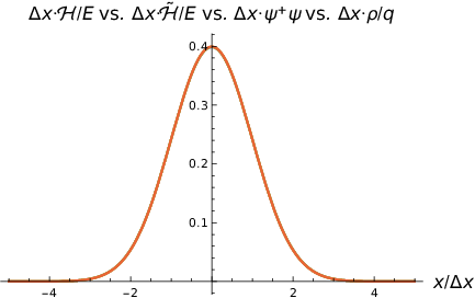
We also note that even in the massless case, all the proxies for position become practically identical for large momentum ℏ​k0≫ℏ/Δ​x\hbar k_{0}\gg\hbar/\Delta x. This is illustrated for k0=10/Δ​xk_{0}=10/\Delta x in Fig. 22. The color coding is in principle the same as in Figs. 12 and 13. However, the differences between the four proxies are at the per mil level for k0=10/Δ​xk_{0}=10/\Delta x.

Refer to caption
Figure 22: The normalized canonical energy density ℋ⁡(x,0)/E\mathcal{H}(x,0)/E (92), the normalized energy pseudo-density ℋ~​(x,0)/E\tilde{\mathcal{H}}(x,0)/E (93), the probability pseudo-density |ψ⁡(x,0)|2|\psi(x,0)|^{2}, and the normalized charge density ρ⁡(x,0)/q\rho(x,0)/q (91) for the massless Klein–Gordon field with Gaussian wave packet (98) and k0=10/Δ​xk_{0}=10/\Delta x. The color coding is in principle the same as in Figs. 12 and 13, but there are only per mil level differences between the proxies for k0=10/Δ​xk_{0}=10/\Delta x.

All proxies for k0​Δ​x>>1k_{0}\Delta x>>1 look like the normalized canonical energy density ℋ⁡(x,t)/E\mathcal{H}(x,t)/E, see Fig. 23 for k0=10/Δ​xk_{0}=10/\Delta x.

Refer to caption
Figure 23: The normalized canonical energy density ℋ⁡(x,t)/E\mathcal{H}(x,t)/E of the massless Klein-Gordon field with Gaussian wave packet (98) and k0=10/Δ​xk_{0}=10/\Delta x.

We can explain this behavior from the asymptotic behavior of the wave packet ψ⁡(x,t)\psi(x,t) and the Klein–Gordon field ϕ⁡(x,t)\phi(x,t) that follow from the wave packet (98). The wave packet

ψ⁡(x,t)\displaystyle\psi(x,t) =\displaystyle= (Δ​x22​π3)1/4​∫d​k​exp⁡[i​k​x−Δ​x2​(k−k0)2−i​c​|k|​t]\displaystyle\left(\frac{\Delta x^{2}}{2\pi^{3}}\right)^{1/4}\int\!dk\,\exp[\mathrm{i}kx-\Delta x^{2}(k-k_{0})^{2}-\mathrm{i}c|k|t] (99)
=\displaystyle= 12​(2​π​Δ​x2)1/4​exp⁡(i​k0​(x−c​t)−(x−c​t)24​Δ​x2)\displaystyle\frac{1}{2(2\pi\Delta x^{2})^{1/4}}\exp\!\left(\mathrm{i}k_{0}(x-ct)-\frac{(x-ct)^{2}}{4\Delta x^{2}}\right)
×[1+erf⁡(Δ​x⋅k0+i​x−c​t2​Δ​x)]\displaystyle\times\left[1+\mathrm{erf}\!\left(\Delta x\cdot k_{0}+\mathrm{i}\frac{x-ct}{2\Delta x}\right)\right]
+12​(2​π​Δ​x2)1/4​exp⁡(i​k0​(x+c​t)−(x+c​t)24​Δ​x2)\displaystyle+\frac{1}{2(2\pi\Delta x^{2})^{1/4}}\exp\!\left(\mathrm{i}k_{0}(x+ct)-\frac{(x+ct)^{2}}{4\Delta x^{2}}\right)
×[1−erf⁡(Δ​x⋅k0+i​x+c​t2​Δ​x)]\displaystyle\times\left[1-\mathrm{erf}\!\left(\Delta x\cdot k_{0}+\mathrm{i}\frac{x+ct}{2\Delta x}\right)\right]

satisfies

ψ⁡(x,t)\displaystyle\psi(x,t) →\displaystyle\to 1(2​π​Δ​x2)1/4​exp⁡(i​k0​(x−t)−(x−c​t)24​Δ​x2)\displaystyle\frac{1}{(2\pi\Delta x^{2})^{1/4}}\exp\!\left(\mathrm{i}k_{0}(x-t)-\frac{(x-ct)^{2}}{4\Delta x^{2}}\right) (100)

for Δ​x⋅k0≫1\Delta x\cdot k_{0}\gg 1. The corresponding Klein–Gordon field (here displayed for k0≥0k_{0}\geq 0)

ϕ⁡(x,t)\displaystyle\phi(x,t) =\displaystyle= (Δ​x28​π3​c2)1/4​∫d​k|k|​exp⁡[i​k​x−Δ​x2​(k−k0)2−i​c​|k|​t]\displaystyle\left(\frac{\Delta x^{2}}{8\pi^{3}c^{2}}\right)^{1/4}\int\!\frac{dk}{\sqrt{|k|}}\,\exp[\mathrm{i}kx-\Delta x^{2}(k-k_{0})^{2}-\mathrm{i}c|k|t]
=\displaystyle= 14​(π2​c2​Δ​x2)1/4​exp⁡(−Δ​x2​k022)​exp⁡(i​k0​x−c​t2−(x−c​t)28​Δ​x2)\displaystyle\frac{1}{4}\left(\frac{\pi}{2c^{2}\Delta x^{2}}\right)^{1/4}\exp\!\left(-\,\frac{\Delta x^{2}k_{0}^{2}}{2}\right)\exp\!\left(\mathrm{i}k_{0}\frac{x-ct}{2}-\frac{(x-ct)^{2}}{8\Delta x^{2}}\right)
×2​Δ​x2​k0+i⁡(x−c​t)[I−14([2​Δ​x2​k0+i⁡(x−c​t)]28​Δ​x2)\displaystyle\times\sqrt{2\Delta x^{2}k_{0}+\mathrm{i}(x-ct)}\left[I_{-\frac{1}{4}}\!\left(\frac{[2\Delta x^{2}k_{0}+\mathrm{i}(x-ct)]^{2}}{8\Delta x^{2}}\right)\right.
+I14([2​Δ​x2​k0+i⁡(x−c​t)]28​Δ​x2)]\displaystyle+\left.I_{\frac{1}{4}}\!\left(\frac{[2\Delta x^{2}k_{0}+\mathrm{i}(x-ct)]^{2}}{8\Delta x^{2}}\right)\right]
+12​(8​π3​c2​Δ​x2)1/4​exp⁡(−Δ​x2​k022)​exp⁡(i​k0​x+c​t2−(x+t)28​Δ​x2)\displaystyle+\frac{1}{2(8\pi^{3}c^{2}\Delta x^{2})^{1/4}}\exp\!\left(-\,\frac{\Delta x^{2}k_{0}^{2}}{2}\right)\exp\!\left(\mathrm{i}k_{0}\frac{x+ct}{2}-\frac{(x+t)^{2}}{8\Delta x^{2}}\right)
×2​Δ​x2​k0+i⁡(x+c​t)​K14​([2​Δ​x2​k0+i⁡(x+c​t)]28​Δ​x2)\displaystyle\times\sqrt{2\Delta x^{2}k_{0}+\mathrm{i}(x+ct)}K_{\frac{1}{4}}\!\left(\frac{[2\Delta x^{2}k_{0}+\mathrm{i}(x+ct)]^{2}}{8\Delta x^{2}}\right)

satisfies

ϕ⁡(x,t)\displaystyle\phi(x,t) →\displaystyle\to (Δ​x2/2​π​c2)1/42​Δ​x2​k0+i⁡(x−c​t)​exp⁡(i​k0​(x−c​t)−(x−c​t)24​Δ​x2)\displaystyle\frac{(\Delta x^{2}/2\pi c^{2})^{1/4}}{\sqrt{2\Delta x^{2}k_{0}+\mathrm{i}(x-ct)}}\exp\!\left(\mathrm{i}k_{0}(x-ct)-\frac{(x-ct)^{2}}{4\Delta x^{2}}\right) (101)

for Δ​x⋅k0≫1\Delta x\cdot k_{0}\gg 1.

As a consequence of (100) and (101), all the proxies for position satisfy

ℋ⁡(x,t)/E\displaystyle\mathcal{H}(x,t)/E →\displaystyle\to ϱ⁡(x,t)/q→ℋ~​(x,t)/E→|ψ⁡(x,t)|2\displaystyle\varrho(x,t)/q\to\tilde{\mathcal{H}}(x,t)/E\to|\psi(x,t)|^{2} (102)
→\displaystyle\to 12​π​Δ​x2​exp⁡(−(x−c​t)22​Δ​x2)\displaystyle\frac{1}{\sqrt{2\pi\Delta x^{2}}}\exp\!\left(-\,\frac{(x-ct)^{2}}{2\Delta x^{2}}\right)

for Δ​x⋅k0≫1\Delta x\cdot k_{0}\gg 1. In spite of the nonlocal relations between the position proxies, they do yield the same results even in the massless limit if Δ​x⋅k0≫1\Delta x\cdot k_{0}\gg 1. We can understand this behavior also directly from Eq. (58), which yields E≃ℏ​ω​(𝒌0)E\simeq\hbar\omega(\bm{k}_{0}) and

ℋ⁡(𝒙,t)/E≃ϱ⁡(𝒙,t)/q≃ℋ~​(𝒙,t)/E≃|ψ⁡(𝒙,t)|2.\mathcal{H}(\bm{x},t)/E\simeq\varrho(\bm{x},t)/q\simeq\tilde{\mathcal{H}}(\bm{x},t)/E\simeq|\psi(\bm{x},t)|^{2}. (103)

8 Applications to Dirac fields

Our results for Klein–Gordon fields have direct impacts for Dirac fields, too. To elucidate this, we recall that the free Dirac field can be written in the form

Ψ⁡(𝒙,t)\displaystyle\Psi(\bm{x},t) =\displaystyle= 12​π3∫d3𝒌∑s[bs(𝒌)u(𝒌,s)exp(ik⋅x)\displaystyle\frac{1}{\sqrt{2\pi}^{3}}\int\!d^{3}\bm{k}\sum_{s}\big[b_{s}(\bm{k})u(\bm{k},s)\exp(\mathrm{i}k\cdot x) (104)
+ds+(𝒌)v(𝒌,s)exp(−ik⋅x)]\displaystyle+d_{s}^{+}(\bm{k})v(\bm{k},s)\exp(-\,\mathrm{i}k\cdot x)\big]

with k⋅x≡𝒌⋅𝒙−ω⁡(𝒌)​tk\cdot x\equiv\bm{k}\cdot\bm{x}-\omega(\bm{k})t and the basis of normalized 4-spinors

u⁡(𝒌,12)\displaystyle u(\bm{k},{\scriptstyle\frac{1}{2}}) =\displaystyle= 12​E​(𝒌)​[E⁡(𝒌)+m​c2]​(E⁡(𝒌)+m​c20ℏ​c​k3ℏ​c​k+),\displaystyle\frac{1}{\sqrt{2E(\bm{k})[E(\bm{k})+mc^{2}]}}\left(\begin{array}[]{c}E(\bm{k})+mc^{2}\\ 0\\ \,\,\hbar ck_{3}\\ \,\,\,\hbar ck_{+}\\ \end{array}\right)\!,
u⁡(𝒌,−12)\displaystyle u(\bm{k},{\scriptstyle-\frac{1}{2}}) =\displaystyle= 12​E​(𝒌)​[E⁡(𝒌)+m​c2]​(0E⁡(𝒌)+m​c2ℏ​c​k−−ℏ​c​k3),\displaystyle\frac{1}{\sqrt{2E(\bm{k})[E(\bm{k})+mc^{2}]}}\left(\begin{array}[]{c}0\\ E(\bm{k})+mc^{2}\\ \,\,\,\hbar ck_{-}\\ \!\!\!\!-\,\hbar ck_{3}\\ \end{array}\right)\!,
v⁡(𝒌,−12)\displaystyle v(\bm{k},{\scriptstyle-\frac{1}{2}}) =\displaystyle= 12​E​(𝒌)​[E⁡(𝒌)+m​c2]​(ℏ​c​k3ℏ​c​k+E⁡(𝒌)+m​c20),\displaystyle\frac{1}{\sqrt{2E(\bm{k})[E(\bm{k})+mc^{2}]}}\left(\begin{array}[]{c}\,\,\hbar ck_{3}\\ \,\,\,\hbar ck_{+}\\ E(\bm{k})+mc^{2}\\ 0\\ \end{array}\right)\!,
v⁡(𝒌,12)\displaystyle v(\bm{k},{\scriptstyle\frac{1}{2}}) =\displaystyle= 12​E​(𝒌)​[E⁡(𝒌)+m​c2]​(ℏ​c​k−−ℏ​c​k30E⁡(𝒌)+m​c2).\displaystyle\frac{1}{\sqrt{2E(\bm{k})[E(\bm{k})+mc^{2}]}}\left(\begin{array}[]{c}\,\,\,\hbar ck_{-}\\ \!\!\!\!-\,\hbar ck_{3}\\ 0\\ E(\bm{k})+mc^{2}\\ \end{array}\right)\!.

Here k±=k1±i​k2k_{\pm}=k_{1}\pm\mathrm{i}k_{2} was used.

In the Dirac case, the 𝒙\bm{x}-space field for a single-particle state

|ψ⁡(t)⟩\displaystyle\bm{|}\psi(t)\bm{\rangle} =\displaystyle= ∑s∫d3​𝒌​bs+​(𝒌)​|0⟩​ψs​(𝒌)​exp⁡(−i​ω𝒌​t),\displaystyle\sum_{s}\int\!d^{3}\bm{k}\,b_{s}^{+}(\bm{k})\bm{|}0\bm{\rangle}\psi_{s}(\bm{k})\exp(-\,\mathrm{i}\omega_{\bm{k}}t), (125)
∑s∫d3​𝒌​|ψs​(𝒌)|2=1,\sum_{s}\int\!d^{3}\bm{k}\,|\psi_{s}(\bm{k})|^{2}=1, (126)

has 4-spinor components

φa​(𝒙,t)\displaystyle\varphi_{a}(\bm{x},t) =\displaystyle= ⟨0|Ψa​(𝒙,t)|ψ⁡(0)⟩=⟨0|Ψa​(𝒙)|ψ⁡(t)⟩\displaystyle\bm{\langle}0\bm{|}\Psi_{a}(\bm{x},t)\bm{|}\psi(0)\bm{\rangle}=\bm{\langle}0\bm{|}\Psi_{a}(\bm{x})\bm{|}\psi(t)\bm{\rangle} (127)
=\displaystyle= 12​π3​∫d3​𝒌​ψs​(𝒌)​ua​(𝒌,s)​exp⁡[i⁡(𝒌⋅𝒙−ω𝒌​t)].\displaystyle\frac{1}{\sqrt{2\pi}^{3}}\int\!d^{3}\bm{k}\,\psi_{s}(\bm{k})u_{a}(\bm{k},s)\exp\!\left[\mathrm{i}(\bm{k}\cdot\bm{x}-\omega_{\bm{k}}t)\right]\!.

We assume a single-particle wave packet,

ψs​(𝒌)=ψ⁡(𝒌)​δs,12.\psi_{s}(\bm{k})=\psi(\bm{k})\delta_{s,\frac{1}{2}}. (128)

The corresponding Fourier transformed wave packet has components ψs​(𝒙,t)=ψ⁡(𝒙,t)​δs,12\psi_{s}(\bm{x},t)=\psi(\bm{x},t)\delta_{s,\frac{1}{2}} with ψ⁡(𝒙,t)\psi(\bm{x},t) given in Eq. (54).

We are focusing on the massless case and spin polarization along the direction of momentum, i.e. k±=0k_{\pm}=0. The 4-spinor (127) then becomes

φ⁡(𝒙,t)=ψ⁡(𝒙,t)​12​(1010).\varphi(\bm{x},t)=\psi(\bm{x},t)\frac{1}{\sqrt{2}}\left(\begin{array}[]{c}1\\ 0\\ 1\\ 0\\ \end{array}\right)\!. (129)

In this case, the normalized charge density coincides with the Born probability density from Fourier transform of the 𝒌\bm{k}-space wave packet,

ϱ⁡(𝒙,t)/q=φ+​(𝒙,t)⋅φ⁡(𝒙,t)=|ψ⁡(𝒙,t)|2,\varrho(\bm{x},t)/q=\varphi^{+}(\bm{x},t)\cdot\varphi(\bm{x},t)=|\psi(\bm{x},t)|^{2}, (130)

while the canonical energy density agrees with the previously defined pseudo-density for energy after taking into account the Dirac equation,

ℋφ\displaystyle\mathcal{H}_{\varphi} =\displaystyle= ℏ​c2​i​(φ+​γ0​𝜸⋅∇φ−∇φ+⋅γ0​𝜸​φ)\displaystyle\frac{\hbar c}{2\mathrm{i}}\left(\varphi^{+}\gamma^{0}\bm{\gamma}\cdot\bm{\nabla}\varphi-\bm{\nabla}\varphi^{+}\cdot\gamma^{0}\bm{\gamma}\varphi\right) (131)
=\displaystyle= i​ℏ2​(ψ+​∂ψ∂t−∂ψ+∂t​ψ)=ℋ~.\displaystyle\frac{\mathrm{i}\hbar}{2}\left(\psi^{+}\frac{\partial\psi}{\partial t}-\frac{\partial\psi^{+}}{\partial t}\psi\right)=\tilde{\mathcal{H}}.

These observations also apply in two spacetime dimensions. A Dirac basis of γ\gamma matrices is provided by

γ0=(− 10     01),γ1=(     01− 10),\gamma_{0}=\left(\begin{array}[]{cc}-\,{1}&{0}\\ \,\,\,\,\,{0}&{1}\\ \end{array}\right)\!,\quad\gamma_{1}=\left(\begin{array}[]{cc}\,\,\,\,\,0&1\\ -\,1&0\\ \end{array}\right)\!, (132)

and the general massless Dirac field is

Ψ⁡(x,t)\displaystyle\Psi({x},t) =\displaystyle= 12​π∫dk[b(k)(11)exp[i(kx−c|k|t)]\displaystyle\frac{1}{2\sqrt{\pi}}\int\!dk\left[b({k})\left(\begin{array}[]{c}1\\ 1\\ \end{array}\right)\exp[\mathrm{i}(kx-c|k|t)]\right.
+d+(k)(     1− 1)exp[−i(kx−c|k|t)]].\displaystyle+\!\left.d^{+}({k})\left(\begin{array}[]{cc}\,\,\,\,\,1\\ -\,1\\ \end{array}\right)\exp[-\,\mathrm{i}(kx-c|k|t)]\right]\!.

The Dirac spinor for the single-particle state

|ψ⁡(t)⟩\displaystyle\bm{|}\psi(t)\bm{\rangle} =\displaystyle= ∫d​𝒌​b+​(k)​|0⟩​ψ​(k)​exp⁡(−i​c​|k|​t),\displaystyle\int\!d\bm{k}\,b^{+}({k})\bm{|}0\bm{\rangle}\psi({k})\exp(-\,\mathrm{i}c|k|t), (139)

is

φ⁡(x,t)=ψ⁡(x,t)​12​(11),\varphi({x},t)=\psi({x},t)\frac{1}{\sqrt{2}}\left(\begin{array}[]{c}1\\ 1\\ \end{array}\right)\!, (140)

and we find again

ϱ⁡(x,t)/q=|ψ⁡(x,t)|2,ℋφ​(x,t)=ℋ~​(x,t).\varrho({x},t)/q=|\psi({x},t)|^{2},\quad\mathcal{H}_{\varphi}({x},t)=\tilde{\mathcal{H}}({x},t). (141)

This means that the canonical energy density of the massless fermion in two spacetime dimensions with initial state (82,139) is now displayed in Figs. 5 and 8, while the normalized charge density now agrees with the Born density displayed in Figs. 6 and 10.

We note in particular that only the Born density is positive definite both for Klein–Gordon fields and for Dirac fields.

9 Conclusions

Even in the single-particle cases, normalized energy density remains the only positive definite position proxy for bosons while normalized charge density remains the only positive definite position proxy for fermions if we insist on expressions in terms of first-quantized fields. On the other hand, Born densities

∑s|ψs​(𝒙,t)|2=1(2​π)3​∑s|∫d3​𝒌​ψs​(𝒌,t)​exp⁡(i​𝒌⋅𝒙)|2\displaystyle\sum_{s}|\psi_{s}(\bm{x},t)|^{2}=\frac{1}{(2\pi)^{3}}\sum_{s}\left|\int\!d^{3}\bm{k}\,\psi_{s}(\bm{k},t)\exp(\mathrm{i}\bm{k}\cdot\bm{x})\right|^{2} (142)

provide positive definite position proxies for any spin by construction, and we have seen that they remain tantalizingly close to the normalized energy and charge densities. The Born densities provide excellent approximations both to normalized energy density and normalized charge density in the limits of low energy (57) or strong localization in 𝒌\bm{k} space (58). However, outside of these limits, the wave packets ψs​(𝒙,t)\psi_{s}(\bm{x},t) are only indirectly related to the corresponding first-quantized fields, and therefore they do not satisfy the corresponding local evolution equations in background fields.

We might consider the Born densities (142) as a common underlying formalism for relativistic particle position. The indirect link of the Born densities to the local dynamics of the corresponding first-quantized fields necessitates position proxies which are directly related to the corresponding first-quantized fields. These position proxies are normalized energy densities for bosons or normalized charge densities for fermions.

Alternatively, we could simply conclude that normalized energy densities are the correct position measures for bosons while normalized charge densities are the correct position measures for fermions, without assumption of a common underlying concept. Our findings cannot rule out this interpretation. However, the assumption of a principal difference in quantum mechanical formalism for bosons and fermions appears no less puzzling than the assumption of Born densities as a common concept that only indirectly links to local dynamics in relativistic regimes with large momentum uncertainty.

Acknowledgments

We acknowledge support from the Natural Sciences and Engineering Research Council of Canada.

References

  • [1] Ling-Dong Kong, Hui Wang, Qing-Yuan Zhao, Jia-Wei Guo, Yang-Hui Huang, Hao Hao, Shi Chen, Xue-Cou Tu, La-Bao Zhang, Xiao-Qing Jia, Lin Kang, Jian Chen, and Pei-Heng Wu, Nat. Photon. (2022) https://doi.org/10.1038/s41566-022-01089-6.
  • [2] R. L. Workman et al. (Particle Data Group), Prog. Theor. Exp. Phys. 2022, 083C01 (2022).
  • [3] W. Greiner, Relativistic Quantum Mechanics (Springer, Berlin, 1990).
  • [4] I. Białynicki-Birula and A. Prystupiuk, Phys. Rev. A 103, 052211 (2021).
  • [5] J. R. Oppenheimer, Phys. Rev. 38, 725 (1931).
  • [6] I. Białynicki-Birula, Acta Phys. Pol. A 86, 97 (1994).
  • [7] J. E. Sipe, Phys. Rev. A 52, 1875 (1995).
  • [8] I. Białynicki-Birula, Photon wave function, in E. Wolf (editor), Progress in Optics XXXVI (Elsevier, Amsterdam, 1996), pp. 245–294.
  • [9] M. O. Scully and M. S. Zubairy, Quantum Optics (Cambridge University Press, Cambridge, 1997).
  • [10] O. Keller, Phys. Rev. A 62, 022111 (2000).
  • [11] O. Keller, Phys. Rep. 411, 1 (2005).
  • [12] B. J. Smith and M. G. Raymer, New J. Phys. 9, 414 (2007).
  • [13] I. Białynicki-Birula and Z. Białynicki-Birula, Phys. Rev. Lett. 108, 140401 (2012).
  • [14] I. Białynicki-Birula and Z. Białynicki-Birula, Phys. Rev. A 86, 022118 (2012).
  • [15] R. Dick, Advanced Quantum Mechanics, 3rd ed. (Springer Nature, Cham, 2020).