跳到论文正文
W Papers独立论文阅读器 arXiv:2304.08392 论文正文 计算阅读时间 · 0%
引用这篇论文根据当前论文元数据生成,正式投稿前建议核对。


License: CC BY 4.0
arXiv:2304.08392v2 [math-ph] 22 May 2023

Tℏ{\color[rgb]{0,0,1}\hbar}ermal Spacetime, Part I:
Relativistic Bohmian Mechanics

Gerald Kaiser Affiliation: www.wavelets.com Email: kaiser@wavelets.com
Abstract

By complexifying Minkowski space ℝ1+d{\,\mathbb{R}}^{1+d}, the proper distance σ⁡(x){\sigma}{(x)} and proper time τ⁡(x)\tau{(x)} extend to the real and imaginary parts σ⁡(z){\sigma}{(z)} and τ⁡(z)\tau{(z)} of the complex length ζ⁡(z)≡−z2\zeta{(z)}\equiv\sqrt{-z^{2}} of z=x−i​yz=x-iy (Fig. 1). For holomorphic positive-energy solutions of the Klein-Gordon equation to exist, yy must belong to the future cone V+V_{+}, thus forming a local arrow of time without the need to invoke statistical physics.

The future tube 𝒯+=ℝ1+d−i​V+{\mathcal{T}}_{+}={\,\mathbb{R}}^{1+d}-iV_{+} acts as an extended phase space for the associated classical particle, the two extra variables being the time x0x_{0} and λ=y2>0\lambda=\sqrt{y^{2}}>0. The evaluation maps ez:ψ↦ψ⁡(z)e_{z}\colon\psi{\,\mapsto\,}\psi{(z)} on the space 𝒦{\mathcal{K}} of holomorphic wave functions define a family of fundamental states, eze_{z} being the quantization of z∈𝒯+z\in{\mathcal{T}}_{+} (Section 3) whose nonrelativistic limit is a Gaussian coherent state at time x0=0x_{0}=0 evolving relativistically to x0≠0x_{0}\neq 0; see Figure 3. A norm is defined in 𝒦{\mathcal{K}} by ‖ψ‖2=∫Γd​γ​(z)​|ψ⁡(z)|2\|\psi\|^{2}=\int_{\Gamma}{\rm d}\gamma{(z)}\,|\psi{(z)}|^{2} where Γ\Gamma and d​γ​(z){\rm d}\gamma{(z)} are covariant forms of classical phase space and Liouville measure, respectively (111). We prove that ‖ψ‖2\|\psi\|^{2} is the total conserved charge of a microlocal probability current jμ​(z)j_{\mu}{(z)}, which implies that ‖ψ‖\|\psi\| is identical to the momentum space norm and |ψ⁡(z)|2|\psi{(z)}|^{2} is a probability density on all phase spaces Γ\Gamma (covariant Born rule). This solves a long-standing problem in Klein-Gordon theory. The fundamental states eze_{z} give resolutions of unity for every Γ\Gamma (132), generalizing those for the non-relativistic coherent states. All of this generalizes to Dirac particles [5, Chapter 5].

A direct connection with thermal physics is established in Theorem 1, where it is shown that the average of an operator AA in a relativistic canonical ensemble at the reciprocal temperature β\beta in a reference frame with its time axis along the unit vector u∈V+u\in V_{+} is an integral of A~​(z−i​ϑ){\tilde{A}}(z-i\vartheta) over z∈Γz\in\Gamma, where A~​(z)=⟨ez|A|ez⟩{\tilde{A}}{(z)}=\langle\,e_{z}|A|e_{z}\,\rangle, ϑ≡12​ℏ​β​u\vartheta\equiv\tfrac{1}{2}\hbar\beta u is the thermal vector specifying a quantum equilibrium frame and its temperature, and Γ\Gamma is any covariant phase space. This proves that the ensemble of the thermal approach is the family of all “hidden” phase-space trajectories of the associated classical particle.

Interactions with gauge fields are included through holomorphic gauge theory (Section 4), which modifies the canonical ensemble by introducing a fiber metric g⁡(z)g{(z)} in the quantum Hilbert space.

For Angela,

With Love & Gratitude

1 A Problem with Minkowski space

Flat spacetime in D=1+dD=1+d dimensions is an affine space equivalent, as a set, to ℝD{{\mathbb{R}\hskip 0.5pt}^{D}}. It is not a vector space because no privileged event exists playing the role of origin. Rather, any two events a,ba,b can be connected by the vector xx called the spacetime interval from aa to bb, which we write as a row vector. The set of all such intervals forms a vector space MM called Minkowski space. We take the coordinates of xx to be xμx_{\mu} (0≤μ≤d)(0\leq\mu\leq d). Its time-space decomposition is

x=(t,𝒙)wheret=x0∈ℝand𝒙=(x1,⋯,xd)∈ℝd.\displaystyle x=(t,{\boldsymbol{x}})\ \ \text{where}\ \ t=x_{0}\in{\,\mathbb{R}}\ \ \text{and}\ \ {\boldsymbol{x}}=(x_{1},\cdots,x_{d})\in{{\mathbb{R}\hskip 0.5pt}^{d}}. (1)

The Minkowski scalar product of two intervals x,y∈Mx,y\in M is given by

x⋅y\displaystyle x\cdot y =x0​y0−𝒙⋅𝒚=∑μ,ν=0dxμ​ημ​ν​yν≡xμ​ημ​ν​yν,\displaystyle=x_{0}y_{0}-{\boldsymbol{x}}\cdot{\boldsymbol{y}}=\sum_{\mu,\nu=0}^{d}x_{\mu}\eta^{\mu\nu}y_{\nu}\equiv x_{\mu}\eta^{\mu\nu}y_{\nu}, (2)

where units have been chosen so that the universal speed of light c=1c=1 and

ημ​ν=diag​(1,−1,−1,⋯,−1)\displaystyle\eta^{\mu\nu}=\text{diag}(1,-1,-1,\cdots,-1) (3)

is the Minkowski pseudo-metric on MM. (We shall reinsert cc in select formulas when it helps with physical interpretation.) The last identity in (2) illustrates Einstein’s summation convention, where identical superscripts and subscripts in each term are automatically summed over their range.

The Lorentz group 𝒢{\mathcal{G}} is the set of all linear maps

Λ:M→M,x↦x​Λ\displaystyle\Lambda\colon M\to M,\ \ x{\,\mapsto\,}x\Lambda (4)

which preserve the scalar product (2), i.e.,

(x​Λ)⋅(y​Λ)=x⋅y∀x,y∈M.\displaystyle(x\Lambda)\cdot(y\Lambda)=x\cdot y\ \ \forall x,y\in M. (5)
Remark 1

The D×DD\times D matrix Λ\Lambda must act to the left on the row vector xx. If a second Lorentz transformation Λ′\Lambda^{\prime} is applied, the combined action is

(x​Λ)​Λ′=x⁡(Λ​Λ′),\displaystyle(x\Lambda)\Lambda^{\prime}=x(\Lambda\Lambda^{\prime}), (6)

so the order of mappings is from left to right, the same as mathematical writing. The convention (4) could thus be called chronological. Had we taken xx to be a column vector, the order of mappings would be anti-chronological:

Λ′​(Λ​x)=(Λ′​Λ)​x.\displaystyle\Lambda^{\prime}(\Lambda x)=(\Lambda^{\prime}\Lambda)x. (7)

This explains our unconventional preference for row vectors and left-acting operators. The same will apply to quantum wave functions and operators. ♣\clubsuit

However, 𝒢{\mathcal{G}} includes space and time inversions. Unless stated otherwise, we confine ourselves to the restricted Lorentz group, which excludes all inversions:

𝒢0={Λ∈𝒢:detΛ=1​and sgn​(x​Λ)0=sgn​x0​∀x∈M}.\displaystyle{\mathcal{G}}_{0}=\{\Lambda\in{\mathcal{G}}\colon\det\Lambda=1\ \text{and ${\,\rm sgn\,}(x\Lambda)_{0}={\,\rm sgn\,}x_{0}\ \forall x\in M$}\}. (8)

The condition detΛ=1\det\Lambda=1 ensures that the overall orientation of MM remains unchanged, while the invariance of sgn​x0{\,\rm sgn\,}x_{0} ensures that the order of time is preserved, hence so is the orientation of space (since detΛ=1\det\Lambda=1).

The Minkowski quadratic form is the mapping Q:M→ℝQ\colon M\to{\,\mathbb{R}} defined by

Q⁡(x)=t2−r2≡x2,wherer=𝒙⋅𝒙=𝒙2≥0.\displaystyle Q{(x)}=t^{2}-r^{2}\equiv x^{2},\ \ \text{where}\ \ \ r=\sqrt{{\boldsymbol{x}}\cdot{\boldsymbol{x}}}=\sqrt{{\boldsymbol{x}}^{2}}\geq 0. (9)

Since QQ is indefinite, MM breaks into the three Lorentz-invariant sectors

Timelike intervals:V={x∈M:x2>0}Lightlike intervals:L={x∈M:x2=0}Spacelike intervals:S={x∈M:x2<0}\begin{split}\text{Timelike intervals:}\ \ V&=\{x\in M\colon x^{2}>0\}\\ \text{Lightlike intervals:}\ \ L&=\{x\in M\colon x^{2}=0\}\\ \text{Spacelike intervals:}\ \ S&=\{x\in M\colon x^{2}<0\}\end{split} (10)

and MM is their disjoint union

M=V∪L∪S.\displaystyle M=V\cup L\cup S. (11)

VV and LL further break into the disjoint unions

V=V+∪V−V±={(t,𝒓):±t>r}L=L+∪L−L±={(t,𝒓):±t=r}\begin{split}&V=V_{+}\cup V_{-}\qquad V_{\pm}=\{(t,{\boldsymbol{r}})\colon\pm t>r\}\\ &L=L_{+}\cup L_{-}\qquad L_{\pm}=\{(t,{\boldsymbol{r}})\colon\pm t=r\}\end{split} (12)

where

V+is the future coneV−is the past coneL+is the future light coneL−is the past light cone.\begin{split}&V_{+}\ \ \text{is the \sl future cone}\ \ \qquad\quad\ V_{-}\ \ \text{is the \sl past cone}\\ &L_{+}\ \ \text{is the \sl future light cone}\ \ \quad L_{-}\ \ \text{is the \sl past light cone}.\end{split} (13)

The physical significance of the decomposition (11) is as follows.

  1. 1.

    Two distinct events {a,b}\{a,b\} can be made simultaneous by a Lorentz transformation if and only if their interval x=b−ax=b-a is spacelike:

    x2<0⟺x​Λ=(0,𝝈)​for some​Λ∈𝒢0, 0≠𝝈∈ℝd\displaystyle x^{2}<0\Longleftrightarrow x\Lambda=(0,{\boldsymbol{{\sigma}}})\ \text{for some}\ \Lambda\in{\mathcal{G}}_{0},\ {\boldsymbol{0}}\neq{\boldsymbol{{\sigma}}}\in{{\mathbb{R}\hskip 0.5pt}^{d}} (14)

    and (5) then gives x2=−𝝈2x^{2}=-{\boldsymbol{{\sigma}}}^{2}. While 𝝈{\boldsymbol{{\sigma}}} is not Lorentz invariant, its lenght is:

    |𝝈|=−x2≡σ⁡(x)>0,x∈S.\displaystyle|{\boldsymbol{{\sigma}}}|=\sqrt{-x^{2}}\equiv{\sigma}{(x)}>0,\ \ x\in S. (15)

    σ⁡(x){\sigma}{(x)} is then the proper distance between the events.

  2. 2.

    Two distinct events can be Lorentz-transformed to the same spatial location if and only if their interval xx is timelike:

    x2>0⟺x​Λ=(τ⁡(x),𝟎)​for some​Λ∈𝒢0,τ⁡(x)≠0,\displaystyle x^{2}>0\Longleftrightarrow x\Lambda=(\tau{(x)},{\boldsymbol{0}})\ \text{for some}\ \Lambda\in{\mathcal{G}}_{0},\ \tau{(x)}\neq 0,

    and (5) then gives x2=τ​(x)2x^{2}=\tau{(x)}^{2} or

    τ⁡(x)=±x2,x∈V.\displaystyle\tau{(x)}=\pm\sqrt{x^{2}},\ x\in V. (16)

    While |τ⁡(x)||\tau{(x)}| is the usual proper time interval between the events, its sign identifies their chronological order if we set sgn​τ​(x)=sgn​t{\,\rm sgn\,}\tau{(x)}={\,\rm sgn\,}t. This leads to the following definition of chronological proper time interval between aa and bb:

    τ⁡(x)=t^​x2,x∈V\displaystyle\tau{(x)}={\hat{t}}\sqrt{x^{2}},\ \ x\in V (17)

    where11 1 The notation t^=t/|t|{\hat{t}}=t/|t| is just a one-dimensional version of the vector notation 𝒓^=𝒓/|𝒓|{\boldsymbol{\hat{r}}}={\boldsymbol{r}}/|{\boldsymbol{r}}|.

    t^≡t|t|=sgn​t,(t2>r2≥0)\displaystyle{\hat{t}}\equiv\frac{t}{|t|}={\,\rm sgn\,}t,\ (t^{2}>r^{2}\geq 0) (18)

    is invariant under all Λ∈𝒢0\Lambda\in{\mathcal{G}}_{0}. τ⁡(x)\tau{(x)} is the chronologically oriented time interval between the events as measured by a clock whose (straight) worldline passes through both in the future direction. Since x2x^{2} does not determine t^{\hat{t}}, neither does it determine τ⁡(x)\tau{(x)}.

  3. 3.

    Any two events can be connected by a light ray if and only if their interval xx is lightlike:

    x2=0⟺x​Λ=(±|𝝈|,𝝈)​for some​Λ∈𝒢0,𝝈∈ℝd.\displaystyle x^{2}=0\Longleftrightarrow x\Lambda=(\pm|{\boldsymbol{{\sigma}}}|,{\boldsymbol{{\sigma}}})\ \text{for some}\ \Lambda\in{\mathcal{G}}_{0},\ {\boldsymbol{{\sigma}}}\in{{\mathbb{R}\hskip 0.5pt}^{d}}. (19)

2 Thermal Spacetime and its Complex Length

Does a single function exist that is defined on all of MM and unifies the proper distance σ⁡(x){\sigma}{(x)} and proper time τ⁡(x)\tau{(x)}? We shall see that it does — but only if we are willing to give up time reversal invariance and allow our spacetime to include all possible arrows of time. The plural arrows is required by Relativity since all future-pointing arrows are equivalent under 𝒢0{\mathcal{G}}_{0}, as are all past-pointing arrows.

An obvious starting point is the observation that

−x2={σ⁡(x)>0,x2<0±i​τ​(x),x2>0\displaystyle\sqrt{-x^{2}}=\begin{cases}{\sigma}{(x)}>0,&x^{2}<0\\ \pm i\tau{(x)},&x^{2}>0\end{cases} (20)

where the sign in the timelike case is indeterminate since x2x^{2} does not distinguish between past and future. We shall make sense of (20) by complexifying xx to

z=x−i​ywithy2>0.\displaystyle z=x-iy\ \ \text{with}\ \ y^{2}>0. (21)

We call the set 𝒯=M−i​V{\mathcal{T}}=M-iV of all such complex intervals the causal tube.

Remark 2

The causal tube is the disjoint union

𝒯=𝒯+∪𝒯−\displaystyle{\mathcal{T}}={\mathcal{T}}_{+}\cup{\mathcal{T}}_{-} (22)

where

𝒯+={x−iy∈ℂD:x∈M,y∈V+}is the Future Tube𝒯−={x−iy∈ℂD:x∈M,y∈V−}is the Past Tube.\begin{split}{\mathcal{T}}_{+}&=\{x-iy\in{{\mathbb{C}\hskip 0.5pt}^{D}}\colon x\in M,\ y\in V_{+}\}\ \ \text{is the \sl Future Tube}\\ {\mathcal{T}}_{-}&=\{x-iy\in{{\mathbb{C}\hskip 0.5pt}^{D}}\colon x\in M,\ y\in V_{-}\}\ \ \text{is the \sl Past Tube}.\end{split} (23)

𝒯+{\mathcal{T}}_{+} and 𝒯−{\mathcal{T}}_{-} play a central role in quantum field theory [7], where they are called the forward and backward tubes. However, no attempt is made there to interpret 𝒯±{\mathcal{T}}_{\pm} physically, as will be done here; see also [5] and [8]. ♣\clubsuit

Definition 1

The complex length of z∈𝒯z\in{\mathcal{T}} is the analytic continuation of σ⁡(x)=−x2{\sigma}{(x)}=\sqrt{-x^{2}} (15) from S⊂MS\subset M to 𝒯{\mathcal{T}} given by

ζ⁡(z)=−z2=y2−x2+2​i​y⋅x.\displaystyle\boxed{\ \zeta(z)=\sqrt{-z^{2}}=\sqrt{y^{2}-x^{2}+2iy\cdot x}.\ } (24)

The extended proper distance and extended chronological proper time in 𝒯{\mathcal{T}} are

σ⁡(z)=Re​ζ​(z)andτ⁡(z)=Im​ζ​(z).\displaystyle{\sigma}{(z)}={\,\rm Re}\ \zeta{(z)}\ \ \text{\rm and}\ \ \tau{(z)}={\,\rm Im}\ \zeta{(z)}. (25)
Remark 3

Note that ζ⁡(z)\zeta{(z)} cannot vanish in 𝒯{\mathcal{T}} since

ζ⁡(z)=0⇒y2=x2andy⋅x=0,\displaystyle\zeta{(z)}=0\ \Rightarrow\ y^{2}=x^{2}\ \ \text{and}\ \ y\cdot x=0,

which is impossible since xx, like yy, is timelike. Furthermore,

y⋅x=0⇒x2<0⇒−z2=y2−x2>0,\displaystyle y\cdot x=0\ \Rightarrow\ x^{2}<0\ \Rightarrow\ -z^{2}=y^{2}-x^{2}>0,

hence −z2-z^{2} belongs to the the right-hand plane ℂ+{\,\mathbb{C}}_{+} and ζ⁡(z)\zeta{(z)} belongs to the cut plane

ℂ∗=ℂ+=ℂ−N\displaystyle{\,\mathbb{C}}_{*}=\sqrt{{\,\mathbb{C}}_{+}}={\,\mathbb{C}}-N

where NN is the negative real axis. In other words, ζ\zeta is the principal branch of −z2\sqrt{-z^{2}}. ♣\clubsuit

Remark 4

The most important role ζ⁡(z)\zeta{(z)} plays is in quantum theory, where it provides a measure of the distance between fundamental quantum states; see Eq. (103). ♣\clubsuit

Remark 5

In Theorem 1 we relate the new variable yy to the thermal vector

ϑ=12​ℏ​β​u\displaystyle\vartheta=\tfrac{1}{2}\hbar\beta u (26)

where β=y2/ℏ\beta=\sqrt{y^{2}}/\hbar is a relativistic analogue of the reciprocal equilibrium temperature in a quantum canonical ensemble and uu is the DD-velocity of the associated equilibrium frame. This will be the basis of the thermal spacetime interpretation of 𝒯{\mathcal{T}}. ♣\clubsuit

Remark 6

The above notion of “equilibrium” for a single relativistic quantum particle is based on the fact that in our formalism, thermal expectations of operators can be represented as ensemble averages where the ensemble is simply the set of all relativistic phase-space trajectories of the associated classical particle (Theorem 1). These are ‘hidden variables’ according to the Copenhagen interpretation; see Remark 21. This may be related to the notion of quantum equilibrium in Bohmian Mechanics and its connection to Born’s rule [1]; see Remark 15. ♣\clubsuit

Proposition 1

The boundary value of ζ\zeta as y→0y\to 0 in 𝒯±{\mathcal{T}}_{\pm} is the distribution

limy→0ζ⁡(x−i​y)=σ⁡(x)​H​(−x2)±i​τ​(x)​H​(x2)\displaystyle\lim_{y\to 0}\zeta(x-iy)={\sigma}{(x)}H(-x^{2})\pm i\tau{(x)}H(x^{2}) (27)

where HH is the Heaviside step function. This resolves the sign ambiguity in (20).

Proof: If y∈V±y\in V_{\pm} and x2<0x^{2}<0, then

limy→0ζ⁡(x−i​y)=limy→0y2−x2+2​i​y⋅x=−x2=σ⁡(x).\displaystyle\lim_{y\to 0}\zeta(x-iy)=\lim_{y\to 0}\sqrt{y^{2}-x^{2}+2iy\cdot x}=\sqrt{-x^{2}}={\sigma}{(x)}.

If x2>0x^{2}>0, let λ=y2\lambda=\sqrt{y^{2}} and use the invariance of ζ\zeta under 𝒢0{\mathcal{G}}_{0} to transform to a rest frame

y=(±λ,𝟎)∈V±andy⋅x=±λ​t.\displaystyle y=(\pm\lambda,{\boldsymbol{0}})\in V_{\pm}\ \ \text{and}\ \ y\cdot x=\pm\lambda t. (28)

Then

limy→0ζ⁡(x−i​y)=limλ→0λ2−x2±2​i​λ​t,=±i​t^​x2=±i​τ​(x).■\displaystyle\lim_{y\to 0}\zeta(x-iy)=\lim_{\lambda\to 0}\sqrt{\lambda^{2}-x^{2}\pm 2i\lambda t},=\pm i{\hat{t}}\sqrt{x^{2}}=\pm i\tau{(x)}.\ \blacksquare (29)

Figure 1 shows plots of σ,τ{\sigma},\tau, and |ζ||\zeta| with D=2,y=(1,0)D=2,y=(1,0) and x=(t,r)∈ℝ2x=(t,r)\in{{\mathbb{R}\hskip 0.5pt}^{2}}, so that

ζ⁡(t,r)=1+r2−t2+2​i​t≡σ⁡(t,r)+i​τ​(t,r).\displaystyle\zeta(t,r)=\sqrt{1+r^{2}-t^{2}+2it}\equiv{\sigma}(t,r)+i\tau(t,r). (30)
Refer to caption
Figure 1: Plots of σ⁡(z){\sigma}{(z)} and τ⁡(z)\tau{(z)} with y=(1,𝟎)y=(1,{\boldsymbol{0}}): (a) σ⁡(t,r){\sigma}(t,r), (b) τ⁡(t,r)\tau(t,r), (c) |ζ⁡(t,r)||\zeta(t,r)|. Figure (d) is a closeup of |ζ⁡(t,r)||\zeta(t,r)| showing the smooth minimum ζ⁡(0,0)=1\zeta(0,0)=1.

The level surfaces of σ⁡(x){\sigma}{(x)} in SS and τ⁡(x)\tau{(x)} in VV are the hyperboloids

Bσ={x∈S:r2−t2=σ2}⊂S,σ>0Wτ={x∈V:t2−r2=τ2}⊂V,τ≠0.\begin{split}B_{\sigma}&=\{x\in S\colon r^{2}-t^{2}={\sigma}^{2}\}\subset S,\ {\sigma}>0\\ W_{\tau}&=\{x\in V\colon t^{2}-r^{2}=\tau^{2}\}\subset V,\ \tau\neq 0.\end{split} (31)
Proposition 2

The level surfaces of σ⁡(z){\sigma}{(z)} and τ⁡(z)\tau{(z)} with y=(λ,𝟎)y=(\lambda,{\boldsymbol{0}}) are the hyperboloids

ℬσ={x∈M:r2σ2−λ2−t2σ2=1}σ>0𝒲τ={x∈M:t2τ2−r2τ2+λ2=1,t^=τ^},τ≠0\begin{split}{\mathcal{B}}_{\sigma}&=\left\{x\in M\colon\frac{r^{2}}{{\sigma}^{2}-\lambda^{2}}-\frac{t^{2}}{{\sigma}^{2}}=1\right\}\ \ {\sigma}>0\\ {\mathcal{W}}_{\tau}&=\left\{x\in M\colon\frac{t^{2}}{\tau^{2}}-\frac{r^{2}}{\tau^{2}+\lambda^{2}}=1,\ {\hat{t}}={\hat{\tau}}\right\},\ \ \tau\neq 0\end{split} (32)

where the condition t^=τ^{\hat{t}}={\hat{\tau}} eliminates the chronologically dissonant half of the two-sheeted hyperboloid. The intersection

Xσ,τ≡ℬσ∩𝒲τ\displaystyle X_{{\sigma},\tau}\equiv{\mathcal{B}}_{\sigma}\cap{\mathcal{W}}_{\tau} (33)

is the level set of the complex distance:

Xσ,τ={z∈𝒯:ζ⁡(z)=σ+i​τ}.\displaystyle X_{{\sigma},\tau}=\{z\in{\mathcal{T}}\colon\zeta{(z)}={\sigma}+i\tau\}. (34)

As expected,

λ→0⇒ℬσ→Bσ​and​𝒯τ→Vτ.\displaystyle\lambda\to 0\ \Rightarrow\ {\mathcal{B}}_{\sigma}\to B_{\sigma}\ \text{and}\ {\mathcal{T}}_{\tau}\to V_{\tau}. (35)

Proof: For z∈𝒯+z\in{\mathcal{T}}_{+}, we can choose y=(λ,𝟎)y=(\lambda,{\boldsymbol{0}}). Then

ζ=λ2−t2+r2+2​i​λ​t=σ+i​τ,\displaystyle\zeta=\sqrt{\lambda^{2}-t^{2}+r^{2}+2i\lambda t}={\sigma}+i\tau,

from which

λ2−t2+r2=σ2−τ2andλ​t=σ​τ\displaystyle\lambda^{2}-t^{2}+r^{2}={\sigma}^{2}-\tau^{2}\ \ \text{and}\ \ \lambda t={\sigma}\tau

hence

λ2​r2\displaystyle\lambda^{2}r^{2} =λ2​(t2+σ2−τ2−λ2)\displaystyle=\lambda^{2}(t^{2}+{\sigma}^{2}-\tau^{2}-\lambda^{2})
=σ2​τ2+λ2​σ2−λ2​τ2−λ4.\displaystyle={\sigma}^{2}\tau^{2}+\lambda^{2}{\sigma}^{2}-\lambda^{2}\tau^{2}-\lambda^{4}.

The right side factorizes, giving

λ2​r2=(σ2−λ2)​(τ2+λ2)λ​t=σ​τ.\displaystyle\lambda^{2}r^{2}=({\sigma}^{2}-\lambda^{2})(\tau^{2}+\lambda^{2})\qquad\lambda t={\sigma}\tau. (36)

This proves that (σ,τ)({\sigma},\tau) carries information equivalent to (t,r)(t,r) in 𝒯+{\mathcal{T}}_{+}. Hence

r2σ2−λ2=τ2λ2+1r2τ2+λ2=σ2λ2−1,\displaystyle\frac{r^{2}}{{\sigma}^{2}-\lambda^{2}}=\frac{\tau^{2}}{\lambda^{2}}+1\qquad\frac{r^{2}}{\tau^{2}+\lambda^{2}}=\frac{{\sigma}^{2}}{\lambda^{2}}-1,

and (32) follows from λ​t=σ​τ\lambda t={\sigma}\tau. ■\blacksquare

Equations (32) and (36) are not Lorentz-invariant because we chose y=(λ,𝟎)y=(\lambda,{\boldsymbol{0}}) from the outset. This is easily remedied.

Definition 2

Given y∈Vy\in V, let

λ=|y|≡y2andy^=y/λ.\displaystyle\lambda=|y|\equiv\sqrt{y^{2}}\ \ \text{and}\ \ {\hat{y}}=y/\lambda. (37)

The invariant local time and radial coordinates relative to yy are

ty​(x)=y^⋅xandry​(x)=ty2−x2.\displaystyle t_{y}{(x)}={\hat{y}}\cdot x\ \ \text{and}\ \ r_{y}{(x)}=\sqrt{t_{y}^{2}-x^{2}}. (38)

Note that

ty2−ry2=x2=t2−r2\displaystyle t_{y}^{2}-r_{y}^{2}=x^{2}=t^{2}-r^{2}

and

y→(±λ,𝟎)∈V±⇒{ty(x)→±t,ry(x)→r}.\displaystyle y\to(\pm\lambda,{\boldsymbol{0}})\in V_{\pm}\ \Rightarrow\ \{t_{y}{(x)}\to\pm t,\ \ r_{y}{(x)}\to r\}.

By choosing any y∈V+y\in V_{+} and substituting tyt_{y} for tt and ryr_{y} for rr, Equations (36) take the invariant form

λ2​ry2=(σ2−λ2)​(τ2+λ2)λ​ty=σ​τ\displaystyle\lambda^{2}r_{y}^{2}=({\sigma}^{2}-\lambda^{2})(\tau^{2}+\lambda^{2})\qquad\lambda t_{y}={\sigma}\tau (39)

relating the local invariants (ty​(x),ry​(x))(t_{y}{(x)},r_{y}{(x)}) to the global invariants (σ⁡(z),τ⁡(z))({\sigma}{(z)},\tau{(z)}).

Remark 7

A different route to complex spacetime was developed in [6]. ♣\clubsuit

3 The Quantization of 𝒯+{\mathcal{T}}_{+}

We conclude that the Klein-Gordon equation does not have a consistent single-particle interpretation and the naive transcription of the trajectory interpretation of nonrelativistic Schrödinger quantum mechanics into this context does not work. – Peter Holland in [3].

Here we resolve this well-known problem by quantizing a Klein-Gordon particle in the future tube 𝒯+{\mathcal{T}}_{+}, interpreted as an extended phase space. In the process we discover that the quantum randomness in this case is due to averaging “observables” over a hidden 22 2 The ensemble is “hidden” because classical trajectories are not an admissible quantum concept. canonical ensemble consisting of all classical phase-space particle trajectories. This amounts to a phase-space formulation of relativistic Bohmian Mechanics.

Remark 8

Simplified Dirac notation. Let ℌ{\mathfrak{H}} be a complex Hilbert space with inner product ⟨f|g⟩\langle\,f|g\,\rangle linear in ff and antilinear in gg.33 3 This convention works well with the left action of operators. Physicists use the opposite convention. If ℌ{\mathfrak{H}} were finite-dimensional, then the inner product of the row vectors f,gf,g could be expressed in matrix form as

⟨f|g⟩=f​g†\displaystyle\langle\,f|g\,\rangle=fg^{\dagger} (40)

where the column vector g†g^{\dagger} is the Hermitian conjugate of gg. This can be extended to infinite dimensions in a mathematically rigorous way [8]. We adapt f​g†fg^{\dagger} as a simplified form of Dirac’s bra-ket notation ⟨f|g⟩\langle\,f|g\,\rangle. ♣\clubsuit

A massive scalar is a single free spinless relativistic particle of mass m>0m>0. A plane wave with energy-momentum p=(E,𝒑)p=(E,{\boldsymbol{p}}) is given by

ϕp(x)=e−ix⋅p/ℏ=e(i​t​E−i​𝒙⋅𝒑)/ℏ,E=m2+𝒑2.\displaystyle\phi_{p}{(x)}=e^{-ix\cdot p/\hbar}=e^{(itE-i{\boldsymbol{x}}\cdot{\boldsymbol{p}})/\hbar},\quad E=\sqrt{m^{2}+{\boldsymbol{p}}^{2}}. (41)

This is the beginning of quantum mechanics. It associates with a particle of energy-momentum pp a wave of frequency k0k_{0} and wave vector 𝒌{\boldsymbol{k}} given by the Planck–Einstein-de Broglie relations

k0=E/ℏ,𝒌=𝒑/ℏ.\displaystyle k_{0}=E/\hbar,\quad{\boldsymbol{k}}={\boldsymbol{p}}/\hbar. (42)

Since the particle is free, pp belongs to the mass shell

Ωm={(E,𝒑):E=m2+𝒑2,𝒑∈ℝd}.\displaystyle\Omega_{m}=\{(E,{\boldsymbol{p}})\colon E=\sqrt{m^{2}+{\boldsymbol{p}}^{2}},\ {\boldsymbol{p}}\in{{\mathbb{R}\hskip 0.5pt}^{d}}\}. (43)

Since all p∈Ωmp\in\Omega_{m} must have equal weight by Einstein’s Relativity Principle and 𝒑{\boldsymbol{p}} varies over ℝd{{\mathbb{R}\hskip 0.5pt}^{d}}, each pp has weight zero. This means that Ωm\Omega_{m} must be treated as a measure space, where the ‘weight’ of a measurable subset A⊂ΩmA\subset\Omega_{m} is its measure

μ⁡(A)=∫Ad​μ​(p).\displaystyle\mu(A)=\int_{A}{\rm d}\mu{(p)}. (44)

For μ⁡(A)\mu{(A)} to be frame-independent, d​μ{\rm d}\mu must be Lorentz-invariant. To find it, note that for general p=(p0,𝒑)∈V+p=(p_{0},{\boldsymbol{p}})\in V_{+} we have p2−m2=p02−E2p^{2}-m^{2}=p_{0}^{2}-E^{2}, hence

δ⁡(p2−m2)​d​p\displaystyle\delta(p^{2}-m^{2}){\rm d}p =δ⁡((p0−E)​(p0+E))​d​p0​d​𝒑=δ⁡(p0−E)​d​p0​d​𝒑2​E,\displaystyle=\delta((p_{0}-E)(p_{0}+E)){\rm d}p_{0}\,{\rm d}{\boldsymbol{p}}=\delta(p_{0}-E)\,{\rm d}p_{0}\,\frac{{\rm d}{\boldsymbol{p}}}{2E}\,,

proving that d​μ{\rm d}\mu is given uniquely, up to a constant factor, by

d​μ​(p)=d​𝒑2​E(p∈Ωm).\displaystyle{\rm d}\mu{(p)}=\frac{{\rm d}{\boldsymbol{p}}}{2E}\quad(p\in\Omega_{m}). (45)

The numerator d​𝒑{\rm d}{\boldsymbol{p}} is the Galilean-invariant Lebesgue measure on the nonrelativistic momentum space ℝd{{\mathbb{R}\hskip 0.5pt}^{d}}, and the denominator 2​E2E accounts for the curvature of the hyperboloid Ωm\Omega_{m}. Momenta 𝒑{\boldsymbol{p}} with large energies E⁡(𝒑)E({\boldsymbol{p}}) count for less in d​μ{\rm d}\mu than they would in d​𝒑{\rm d}{\boldsymbol{p}}, thus making the space of integrable functions larger:

L1​(d​μ)⊃L1​(d​𝒑).\displaystyle L^{1}({\rm d}\mu)\supset L^{1}({\rm d}{\boldsymbol{p}}). (46)
Remark 9

The curvature factor (2​E)−1(2E)^{-1} in d​μ​(p){\rm d}\mu{(p)} breaks the symmetry between the position and momentum representations of nonrelativistic quantum mechanics, on which the canonical commutation relations and the Heisenberg Uncertainty Principle are based. That complicates many aspects of the theory, including the inner product in the position representation (as compared with the momentum representation (53), which is straightforward), the spatial probability interpretation, and even the existence of position operators. This results in the well-known non-existence of a covariant probability interpretation for massive scalar particles in real spacetime, which will be resolved in thermal spacetime; see also [5, Chapter 4]. ♣\clubsuit

The plane wave ϕp​(x)\phi_{p}{(x)} extends to the entire function

ϕp(z)=e−iz⋅p/ℏ=ϕp(x)e−y⋅p/ℏ,z=x−iy∈ℂD\displaystyle\phi_{p}{(z)}=e^{-iz\cdot p/\hbar}=\phi_{p}{(x)}e^{-y\cdot p/\hbar},\ \ z=x-iy\in{{\mathbb{C}\hskip 0.5pt}^{D}} (47)

satisfying the holomorphic Klein-Gordon equation

−□z​ϕp​(z)≡−∂2ϕp​(z)∂zμ​∂zμ=(m​c/ℏ)2​ϕp​(z).\displaystyle-\Box_{z}\phi_{p}{(z)}\equiv-\frac{\partial^{2}\phi_{p}{(z)}}{\partial z^{\mu}\partial z_{\mu}}=(mc/\hbar)^{2}\phi_{p}{(z)}. (48)

But what happens to a general superposition of such plane waves? The question about the compatibility of the complexification M→𝒯+M\to{\mathcal{T}}_{+} with quantum theory thus comes down to studying the behavior of the function

Ry:Ωm→ℝ,Ry(p)=e−y⋅p/ℏ,wherey∈ℝDandp∈Ωm.\displaystyle R_{y}\colon\Omega_{m}\to{\,\mathbb{R}},\quad R_{y}{(p)}=e^{-y\cdot p/\hbar},\ \text{where}\ y\in{{\mathbb{R}\hskip 0.5pt}^{D}}\ \text{and}\ p\in\Omega_{m}. (49)

A general holomorphic solution of (48) with positive energy is a continuous superposition of holomorphic plane waves ϕp​(z)\phi_{p}{(z)} with all possible p∈Ωmp\in\Omega_{m},

ψ⁡(z)=∫Ωmd​μ​(p)​a​(p)​ϕp​(z).\displaystyle\psi{(z)}=\int_{\Omega_{m}}{\rm d}\mu{(p)}\,a{(p)}\phi_{p}{(z)}. (50)

We call ψ⁡(z)\psi{(z)} and a⁡(p)a{(p)} the zz-representation and pp-representation of the quantum state, respectively. The Hilbert space of the pp-representation is

ℋ≡L2(dμ)={a:Ωm→ℂ,∥a∥<∞}\displaystyle{\mathcal{H}}\equiv L^{2}({\rm d}\mu)=\left\{a\colon\Omega_{m}\to{\,\mathbb{C}},\ \|a\|<\infty\right\} (51)

where the norm ‖a‖≥0\|a\|\geq 0 is given by

‖a‖2≡∫Ωmd​μ​(p)​|a⁡(p)|2\displaystyle\|a\|^{2}\equiv\int_{\Omega_{m}}{\rm d}\mu{(p)}\,|a{(p)}|^{2} (52)

with inner product (40)

a1​a2†≡∫Ωmd​μ​(p)​a1​(p)​a2​(p)∗.\displaystyle a_{1}a_{2}^{\dagger}\equiv\int_{\Omega_{m}}{\rm d}\mu{(p)}\,a_{1}{(p)}a_{2}{(p)}^{*}. (53)

The Hilbert space of the zz-representation is

𝒦={ψ(z)=∫Ωmdμ(p)a(p)e−iz⋅p/ℏ:a∈ℋ}\displaystyle{\mathcal{K}}=\{\psi{(z)}=\int_{\Omega_{m}}\!\!{\rm d}\mu{(p)}\,a{(p)}e^{-iz\cdot p/\hbar}\colon a\in{\mathcal{H}}\} (54)

with inner product imported, initially, from ℋ{\mathcal{H}}:

ψ1​ψ2†≡a1​a2†.\displaystyle\psi_{1}\psi_{2}^{\dagger}\equiv a_{1}a_{2}^{\dagger}. (55)

Clearly, zz must be confined to 𝒯+{\mathcal{T}}_{+} for ψ⁡(z)\psi{(z)} to converge when a∈ℋa\in{\mathcal{H}}. In that case, ψ⁡(z)\psi{(z)} is a holomorphic positive-energy solution of the holomorphic Klein-Gordon equation

−□z​ψ​(z)=(m​c/ℏ)2​ψ​(z).\displaystyle-\Box_{z}\psi{(z)}=(mc/\hbar)^{2}\psi{(z)}. (56)

We shall express ψ1​ψ2†\psi_{1}\psi_{2}^{\dagger} as an integral over a relativistic classical phase space Γ⊂𝒯+\Gamma\subset{\mathcal{T}}_{+} of dimension dimℝΓ=2​d\dim_{{\,\mathbb{R}}}\Gamma=2d. This will give a Lorentz-covariant probability interpretation of ψ⁡(z)\psi{(z)} generalizing the Born rule. As noted before, such an interpretation is missing in MM.

To see how ψ⁡(z)\psi{(z)} and a⁡(p)a{(p)} transform under the restricted Lorentz group 𝒢0{\mathcal{G}}_{0},44 4 Here we must confine ourselves to the reduced Lorentz group 𝒢0{\mathcal{G}}_{0} in order to leave 𝒯±{\mathcal{T}}_{\pm} invariant, as is necessary by Proposition 4. we must first explain how zz transforms. The action of 𝒢{\mathcal{G}} on MM extends to ℂD{{\mathbb{C}\hskip 0.5pt}^{D}} by complex linearity, i.e.,

z​Λ≡x​Λ−i​y​Λ,z=x−i​y∈ℂD,Λ∈𝒢.\displaystyle z\Lambda\equiv x\Lambda-iy\Lambda,\quad z=x-iy\in{{\mathbb{C}\hskip 0.5pt}^{D}},\quad\Lambda\in{\mathcal{G}}. (57)

Since 𝒯+{\mathcal{T}}_{+} is not invariant under z↦−zz{\,\mapsto\,}-z, we must confine our analysis to the restricted Lorentz group 𝒢0{\mathcal{G}}_{0}, whose actions on a⁡(p)a{(p)} and ψ⁡(z)\psi{(z)} are given by

a​U​(Λ)​(p)=a⁡(p​Λ)andψ​U​(Λ)​(z)=ψ⁡(z​Λ),\displaystyle aU(\Lambda){(p)}=a(p\Lambda)\quad\text{and}\quad\psi U(\Lambda){(z)}=\psi(z\Lambda), (58)

from which

U⁡(Λ1​Λ2)=U⁡(Λ1)​U​(Λ2)\displaystyle U(\Lambda_{1}\Lambda_{2})=U(\Lambda_{1})U(\Lambda_{2}) (59)

as required of a representation. From the invariance of Ωm\Omega_{m} and d​μ{\rm d}\mu it follows that the pp-representation is unitary, hence so is the zz-representation by (55).

Proposition 3

Reverse Triangle Inequality (Figure (2)).

If yy and pp are any vectors in V+V_{+}, then

y⋅p≥|y|​|p|where|y|=y2and|p|=p2,\displaystyle y\cdot p\geq|y||p|\ \ \text{where}\ \ |y|=\sqrt{y^{2}}\ \ \text{and}\ \ |p|=\sqrt{p^{2}}, (60)

with equality if and only if yy and pp are parallel:

y⋅p=|y|​|p|⟺p^=y^\displaystyle y\cdot p=|y||p|\Longleftrightarrow{\hat{p}}={\hat{y}} (61)

where p^=p/|p|{\hat{p}}=p/|p| and y^=y/|y|{\hat{y}}=y/|y|.

Proof: Choose a ‘rest frame’ with y=(|y|,𝟎)y=(|y|,{\boldsymbol{0}}). Then

y⋅p=|y|​|p|2+𝒑2≥|y|​|p|\displaystyle y\cdot p=|y|\sqrt{|p|^{2}+{\boldsymbol{p}}^{2}}\geq|y||p| (62)

with equality if and only if 𝒑=𝟎{\boldsymbol{p}}={\boldsymbol{0}}, in which case

p=(|p|,𝟎)=|p|​y^⇒y^=p^.\displaystyle p=(|p|,{\boldsymbol{0}})=|p|{\hat{y}}\ \Rightarrow\ {\hat{y}}={\hat{p}}.

By the 𝒢0{\mathcal{G}}_{0}-invariance of y⋅py\cdot p, this is true in any inertial frame. ■\blacksquare

Refer to caption
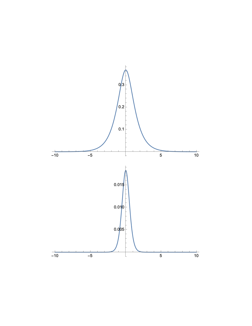
Figure 2: The ray filter (67) in d=1d=1 space dimension with m=ℏ=1,y=(λ,0)m=\hbar=1,\ y=(\lambda,0), and p=(1+q2,q)p=(\sqrt{1+q^{2}},q), thus Sλ​(q)=e−λ​1+q2S_{\lambda}{(q)}=e^{-\lambda\sqrt{1+q^{2}}} in (67). The upper and lower plots show S1​(q)S_{1}{(q)} and S4​(q)S_{4}{(q)}, demonstrating the increasing directivity of RyR_{y} with λ\lambda.
Remark 10

ψ⁡(z)\psi{(z)} as a Relativistic Windowed Fourier Transform.

A Windowed Fourier Transform of f:ℝn→ℂf\colon{{\mathbb{R}\hskip 0.5pt}^{n}}\to{\,\mathbb{C}} has the form

f~​(𝒙,𝒒)=∫ℝnd​𝒌​f^​(𝒌)​ei​𝒙⋅𝒌​W​(𝒌−𝒒),\displaystyle{\tilde{f}}({\boldsymbol{x}},{\boldsymbol{q}})=\int_{{{\mathbb{R}\hskip 0.5pt}^{n}}}{\rm d}{\boldsymbol{k}}\,{\hat{f}}({\boldsymbol{k}})e^{i{\boldsymbol{x}}\cdot{\boldsymbol{k}}}W({\boldsymbol{k}}-{\boldsymbol{q}}), (63)

where f^​(𝒌){\hat{f}}({\boldsymbol{k}}) is the Fourier transform of f⁡(𝒙)f({\boldsymbol{x}}) and W⁡(𝒌)W({\boldsymbol{k}}) is a window centered around the origin. The translates W⁡(𝒌−𝒒)W({\boldsymbol{k}}-{\boldsymbol{q}}) of W⁡(𝒌)W({\boldsymbol{k}}) filter f^{\hat{f}} down to a neighborhood of 𝒒{\boldsymbol{q}} before applying the inverse transform.55 5 The roles of 𝒌{\boldsymbol{k}} and 𝒙{\boldsymbol{x}} can also be interchanged, in which case a spatial window W⁡(𝒙−𝒚)W({\boldsymbol{x}}-{\boldsymbol{y}}) reduces f⁡(𝒙)f({\boldsymbol{x}}) to a neighborhood of 𝒚{\boldsymbol{y}} before computing the Fourier transform. However, (63) is the correct choice in the case (50) since a⁡(p)a{(p)} is in the Fourier domain. See [K11] for a detailed exposition of windowed Fourier transforms, frames, and related matters. Let us compare (63) with (50), written in the form

ψ(x,y)=∫Ωmdμ(p)a(p)e−ix⋅p/ℏRy(p).\displaystyle\psi(x,y)=\int_{\Omega_{m}}{\rm d}\mu{(p)}\,a{(p)}e^{-ix\cdot p/\hbar}R_{y}{(p)}. (64)

If yy is restricted to a single hyperboloid Ωλ⊂𝒯+\Omega_{\lambda}\subset{\mathcal{T}}_{+} (100), then for any y,y′∈Ωλy,y^{\prime}\in\Omega_{\lambda} there exists Λ∈𝒢0\Lambda\in{\mathcal{G}}_{0} such that y′=y​Λy^{\prime}=y\Lambda and any two windows are related by a Lorentz transformation:

Ry′​(p)=Ry​Λ​(p)=Ry​(p​Λ−1).\displaystyle R_{y^{\prime}}{(p)}=R_{y\Lambda}{(p)}=R_{y}(p\Lambda^{-1}). (65)

Thus (64) may be called a Relativistic Windowed Fourier Transform. By comparison, since any two windows W⁡(𝒌−𝒒)W({\boldsymbol{k}}-{\boldsymbol{q}}) and W⁡(𝒌−𝒒′)W({\boldsymbol{k}}-{\boldsymbol{q}}^{\prime}) in (63) are related by a translation, (63) may be called a Euclidean Windowed Fourier Transform. ♣\clubsuit

Proposition 4

For a free massive scalar, the following are true:

  1. 1.

    ψ⁡(z)\psi{(z)} is holomorphic for all a∈ℋa\in{\mathcal{H}} if and only if z∈𝒯z\in{\mathcal{T}} is restricted to 𝒯+{\mathcal{T}}_{+}.

  2. 2.

    Ry​(p)R_{y}{(p)} filters a⁡(p)a{(p)} down to a ray bundle centered around the direction p^=y^{\hat{p}}={\hat{y}}.

  3. 3.

    Ry​(p)R_{y}{(p)} is a ‘bump function’ on Ωm\Omega_{m} peaking at

    py=m​y^.\displaystyle p_{y}=m{\hat{y}}. (66)
  4. 4.

    Ry​(p)R_{y}{(p)} is a guiding filter for the wave ψ⁡(x−i​y)\psi(x-iy), steering it along y^∈V+{\hat{y}}\in V_{+}.

  5. 5.

    λ≡y2\lambda\equiv\sqrt{y^{2}} is a measure of the directivity of RyR_{y}: the greater λ\lambda, the more narrowly the filter is focused around its maximizing direction y^{\hat{y}}.

Thus, all DD components of yy are physically significant.

Proof: If y∈V±y\in V_{\pm}, choose a ‘rest frame’ where y=(±λ,𝟎)y=(\pm\lambda,{\boldsymbol{0}}). Then

Ry​(p)=e∓λ​m2+𝒑2≡S±λ​(𝒑)\displaystyle R_{y}{(p)}=e^{\mp\lambda\sqrt{m^{2}+{\boldsymbol{p}}^{2}}}\equiv S_{\pm\lambda}({\boldsymbol{p}}) (67)

where we have set ℏ=1\hbar=1 for convenience. S−λ​(𝒑)S_{-\lambda}({\boldsymbol{p}}) grows as eλ​|𝒑|e^{\lambda|{\boldsymbol{p}}|}, ruling out y∈V−y\in V_{-}. For y∈V+y\in V_{+}, SλS_{\lambda} decays as e−λ​|𝒑|e^{-\lambda|{\boldsymbol{p}}|} and the integral (50) converges absolutely for all a∈ℋa\in{\mathcal{H}}, defining the function ψ⁡(z)\psi{(z)}. It remains absolutely convergent when differentiated with respect to zμz^{\mu} under the integral sign, so ψ\psi is holomorphic in 𝒯+{\mathcal{T}}_{+}. To prove the other points, choose y=(λ,𝟎)∈V+y=(\lambda,{\boldsymbol{0}})\in V_{+}. Then (67) becomes

Ry​(p)=e−λ​m2+𝒑2≡Sλ​(𝒑),\displaystyle R_{y}{(p)}=e^{-\lambda\sqrt{m^{2}+{\boldsymbol{p}}^{2}}}\equiv S_{\lambda}({\boldsymbol{p}}),

which guides the wave function along a ray bundle centered about p^=y^{\hat{p}}={\hat{y}}. The filter Sλ​(𝒑)S_{\lambda}({\boldsymbol{p}}) becomes exponentially sharper with increasing λ\lambda, as seen in Figure (2). Again, the above proofs are independent of the choice y=(λ,𝟎)y=(\lambda,{\boldsymbol{0}}) due to 𝒢0{\mathcal{G}}_{0}-invariance. ■\blacksquare

Remark 11

Proposition 4 suggests a connection to the de Broglie–Bohm pilot wave theory, [1, 3], but with a fundamental difference:

The pilot is built into the underlying geometry through y∈V+y\in V_{+} and its guiding property follows from the holomorphy of ψ⁡(x−i​y)\psi(x-iy).

Our theory so far is restricted to a single free relativistic particle. The next steps are to

  1. 1.

    extend the theory to NN identical and independent free particles;

  2. 2.

    extend further to N=∞N=\infty and relate this to a free quantum field theory;

  3. 3.

    find a way to include gauge interactions without destroying holomorphy.

These tasks should be guided by the fact that 𝒯+{\mathcal{T}}_{+} is the basis for axiomatic as well as constructive quantum field theory [7, 2]. ♣\clubsuit

Remark 12

While ψ⁡(z)\psi{(z)} is a solution of the Klein-Gordon equation (56), this is not the whole story because it does not explicitly state that it is a positive-energy solution. That fact can be included by requiring that ψ⁡(z)\psi{(z)} be a solution of the psuedo-differential equation

−□z​ψ​(z)=(m​c/ℏ)​ψ​(z),\begin{split}\sqrt{-\Box_{z}}\,\psi{(z)}=(mc/\hbar)\psi{(z)},\end{split} (68)

which is non-local. However, locality can be restored in 𝒯+{\mathcal{T}}_{+} if we replace the positive energy requirement with holomorphy, expressed by the Cauchy-Riemann equations

∂¯μ​ψ​(z)≡∂ψ⁡(z)∂z¯μ=0.\displaystyle{\bar{\partial}}_{\mu}\psi{(z)}\equiv{\frac{\!\partial\psi{(z)}}{\partial{\bar{z}}^{\mu}}}=0. (69)

Then ψ⁡(z)\psi{(z)} is simultaneously a solution of the equations (48) and (69) in 𝒯+{\mathcal{T}}_{+}, both of which are local in 𝒯+{\mathcal{T}}_{+}. Note that the equations remain non-local in MM. ♣\clubsuit

3.1 Review of Nonrelativistic (Gaussian) Coherent States

We shall see that the zz-representation is closely related to nonrelativistic coherent-states representations, which will now be reviewed.

Consider a nonrelativistic particle in ℝd{{\mathbb{R}\hskip 0.5pt}^{d}}, whose position and momentum operators 𝑿,𝑷{\boldsymbol{X}},{\boldsymbol{P}} satisfy the canonical commutation relations

[Xj,Xk]=[Pj,Pk]=0,[Xj,Pk]=i​ℏ​δj​k,1≤j,k≤d\displaystyle[X_{j},X_{k}]=[P_{j},P_{k}]=0,\quad[X_{j},P_{k}]=i\hbar\delta_{jk},\quad 1\leq j,k\leq d (70)

and act on a wave function f⁡(𝒙)∈L2​(ℝd)f({\boldsymbol{x}})\in L^{2}({{\mathbb{R}\hskip 0.5pt}^{d}}) and its Fourier transform f^​(𝒑){\hat{f}}({\boldsymbol{p}}) by

f​Xk​(𝒙)=xk​f​(𝒙)f​Pk​(𝒙)=−i​ℏ​∂f⁡(𝒙)∂xkf^​Xk​(𝒑)=iℏ∂f^​(𝒑)∂pkf^Pk(𝒑)=pkf^(𝒑).\begin{split}fX_{k}({\boldsymbol{x}})&=x_{k}f({\boldsymbol{x}})\qquad\ fP_{k}({\boldsymbol{x}})=-i\hbar{\frac{\!\partial f({\boldsymbol{x}})}{\partial x_{k}}}\\ {\hat{f}}X_{k}({\boldsymbol{p}})&=i\hbar{\frac{\!\partial{\hat{f}}({\boldsymbol{p}})}{\partial p_{k}}}\qquad{\hat{f}}P_{k}({\boldsymbol{p}})=p_{k}{\hat{f}}({\boldsymbol{p}}).\end{split} (71)

To construct coherent states, fix any real number κ\kappa and let

Ak=Xk+i​κ​Pk.\displaystyle A_{k}=X_{k}+i\kappa P_{k}. (72)

Given a normalized state ff, define z∈ℂdz\in{{\mathbb{C}\hskip 0.5pt}^{d}} by

z¯k≡f​Ak​f†=⟨Ak⟩f=⟨Xk⟩f+i​κ​⟨Pk⟩f=x~k+i​κ​p~k.\displaystyle{\bar{z}}_{k}\equiv fA_{k}f^{\dagger}=\langle\,A_{k}\,\rangle_{\!f}=\langle\,X_{k}\,\rangle_{\!f}+i\kappa\langle\,P_{k}\,\rangle_{\!f}={\tilde{x}}_{k}+i\kappa{\tilde{p}}_{k}. (73)

Using the notation

δ​Ak=Ak−⟨Ak⟩f=Ak−z¯k=δ​Xk+i​κ​δ​Pk\displaystyle\delta A_{k}=A_{k}-\langle\,A_{k}\,\rangle_{\!f}=A_{k}-{\bar{z}}_{k}=\delta X_{k}+i\kappa\delta P_{k} (74)

we have ⟨δ​Ak⟩f=0\langle\,\delta A_{k}\,\rangle_{\!f}=0 and

0≤‖f​δ​Ak‖2\displaystyle 0\leq\|f\delta A_{k}\|^{2} =f​δ​Ak​δ​Ak†​f†=⟨Ak​Ak†⟩f−|zk|2\displaystyle=f\delta A_{k}\delta A_{k}^{\dagger}f^{\dagger}=\langle\,A_{k}A_{k}^{\dagger}\,\rangle_{\!f}-|z_{k}|^{2}
=⟨Xk2+κ2​Pk2−i​κ​[Xk,Pk]⟩f−x~k2−κ2​p~k2\displaystyle=\langle\,X_{k}^{2}+\kappa^{2}P_{k}^{2}-i\kappa[X_{k},P_{k}]\,\rangle_{\!f}-{\tilde{x}}_{k}^{2}-\kappa^{2}{\tilde{p}}_{k}^{2}
=(⟨Xk2⟩f−x~k2)+κ2​(⟨Pk2⟩f−p~k2)+ℏ​κ\displaystyle=\left(\langle\,X_{k}^{2}\,\rangle_{\!f}-{\tilde{x}}_{k}^{2}\right)+\kappa^{2}\left(\langle\,P_{k}^{2}\,\rangle_{\!f}-{\tilde{p}}_{k}^{2}\right)+\hbar\kappa
=ΔXk2+κ2​ΔPk2+ℏ​κ\displaystyle=\Delta_{X_{k}}^{2}+\kappa^{2}\Delta_{P_{k}}^{2}+\hbar\kappa

where ΔXk\Delta_{X_{k}} and ΔPk\Delta_{P_{k}} are the usual uncertainties of XkX_{k} and PkP_{k} in the state ff. Since the quadratic form on the right side must be nonnegative for all real κ\kappa, its discriminant must be nonpositive, i.e.,

ℏ2≤4​ΔXk2​ΔPk2\displaystyle\hbar^{2}\leq 4\Delta_{X_{k}}^{2}\Delta_{P_{k}}^{2} (75)

which is the Heisenberg uncertainty principle. Furthermore, equality holds if and only if f​δ​Ak=0f\delta A_{k}=0, so ff is an eigenvector χ𝒛\chi_{\boldsymbol{z}} of AkA_{k} with eigenvalue z¯k{\bar{z}}_{k},

χ𝒛​Ak=z¯k​χ𝒛.\displaystyle\chi_{\boldsymbol{z}}A_{k}={\bar{z}}_{k}\chi_{\boldsymbol{z}}. (76)

The 𝒙{\boldsymbol{x}}-representation (71) of XkX_{k} and PkP_{k} thus gives

xk​χ𝒛​(𝒙)+ℏ​κ​∂χ𝒛​(𝒙)∂xk=z¯k​χ𝒛​(𝒙)\displaystyle x_{k}\chi_{\boldsymbol{z}}({\boldsymbol{x}})+\hbar\kappa\,{\frac{\!\partial\chi_{\boldsymbol{z}}({\boldsymbol{x}})}{\partial x_{k}}}={\bar{z}}_{k}\chi_{\boldsymbol{z}}({\boldsymbol{x}}) (77)

with a unique normalized solution (up to a constant phase factor)

χ𝒛​(𝒙)=N′​exp⁡[(𝒛¯⋅𝒙−𝒙2/2)/ℏ​κ]\displaystyle\chi_{\boldsymbol{z}}({\boldsymbol{x}})=N^{\prime}\exp[({\boldsymbol{\bar{z}}}\cdot{\boldsymbol{x}}-{\boldsymbol{x}}^{2}/2)/\hbar\kappa] (78)

which requires κ>0\kappa>0. Inserting 𝒛¯=𝒙~+i​κ​𝒑~{\boldsymbol{\bar{z}}}={\boldsymbol{\tilde{x}}}+i\kappa{\boldsymbol{\tilde{p}}}, (73) gives

χ𝒛​(𝒙)=N​exp⁡[i​𝒑~⋅𝒙/ℏ−(𝒙−𝒙~)2/2​ℏ​κ]\displaystyle\chi_{\boldsymbol{z}}({\boldsymbol{x}})=N\exp[i{\boldsymbol{\tilde{p}}}\cdot{\boldsymbol{x}}/\hbar-({\boldsymbol{x}}-{\boldsymbol{\tilde{x}}})^{2}/2\hbar\kappa] (79)

with N=N′​exp⁡(𝒙~2/2​ℏ​κ)N=N^{\prime}\exp({\boldsymbol{\tilde{x}}}^{2}/2\hbar\kappa). These are the Gaussian coherent states in the 𝒙{\boldsymbol{x}}-representation.

Similarly, in the 𝒑{\boldsymbol{p}}-representation the Fourier transform χ^𝒛​(𝒑){\hat{\chi}}_{\boldsymbol{z}}({\boldsymbol{p}}) satisfies

i​ℏ​∂χ^𝒛​(𝒑)∂pk+i​κ​pk​χ^𝒛​(𝒑)=z¯k​χ^𝒛​(𝒑)\displaystyle i\hbar{\frac{\!\partial{\hat{\chi}}_{\boldsymbol{z}}({\boldsymbol{p}})}{\partial p_{k}}}+i\kappa p_{k}{\hat{\chi}}_{\boldsymbol{z}}({\boldsymbol{p}})={\bar{z}}_{k}{\hat{\chi}}_{\boldsymbol{z}}({\boldsymbol{p}}) (80)

giving

χ^𝒛​(𝒑)\displaystyle{\hat{\chi}}_{\boldsymbol{z}}({\boldsymbol{p}}) =C′exp[−i𝒛¯⋅𝒑/ℏ−κ𝒑2/2ℏ]=Cexp[−i𝒙~⋅𝒑/ℏ−κ(𝒑−𝒑~)2/2ℏ]\displaystyle=C^{\prime}\exp[-i{\boldsymbol{\bar{z}}}\cdot{\boldsymbol{p}}/\hbar-\kappa{\boldsymbol{p}}^{2}/2\hbar]=C\exp[-i{\boldsymbol{\tilde{x}}}\cdot{\boldsymbol{p}}/\hbar-\kappa({\boldsymbol{p}}-{\boldsymbol{\tilde{p}}})^{2}/2\hbar] (81)

with C=C′​exp⁡(κ​𝒑~2/2​ℏ)C=C^{\prime}\exp(\kappa{\boldsymbol{\tilde{p}}}^{2}/2\hbar). The physical significance of 𝒛=𝒙~−i​κ​𝒚~{\boldsymbol{z}}={\boldsymbol{\tilde{x}}}-i\kappa{\boldsymbol{\tilde{y}}} is that

𝒙~=⟨χ𝒛|𝑿|χ𝒛⟩𝒑~=⟨χ𝒛|𝑷|χ𝒛⟩,\displaystyle{\boldsymbol{\tilde{x}}}=\langle\,\chi_{\boldsymbol{z}}|{\boldsymbol{X}}|\chi_{\boldsymbol{z}}\,\rangle\qquad{\boldsymbol{\tilde{p}}}=\langle\,\chi_{\boldsymbol{z}}|{\boldsymbol{P}}|\chi_{\boldsymbol{z}}\,\rangle, (82)

as required by (73). The uncertainties can be read off from the probability densities:

ρ⁡(𝒙)≡|χ𝒛(𝒙)|2=N2exp[−(𝒙−𝒙~)2/ℏκ]⇒ΔXk=ℏ​κ/2ρ~​(𝒑)≡|χ^𝒛(𝒑)|2=K2exp[−κ(𝒑−𝒑~)2/ℏ]⇒ΔPk=ℏ/2​κ\begin{split}\rho({\boldsymbol{x}})&\equiv|\chi_{\boldsymbol{z}}({\boldsymbol{x}})|^{2}=N^{2}\exp[-({\boldsymbol{x}}-{\boldsymbol{\tilde{x}}})^{2}/\hbar\kappa]\ \Rightarrow\ \Delta_{X_{k}}=\sqrt{\hbar\kappa/2}\\ {\tilde{\rho}}({\boldsymbol{p}})&\equiv|{\hat{\chi}}_{\boldsymbol{z}}({\boldsymbol{p}})|^{2}=K^{2}\exp[-\kappa({\boldsymbol{p}}-{\boldsymbol{\tilde{p}}})^{2}/\hbar]\,\ \Rightarrow\ \Delta_{P_{k}}=\sqrt{\hbar/2\kappa}\end{split} (83)

confirming the minimum-uncertainty property

ΔXk​ΔPk=ℏ/2.\displaystyle\Delta_{X_{k}}\Delta_{P_{k}}=\hbar/2. (84)

3.2 The Fundamental Relativistic Quantum States eze_{z}

The key to understanding the role of zz in quantization is to note that in (50), ψ⁡(z)\psi{(z)} can be expressed as an inner product

ψ⁡(z)=a​ez†whereez​(p)=ϕp​(z)∗=ei​z¯⋅p/ℏ.\displaystyle\psi{(z)}=ae_{z}^{\dagger}\quad\text{where}\quad e_{z}{(p)}=\phi_{p}{(z)}^{*}=e^{i{\bar{z}}\cdot p/\hbar}. (85)

Unlike the plane wave ϕp​(x)\phi_{p}{(x)} (41) in MM, eze_{z} is square-integrable with

∥ez∥2=∫Ωmdμ(p)e−2y⋅p/ℏ=(πmc/λ)νKν(2λmc/ℏ)whereν=d−12\displaystyle\|e_{z}\|^{2}=\int_{\Omega_{m}}{\rm d}\mu{(p)}\,e^{-2y\cdot p/\hbar}=(\pi mc/\lambda)^{\nu}K_{\nu}(2\lambda mc/\hbar)\ \ \ \text{where}\ \ \ \nu=\frac{d-1}{2} (86)

and KνK_{\nu} is the modified Bessel function.

Remark 13

All wavefunctions ψ∈𝒦\psi\in{\mathcal{K}} obey the bound

|ψ⁡(z)|=|a​ez†|≤|a|‖ez‖.♣\displaystyle|\psi{(z)}|=|ae_{z}^{\dagger}|\leq\|a\|\|e_{z}\|.\ \clubsuit (87)

The expectations of the Newton-Wigner position operators XkX_{k} in eze_{z} at t=0t=0 are [5]

⟨Xk⟩ez|t=0≡ez​Xk​ez†ez​ez†=xk,1≤k≤d\displaystyle\langle\,X_{k}\,\rangle_{e_{z}}\big|_{t=0}\equiv\frac{e_{z}X_{k}e_{z}^{\dagger}}{e_{z}e_{z}^{\dagger}}=x_{k}\,,\quad 1\leq k\leq d (88)

and the expectations of the energy-momentum operators PμP_{\mu} in eze_{z} are

⟨Pμ⟩ez≡ez​Pμ​ez†ez​ez†=mλ​c​y^μ0≤μ≤d\displaystyle\langle\,P_{\mu}\,\rangle_{e_{z}}\equiv\frac{e_{z}P_{\mu}e_{z}^{\dagger}}{e_{z}e_{z}^{\dagger}}=m_{\lambda}c\,{\hat{y}}_{\mu}\quad 0\leq\mu\leq d (89)

where

mλ=m​Kν+1​(2​λ​m​c/ℏ)Kν​(2​λ​m​c/ℏ).\displaystyle m_{\lambda}=m\,\frac{K_{\nu+1}(2\lambda mc/\hbar)}{K_{\nu}(2\lambda mc/\hbar)}. (90)
Remark 14

From the definition

Kν​(z)=∫0∞e−z​cosh⁡s​cosh⁡(ν​s)​𝑑s\displaystyle K_{\nu}{(z)}=\int_{0}^{\infty}e^{-z\cosh s}\cosh(\nu s){\rm d}s (91)

it follows that

z>0⇒∂νKν​(z)=∫0∞e−z​cosh⁡s​sinh⁡(ν​s)​s​𝑑s>0∀ν≥0,\displaystyle z>0\ \Rightarrow\ \partial_{\nu}K_{\nu}{(z)}=\int_{0}^{\infty}e^{-z\cosh s}\sinh(\nu s)s\,{\rm d}s>0\ \ \forall\nu\geq 0, (92)

hence by (90),

mλ>m∀λ>0,\displaystyle m_{\lambda}>m\quad\forall\lambda>0, (93)

and the effective mass mλm_{\lambda} of the particle in the (2​d+1)(2d+1)-dimensional state space

𝒯+λ={x−i​y∈𝒯+:y2=λ2}\displaystyle{\mathcal{T}}^{\lambda}_{+}=\{x-iy\in{\mathcal{T}}_{+}\colon y^{2}=\lambda^{2}\} (94)

is greater than its ‘bare’ mass mm. This is a mass renormalization effect due to the convexity of Ωm\Omega_{m} and the fluctuations of the ray filter Ry​(p)R_{y}{(p)} (49) around its maximum value at pyp_{y}. ♣\clubsuit

Proposition 5

The nonrelativistic limit of eze_{z} at t=0t=0 is a Gaussian coherent state.

Proof: Setting c=ℏ=1c=\hbar=1, let

u\displaystyle u =y^=(1+𝒖2,𝒖),𝒖=𝒚/λ\displaystyle={\hat{y}}=(\sqrt{1+{\boldsymbol{u}}^{2}},{\boldsymbol{u}}),\quad{\boldsymbol{u}}={\boldsymbol{y}}/\lambda
v\displaystyle v =p^=(1+𝒗2,𝒗),𝒗=𝒑/m\displaystyle={\hat{p}}=(\sqrt{1+{\boldsymbol{v}}^{2}},{\boldsymbol{v}}),\quad{\boldsymbol{v}}={\boldsymbol{p}}/m

and assume that yy is nonrelativistic, i.e., 𝒖2≪1{\boldsymbol{u}}^{2}\ll 1. By Proposition 4, ez​(p)e_{z}{(p)} is negligible unless pp is also nonrelativistic, i.e., 𝒗2≪1{\boldsymbol{v}}^{2}\ll 1. Then

u≈(1+𝒖2/2,𝒖)v≈(1+𝒗2/2,𝒗)\displaystyle u\approx(1+{\boldsymbol{u}}^{2}/2,{\boldsymbol{u}})\qquad v\approx(1+{\boldsymbol{v}}^{2}/2,{\boldsymbol{v}})

and

u⋅v\displaystyle u\cdot v ≈(1+𝒖2/2)​(1+𝒗2/2)−𝒖⋅𝒗≈1+(𝒖−𝒗)2/2\displaystyle\approx(1+{\boldsymbol{u}}^{2}/2)(1+{\boldsymbol{v}}^{2}/2)-{\boldsymbol{u}}\cdot{\boldsymbol{v}}\approx 1+({\boldsymbol{u}}-{\boldsymbol{v}})^{2}/2
x⋅v\displaystyle x\cdot v =t​1+𝒗2−𝒙⋅𝒗≈t⁡(1+𝒗2/2)−𝒙⋅𝒗\displaystyle=t\sqrt{1+{\boldsymbol{v}}^{2}}-{\boldsymbol{x}}\cdot{\boldsymbol{v}}\approx t(1+{\boldsymbol{v}}^{2}/2)-{\boldsymbol{x}}\cdot{\boldsymbol{v}}

thus

ez​(p)=e−λmu⋅v≈e−λ​mei​x⋅pe−λm(𝒖−𝒗)2/2≈e−λ​m​exp⁡{i​t​(m+𝒑2/2​m)−i​𝒙⋅𝒑−(m​𝒚−λ​𝒑)2/2}.\begin{split}e_{z}{(p)}&=e^{-\lambda mu\cdot v}\approx e^{-\lambda m}e^{ix\cdot p}e^{-\lambda m({\boldsymbol{u}}-{\boldsymbol{v}})^{2}/2}\\ &\approx e^{-\lambda m}\exp\left\{it(m+{\boldsymbol{p}}^{2}/2m)-i{\boldsymbol{x}}\cdot{\boldsymbol{p}}-(m{\boldsymbol{y}}-\lambda{\boldsymbol{p}})^{2}/2\right\}.\end{split} (95)

At t=0t=0, this is a coherent state with expected position and momentum

⟨𝑿⟩z=𝒙,⟨𝑷⟩z=m​𝒚^.\displaystyle\langle\,{\boldsymbol{X}}\,\rangle_{z}={\boldsymbol{x}},\qquad\langle\,{\boldsymbol{P}}\,\rangle_{z}=m{\boldsymbol{\hat{y}}}. (96)

The nonrelativistic free-particle Hamiltonian H=m+𝒑2/2​mH=m+{\boldsymbol{p}}^{2}/2m propagates (95) to time tt, where it no longer has a minimum uncertainty products. This is not surprising since the uncertainty products is not Lorentz invariant. ■\blacksquare

Thus 𝒯+{\mathcal{T}}_{+} can be interpreted as an extended classical phase space for the particle. Since dimℝ𝒯+=2​D\dim_{\,\mathbb{R}}{\mathcal{T}}_{+}=2D and the classical phase space of a single particle in dd space dimensions has dimension 2​d=2​D−22d=2D-2, what are the two extra dimensions in 𝒯+{\mathcal{T}}_{+}? Clearly, one is the time t=x0t=x_{0}. The other is λ\lambda, which may be called the directivity (Proposition 4) or squeezing parameter of the fundamental states eze_{z} (see Figure 3).

Classical phase spaces are thus submanifolds of 𝒯+{\mathcal{T}}_{+} given by specifying tt and λ\lambda. More generally, choose a spacelike submanifold of MM of codimension one, say

Σ={(x∈M:s(x)=0},\displaystyle\Sigma=\{(x\in M\colon s{(x)}=0\}, (97)

whose normal vector nμ​(x)=∂μs⁡(x)n_{\mu}{(x)}=\partial_{\mu}s{(x)} is timelike:66 6 A more careful analysis [5] shows that nn need only be nowhere spacelike, i.e., nμ​(x)​nμ​(x)≥0n_{\mu}{(x)}n^{\mu}{(x)}\geq 0. We shall not explore this option here.

nμ​(x)​nμ​(x)>0.\displaystyle n_{\mu}{(x)}n^{\mu}{(x)}>0. (98)

In general, what we shall call a covariant classical phase space then has the form

Γ≡Γs,λ={x−iy∈𝒯+:s(x)=0,y2=λ2}=Σ−iΩλ\displaystyle\Gamma\equiv\Gamma_{s,\lambda}=\{x-iy\in{\mathcal{T}}_{+}\colon s{(x)}=0,\ y^{2}=\lambda^{2}\}=\Sigma-i\Omega_{\lambda} (99)

where Σ\Sigma is a covariant configuration space and

Ωλ={y∈V+:y2=λ2}\displaystyle\Omega_{\lambda}=\{y\in V_{+}\colon y^{2}=\lambda^{2}\} (100)

is a relativistic momentum space. To complete the picture, we need a symplectic form on Γ\Gamma which must be Lorentz-invariant in order to give invariant inner products in 𝒦{\mathcal{K}}. The cleanest way to do this is to begin with the invariant 2-form [5]

ω=d​xμ∧d​yμ.\displaystyle\omega={\rm d}x_{\mu}\wedge{\rm d}y^{\mu}. (101)

A Lorentz-invariant measure on Γ\Gamma is obtained from the (2​d)(2d)-form

ωd≡ω∧ω∧⋯∧ω=d!​d​xμ^∧d​yμ^\displaystyle\omega^{d}\equiv\omega\wedge\omega\wedge\cdots\wedge\omega=d!\,\widehat{{\rm d}x^{\mu}}\wedge\widehat{{\rm d}y_{\mu}} (102)

where d​xμ^∼d​x/d​xμ\widehat{{\rm d}x^{\mu}}\sim{\rm d}x/{\rm d}x_{\mu} is a dd-form with d​xμ{\rm d}x_{\mu} missing and d​yμ^\widehat{{\rm d}y_{\mu}} is a dd-form with d​yμ{\rm d}y^{\mu} missing [5].

We have seen that the states eze_{z} generalize the Gaussian coherent states. We call them fundamental relativistic quantum states or simply fundamental states because eze_{z} will be seen to be a natural quantization of zz (Remark 18). To see how close they are to being mutually orthogonal, we need the following property from [5, Section 4.4]:

ez​ez′†=(2​π​m​c/ζ)ν​Kν​(m​c​ζ/ℏ),ν=d−12\displaystyle\boxed{\ e_{z}e_{z^{\prime}}^{\dagger}=(2\pi mc/\zeta)^{\nu}K_{\nu}(mc\zeta/\hbar),\ \ \nu=\frac{d-1}{2}\ } (103)

where KνK_{\nu} is a modified Bessel function of the second kind and

ζ≡−w2\displaystyle\zeta\equiv\sqrt{-w^{2}} (104)

is the complex length (24) of the complex interval77 7 The conventions in [5] differ from those used here. Eqs. (86), (90) and (103) reflect the present conventions.

w=z′−z¯=(x′−x)−i⁡(y′+y)∈𝒯+.\displaystyle w=z^{\prime}-{\bar{z}}=(x^{\prime}-x)-i(y^{\prime}+y)\in{\mathcal{T}}_{+}. (105)

Note that when s⁡(x)=x0=ts{(x)}=x_{0}=t, then d​x0=0{\rm d}x_{0}=0 and ωd/d!\omega^{d}/d! reduces to the differential form associated with the usual Liouville measure on the classical phase space:

s⁡(x)=t⇒ωd/d!↦dd​𝒙∧dd​𝒚.\displaystyle s{(x)}=t\ \Rightarrow\ \omega^{d}/d!{\,\mapsto\,}{\rm d}^{d}{\boldsymbol{x}}\wedge{\rm d}^{d}{\boldsymbol{y}}. (106)

Hence we define the relativistic Liouville measure as the (2​d)(2d)-form on 𝒯+{\mathcal{T}}_{+} given by

d​γ​(z)≡N​ωd/d!\displaystyle\boxed{\ {\rm d}\gamma{(z)}\equiv N\omega^{d}/d!\ } (107)

where the normalization constant NN is explained in Proposition 6. Liouville measures covariant with individual phase spaces will be obtained by restricting d​γ​(z){\rm d}\gamma{(z)} to Γ\Gamma.

Definition 3

The inner product in 𝒦{\mathcal{K}} with Γ\Gamma as phase space is

(ψ1​ψ2†)Γ=∫Γd​γ​(z)​ψ1​(z)​ψ2​(z)∗.\displaystyle(\psi_{1}\psi_{2}^{\dagger})_{\Gamma}=\int_{\Gamma}{\rm d}\gamma{(z)}\,\psi_{1}{(z)}\psi_{2}{(z)}^{*}. (108)

By the polarization identity, it suffices to work with the norm

‖ψ‖Γ2=∫Γd​γ​(z)​ρ​(z)whereρ⁡(z)=|ψ⁡(z)|2.\displaystyle\|\psi\|^{2}_{\Gamma}=\int_{\Gamma}{\rm d}\gamma{(z)}\,\rho{(z)}\quad\text{where}\quad\rho{(z)}=|\psi{(z)}|^{2}. (109)
Proposition 6

Let Γ\Gamma be a covariant classical phase space of the form (99). Then for an appropriate choice of NN [5] we have the ‘Plancherel theorem’

‖ψ‖Γ2=‖a‖ℋ2.\displaystyle\|\psi\|^{2}_{\Gamma}=\|a\|^{2}_{{\mathcal{H}}}. (110)

In particular, ‖ψ‖Γ2\|\psi\|^{2}_{\Gamma} is independent of Γ\Gamma and we may write

‖ψ‖2=∫Γd​γ​(z)​|ψ⁡(z)|2∀Γ.\displaystyle\|\psi\|^{2}=\int_{\Gamma}{\rm d}\gamma{(z)}\,|\psi{(z)}|^{2}\quad\forall\ \Gamma. (111)

This was proved in [5], first when Σ\Sigma is a flat time-slice as in (106), i.e.,

‖ψ‖Γ2=N​∫ℝ2​ddd​𝒙​dd​𝒚​ρ​(z).\displaystyle\|\psi\|^{2}_{\Gamma}=N\int_{{\,\mathbb{R}}^{2d}}{\rm d}^{d}{\boldsymbol{x}}\,{\rm d}^{d}{\boldsymbol{y}}\,\rho{(z)}. (112)

The integral on the right is of the Liouville type, given the linear relationship (66) between y^{\hat{y}} and the momentum pyp_{y}. For general Γ\Gamma, we use the fact that the ‘momentum space’ Ωλ\Omega_{\lambda} is a boundary:

Ωλ=−∂BλwhereBλ={y∈V+::y2>λ2}\displaystyle\Omega_{\lambda}=-\partial B_{\lambda}\ \ \text{where}\ \ B_{\lambda}=\{y\in V_{+}\colon:y^{2}>\lambda^{2}\} (113)

where the minus sign indicates the orientation of Ωλ\Omega_{\lambda} toward the convex side of the hyperboloid. The contribution from λ=∞\lambda=\infty vanishes due to the factor e−y⋅p/ℏe^{-y\cdot p/\hbar} in the integrand. Stokes’ theorem then gives

∫Ωλd​yμ^ρ(z)=−∫Bλdy∂ρ⁡(z)∂yμ\displaystyle\int_{\Omega_{\lambda}}\widehat{{\rm d}y_{\mu}}\,\rho{(z)}=-\int_{B_{\lambda}}{\rm d}y\,{\frac{\!\partial\rho{(z)}}{\partial y^{\mu}}} (114)

and so

∥ψ∥2Γ=−N∫Σd​xμ^∫Bλdy∂ρ⁡(z)∂yμ.\displaystyle\|\psi\|^{2}_{\Gamma}=-N\int_{\Sigma}\widehat{{\rm d}x^{\mu}}\int_{B_{\lambda}}{\rm d}y\,{\frac{\!\partial\rho{(z)}}{\partial y^{\mu}}}. (115)

Choose a world volume W⊂MW\subset M bounded by two configuration spaces Σ1,Σ2\Sigma_{1},\Sigma_{2} so that

∂W=Σ2−Σ1\displaystyle\partial W=\Sigma_{2}-\Sigma_{1} (116)

where the corresponding phase spaces (allowing possibly different values of the thermal hyperboloid Ωλ\Omega_{\lambda}) are

Γ1=Σ1−i​Ωλ1Γ2=Σ2−i​Ωλ2\displaystyle\Gamma_{1}=\Sigma_{1}-i\Omega_{\lambda_{1}}\qquad\Gamma_{2}=\Sigma_{2}-i\Omega_{\lambda_{2}} (117)

hence

Γ2−Γ1=∂W−i​∂[Bλ2−Bλ1]=∂[W−i​Ωλ2λ1]\displaystyle\Gamma_{2}-\Gamma_{1}=\partial W-i\partial\left[B_{\lambda_{2}}-B_{\lambda_{1}}\right]=\partial\left[W-i\Omega_{\lambda_{2}}^{\lambda_{1}}\right] (118)

where

Ωλ1λ2=∂[Bλ2−Bλ1]\begin{split}\Omega^{\lambda_{2}}_{\lambda_{1}}=\partial\left[B_{\lambda_{2}}-B_{\lambda_{1}}\right]\end{split} (119)

is a “thickened” phase space with λ1≤λ≤λ2\lambda_{1}\leq\lambda\leq\lambda_{2} (assuming λ1≤λ2\lambda_{1}\leq\lambda_{2}). Thus Γ2\Gamma_{2} is equivalent to Γ1\Gamma_{1} in the sense that their difference is a boundary:

Γ2=Γ1+∂Y\displaystyle\Gamma_{2}=\Gamma_{1}+\partial Y (120)

where YY is the complex world volume

Y=W−i​Ωλ1λ2.\displaystyle Y=W-i\Omega^{\lambda_{2}}_{\lambda_{1}}\,. (121)

A second application of Stokes’ theorem gives

∥ψ∥2Γ2−∥ψ∥2Γ1=−N∫Wdx∫Bλ1λ2dy∂2ρ⁡(z)∂xμ​∂yμ\displaystyle\|\psi\|^{2}_{\Gamma_{2}}-\|\psi\|^{2}_{\Gamma_{1}}=-N\int_{W}{\rm d}x\int_{B^{\lambda_{2}}_{\lambda_{1}}}{\rm d}y\,\frac{\partial^{2}\rho{(z)}}{\partial x_{\mu}\partial y^{\mu}} (122)

where

Bλ1λ2={y∈V+:λ12≤λ2≤λ22}.\displaystyle B^{\lambda_{2}}_{\lambda_{1}}=\{y\in V_{+}\colon\lambda_{1}^{2}\leq\lambda^{2}\leq\lambda_{2}^{2}\}. (123)

Since □z​ρ​(z)=(□z​ψ)​ψ¯=−(m/ℏ)2​ρ​(z)\Box_{z}\rho{(z)}=(\Box_{z}\psi){\bar{\psi}}=-(m/\hbar)^{2}\rho{(z)}, it follows that

∂2ρ⁡(z)∂xμ​∂yμ=i(∂¯μ+∂μ)(∂¯μ−∂μ)ρ(z)=i(□¯z−□z)ρ(z)=0,\begin{split}\frac{\partial^{2}\rho{(z)}}{\partial x_{\mu}\partial y^{\mu}}&=i({\bar{\partial}}^{\mu}+\partial^{\mu})({\bar{\partial}}_{\mu}-\partial_{\mu})\rho{(z)}=i({\bar{\Box}}_{z}-\Box_{z})\rho{(z)}=0,\end{split} (124)

proving that ‖ψ‖Γ2\|\psi\|^{2}_{\Gamma} is independent of Γ\Gamma as claimed. ■\blacksquare

The above proof is not rigorous because it disregards ‘leaks’ that may occur in the integrals (122) at spatial infinity. For a rigorous proof, see [5].

Definition 4

The microlocal current jμ​(z)j_{\mu}{(z)} in 𝒯+{\mathcal{T}}_{+} and the local current Jμ​(x)J_{\mu}{(x)} in MM generated by ρ⁡(z)=|ψ⁡(z)|2\rho{(z)}=|\psi{(z)}|^{2} are given by

jμ​(z)=−N​∂ρ⁡(z)∂yμJμ​(x)≡∫Bλd​y​jμ​(x−i​y).\begin{split}\boxed{\ j_{\mu}{(z)}=-N\,{\frac{\!\partial\rho{(z)}}{\partial y^{\mu}}}\qquad J_{\mu}{(x)}\equiv\int_{B_{\lambda}}{\rm d}y\,j_{\mu}(x-iy).\ }\end{split} (125)

In terms of ψ⁡(z)\psi{(z)},

jμ​(z)=−2​N​Im​(∂μψ⁡(z)⋅ψ​(z)∗)=i​N​ψ​(z)∂μ↔μψ​(z)∗\displaystyle j_{\mu}{(z)}=-2N{\,\rm Im}\ (\partial_{\mu}\psi{(z)}\!\cdot\!\psi{(z)}^{*})=iN\psi{(z)}\stackrel{{\scriptstyle\leftrightarrow}}{{\partial_{\mu}}}\psi{(z)}^{*} (126)

where

ψ1∂μ↔μψ2∗≡(∂μψ1)​ψ2∗−ψ1​∂μψ2∗.\displaystyle\psi_{1}\stackrel{{\scriptstyle\leftrightarrow}}{{\partial_{\mu}}}\psi_{2}^{*}\equiv(\partial_{\mu}\psi_{1})\psi_{2}^{*}-\psi_{1}\partial_{\mu}\psi_{2}^{*}. (127)

By (124), both currents are conserved in MM, i.e., with respect to variations of Σ\Sigma:

∂jμ​(x−i​y)∂xμ=∂Jμ​(x)∂xμ=0.\displaystyle{\frac{\!\partial j_{\mu}(x-iy)}{\partial x_{\mu}}}={\frac{\!\partial J_{\mu}{(x)}}{\partial x_{\mu}}}=0. (128)

This makes

‖ψ‖2=∫Σd​xμ^​Jμ​(x)=∫Σd​xμ^​∫Bλd​y​jμ​(x−i​y)\displaystyle\|\psi\|^{2}=\int_{\Sigma}\widehat{{\rm d}x^{\mu}}\,J_{\mu}{(x)}=\int_{\Sigma}\widehat{{\rm d}x^{\mu}}\int_{B_{\lambda}}{\rm d}y\,j_{\mu}(x-iy) (129)

the total charge of the conserved current Jμ​(x)J_{\mu}{(x)} over Σ\Sigma, as well as that of jμ​(z)j_{\mu}{(z)} over Σ×Bλ\Sigma\times B_{\lambda}. Being conserved, ‖ψ‖2\|\psi\|^{2} is independent of Γ\Gamma, so we can drop the subscript in ‖ψ‖Γ2\|\psi\|^{2}_{\Gamma} .

Remark 15

The fact that the norm

‖ψ‖2=∫Γd​γ​(z)​|ψ⁡(z)|2=‖a‖ℋ2\displaystyle\boxed{\ \|\psi\|^{2}=\int_{\Gamma}{\rm d}\gamma{(z)}\,|\psi{(z)}|^{2}=\|a\|^{2}_{{\mathcal{H}}}\ } (130)

is independent of Γ\Gamma proves that |ψ⁡(z)|2|\psi{(z)}|^{2} is a valid probability density for every covariant phase space. This is a Lorentz-invariant version of the nonrelativistic Born Rule. ♣\clubsuit

Remark 16

Resolution of Unity in terms of the fundamental states: Expressing (130) as

ψ​ψ†=∫Γd​γ​(z)​ψ​ez†​ez​ψ†\displaystyle\psi\psi^{\dagger}=\int_{\Gamma}{\rm d}\gamma{(z)}\,\psi e_{z}^{\dagger}e_{z}\psi^{\dagger} (131)

and peeling away the factors ψ\psi and ψ†\psi^{\dagger} gives the operator equation

∫Γd​γ​(z)​ez†​ez=I\displaystyle\boxed{\ \int_{\Gamma}{\rm d}\gamma{(z)}\,e_{z}^{\dagger}e_{z}=I\ } (132)

for all Γ\Gamma of the form (99), where II is the identity operator on ℋ{\mathcal{H}}. This is a relativistic version of the standard resolution of unity in terms of Gaussian coherent states. ♣\clubsuit

Remark 17

By the Resolution of Unity (132),

ψ⁡(z′)=a​ez′†=∫Γd​γ​(z)​a​ez†​ez​ez′†=∫Γd​γ​(z)​ψ​(z)​K​(z′−z¯).\displaystyle\boxed{\ \psi(z^{\prime})=ae_{z^{\prime}}^{\dagger}=\int_{\Gamma}{\rm d}\gamma{(z)}\,ae_{z}^{\dagger}e_{z}e_{z^{\prime}}^{\dagger}=\int_{\Gamma}{\rm d}\gamma{(z)}\,\psi{(z)}K(z^{\prime}-{\bar{z}}).\ } (133)

If z′∈Γz^{\prime}\in\Gamma, this is a reproducing property generalizing that of the Gaussian coherent states. If z′∉Γz^{\prime}\notin\Gamma, then z′z^{\prime} is either in the future (z′>Γz^{\prime}>\Gamma) or past (z′<Γz^{\prime}<\Gamma) of Γ\Gamma and (133) propagates ψ\psi from Γ\Gamma to z′z^{\prime}. Thus KK unifies the ideas of reproducing kernel and propagator in 𝒦{\mathcal{K}}. Figure 3 shows the behavior of K⁡(z′−z¯)K(z^{\prime}-{\bar{z}}), which measures the correlation between ez′e_{z^{\prime}} and eze_{z}. ♣\clubsuit

Refer to caption
Refer to caption
Figure 3: Plots of the reproducing/propagating kernel KK (133). Top left: Plot of (Re​K​(w))2(\!{\,\rm Re}\ K{(w)})^{2} with d=3d=3 and w=z′−z¯=(t−i​λ,x1,0,0)w=z^{\prime}-{\bar{z}}=(t-i\lambda,x_{1},0,0) Top right: Plot of |K⁡(w)|2|K{(w)}|^{2} with the same parameters Bottom left: Plot of |K⁡(w)|2|K{(w)}|^{2} with λ​m​c=0.1​ℏ\lambda mc=0.1\hbar Bottom right: Plot of |K⁡(w)|2|K{(w)}|^{2} with λ​m​c=20​ℏ\lambda mc=20\hbar. The quadrature complement (Im​K)2(\!{\,\rm Im}\ K)^{2} of (Re​K)2(\!{\,\rm Re}\ K)^{2} has similar oscillations with offset phases, making the sum |K|2|K|^{2} smooth. The level surfaces ℬσ{\mathcal{B}}_{\sigma} and 𝒲τ{\mathcal{W}}_{\tau} (32) give the shape of the beam and its wave fronts, respectively, and λ​m\lambda m controls the directivity of the beam.
Remark 18

Quantization of 𝒯+{\mathcal{T}}_{+}. The mapping

Q:𝒯+→ℋ,z↦ez\displaystyle Q\colon{\mathcal{T}}_{+}\to{\mathcal{H}},\quad z{\,\mapsto\,}e_{z} (134)

sends the (extended) classical state zz to the quantum state eze_{z}, so it may be viewed as a ‘quantization’ of 𝒯+{\mathcal{T}}_{+}. ♣\clubsuit

Remark 19

Fundamental fundamental states for Dirac particles are defined in [5]. ♣\clubsuit

3.3 Bohmian Mechanics of a Single Relativistic Particle

The density matrix of a quantum-mechanical canonical ensemble, representing a system in thermal equilibrium with a heat bath at absolute temperature TT, is88 8 We take Boltzmann’s constant kB=1k_{B}=1, so that TT has units of energy.

ρ=Z−1​e−β​H,β=T−1\displaystyle\rho=Z^{-1}e^{-\beta H},\quad\beta=T^{-1} (135)

where HH is the system’s Hamiltonian operator and

Z=Tr​e−β​H\displaystyle Z={\rm Tr\,}e^{-\beta H} (136)

is the partition function. The thermal expectation value of an operator AA is

⟨A⟩=Tr⁡(A​ρ)=Z−1​Tr​(A​e−β​H).\displaystyle\langle\,A\,\rangle=\mathrm{Tr\,}(A\rho)=Z^{-1}\mathrm{Tr\,}(Ae^{-\beta H}). (137)

Formally, it is possible to build a statistical thermodynamics of a single relativistic particle. For the massive scalar under consideration, the main thermodynamic potentials of the probability distribution ρ⁡(z)\rho{(z)} are:

∙\bullet\ Internal energy U≡⟨H⟩=−Z−1∂βZ=−∂βlnZU\equiv\langle\,H\,\rangle=-Z^{-1}\partial_{\beta}Z=-\partial_{\beta}\ln Z.

∙\bullet\ Entropy S≡−⟨ln⁡ρ⟩=−Tr⁡(ρ​ln⁡ρ)=Φ+β​US\equiv-\langle\,\ln\rho\,\rangle=-\mathrm{Tr\,}(\rho\ln\rho)=\Phi+\beta U where Φ=ln⁡Z\Phi=\ln Z is the Massieu potential.

∙\bullet\ Helmholtz free energy F=U−TS=−Φ/βF=U-TS=-\Phi/\beta.

This begs the question: What is the classical ensemble leading to the above potentials?

Remark 20

The trace of an operator can be computed in the zz-representation by

Tr​B=∫Γd​γ​(z)​B~​(z)whereB~​(z)=ez​B​ez†.\displaystyle\mathrm{Tr\,}B=\int_{\Gamma}{\rm d}\gamma{(z)}\,{\tilde{B}}{(z)}\ \ \text{where}\ \ {\tilde{B}}{(z)}=e_{z}Be_{z}^{\dagger}. (138)

As a partial (and far from rigorous) proof, consider the rank 1 operator ew†​ewe_{w}^{\dagger}e_{w}. By (132),

∫Γd​γ​(z)​ez​ew†​ew​ez†=∫Γd​γ​(z)​ew​ez†​ez​ew†=ew​ew†=Tr⁡(ew†​ew),\displaystyle\int_{\Gamma}{\rm d}\gamma{(z)}\,e_{z}e_{w}^{\dagger}e_{w}e_{z}^{\dagger}=\int_{\Gamma}{\rm d}\gamma{(z)}\,e_{w}e_{z}^{\dagger}e_{z}e_{w}^{\dagger}=e_{w}e_{w}^{\dagger}=\mathrm{Tr\,}(e_{w}^{\dagger}e_{w}), (139)

confirming (138). ♣\clubsuit

Applying (138) to (137) gives

Tr(Ae−β​H)=Tr(e−βH/2Ae−βH/2)=∫Γdγ(z)eze−βH/2Ae−βH/2ez†.\begin{split}\mathrm{Tr\,}(Ae^{-\beta H})=\mathrm{Tr\,}(e^{-\beta H/2}Ae^{-\beta H/2})=\int_{\Gamma}{\rm d}\gamma{(z)}e_{z}e^{-\beta H/2}Ae^{-\beta H/2}e_{z}^{\dagger}.\end{split} (140)

To keep this covariant, choose a unit vector u∈V+u\in V_{+} representing a possible time axis ℝ​u{\,\mathbb{R}}u and let

H=u⋅p,\displaystyle H=u\cdot p, (141)

so that u=(1,𝟎)u=(1,{\boldsymbol{0}}) gives the usual energy. By (85),

eze−βH/2(p)=e(i​z¯−ϑ)⋅p/ℏ=ez−i​ϑ(p)\displaystyle e_{z}e^{-\beta H/2}{(p)}=e^{(i{\bar{z}}-\vartheta)\cdot p/\hbar}=e_{z-i\vartheta}{(p)} (142)

where

ϑ≡12​ℏ​β​u.\displaystyle\vartheta\equiv\tfrac{1}{2}\hbar\beta u. (143)

Since its magnitude |ϑ|=12​ℏ​β|\vartheta|=\tfrac{1}{2}\hbar\beta gives the “equilibrium temperature” and its spacetime direction u=ϑ/|ϑ|u=\vartheta/|\vartheta| gives the “equilibrium frame,” we call ϑ\vartheta the thermal vector.

Theorem 1

The thermal expectation ⟨A⟩\langle\,A\,\rangle can be expressed entirely in terms of integrals over z∈Γz\in\Gamma for any phase space Γ=Σ−i​Ωλ⊂𝒯+\Gamma=\Sigma-i\Omega_{\lambda}\subset{\mathcal{T}}_{+} by

⟨A⟩​(ϑ)=Z~​(ϑ)−1​∫Γd​γ​(z)​A~​(z−i​ϑ)\displaystyle\boxed{\ \langle\,A\,\rangle{(\vartheta)}={\tilde{Z}}{(\vartheta)}^{-1}\int_{\Gamma}{\rm d}\gamma{(z)}\,{\tilde{A}}(z-i\vartheta)\ } (144)

where

A~​(z)=ez​A​ez†andZ~​(ϑ)=∫Γd​γ​(z)​‖ez−i​ϑ‖2.\displaystyle{\tilde{A}}{(z)}=e_{z}Ae_{z}^{\dagger}\ \ \ \text{\rm and}\ \ \ {\tilde{Z}}{(\vartheta)}=\int_{\Gamma}{\rm d}\gamma{(z)}\,\|e_{z-i\vartheta}\|^{2}. (145)

Equation (144) can be expressed in the suggestive form

⟨A⟩​(ϑ)=∫Γd​γ​(z)​ez−i​ϑ​A​ez−i​ϑ†∫Γd​γ​(z)​ez−i​ϑ​ez−i​ϑ†.\displaystyle\langle\,A\,\rangle{(\vartheta)}=\frac{\int_{\Gamma}{\rm d}\gamma{(z)}\,e_{z-i\vartheta}Ae_{z-i\vartheta}^{\dagger}}{\int_{\Gamma}{\rm d}\gamma{(z)}\,e_{z-i\vartheta}e_{z-i\vartheta}^{\dagger}}. (146)

Proof: Assuming the validity of (138), (144) follows from (140) and (142); Z~​(ϑ){\tilde{Z}}{(\vartheta)} is a special case with A=IA=I. ■\blacksquare

Note that the thermal translation

z↦z−i​ϑ=x−i⁡(y+ϑ)\displaystyle z{\,\mapsto\,}z-i\vartheta=x-i(y+\vartheta) (147)

is internal: it leaves xx invariant while dragging yy further away from the origin since

|y+ϑ|=(|y|2+|ϑ|2+2​y⋅ϑ)≥|y|+|ϑ|\displaystyle|y+\vartheta|=\sqrt{\left(|y|^{2}+|\vartheta|^{2}+2y\cdot\vartheta\right)}\geq|y|+|\vartheta| (148)

by (60).

For given ϑ≠0\vartheta\neq 0 (i.e., OPENT<∞)T<\infty), (147) breaks Lorentz symmetry as it selects a preferred equilibrium frame through u∈V+u\in V_{+}. That symmetry is restored if we allow 𝒢0{\mathcal{G}}_{0} to act on the set thermal expectations in all equilibrium frames by

⟨A⟩​U​(Λ)​(ϑ)=⟨A⟩​(ϑ​Λ).\displaystyle\langle\,A\,\rangle U(\Lambda){(\vartheta)}=\langle\,A\,\rangle(\vartheta\Lambda). (149)
Remark 21

Theorem 1 answers the question posed above:

Every phase-space element z∈Γz\in\Gamma in (144) represents a unique classical phase space trajectory of the particle in 𝒯+{\mathcal{T}}_{+}, and the integral ∫Γd​γ​(z)\int_{\Gamma}{\rm d}\gamma{(z)} sums over all such trajectories. The ensemble average is independent of the phase space Γ\Gamma since each Γ\Gamma intersects every classical trajectory exactly once and d​γ​(z){\rm d}\gamma{(z)} is 𝒢0{\mathcal{G}}_{0}-invariant. This proves that ⟨A⟩\langle\,A\,\rangle depends on the trajectories and not their individual points. These trajectories are the microstates of our ensemble.

I hold Remark 21 to be the main result of this investigation. Together with holomorphic gauge theory, which proposes a way to introduce interactions without destroying holomorphy, it gives a solid foundation to relativistic Bohmian mechanics.

Remark 22

For the free particle considered here, the classical trajectories are straight lines. In the next section we propose to include interactions with a gauge field by postulating a fiber metric in the quantum Hilbert space. At the quantum level, the fiber metric subjects the wave function to a gauge interaction. At the classical level, it distorts the trajectories of the associated classical particle to reflect that interaction. ♣\clubsuit

4 Interactions via Holomorphic Gauge Theory

So far we have dealt exclusively with a single free relativistic particle. The requirement that wave functions be holomorphic makes it difficult to introduce interactions through potentials as done in the nonrelativistic theory. We shall instead introduce them covariantly through a method we call Holomorphic Gauge Theory [4]. The probability density ρ⁡(z)=|ψ⁡(z)|2\rho{(z)}=|\psi{(z)}|^{2} and the microlocal current jμ​(z)j_{\mu}{(z)} (125) are invariant under global gauge transformations ψ⁡(z)↦ψ⁡(z)​χ\psi{(z)}{\,\mapsto\,}\psi{(z)}\chi, where χ\chi is constant with |χ|≡1|\chi|\equiv 1. But they are not invariant under microlocal gauge transformations, where χ⁡(z)\chi{(z)} is holomorphic in 𝒯+{\mathcal{T}}_{+} to preserve the holomorphy of ψ\psi, since |χ⁡(z)|≡1|\chi{(z)}|\equiv 1 implies that χ\chi is constant. To admit microlocal gauge transformations, we introduce a fiber metric99 9 Unless gg is constant, it cannot be holomorphic. Still, we write g⁡(z)g{(z)} instead of g⁡(z,z¯)g(z,{\bar{z}}) for brevity. g⁡(z)>0g{(z)}>0 into the Hilbert space 𝒦{\mathcal{K}}, so that the norm (130) becomes

‖ψ‖Γ2=∫Γd​γ​(z)​ρ​(z)\displaystyle\|\psi\|^{2}_{\Gamma}=\int_{\Gamma}{\rm d}\gamma{(z)}\,\rho{(z)} (150)

where

ρ⁡(z)=ψ⁡(z)​g​(z)​ψ​(z)∗\displaystyle\rho{(z)}=\psi{(z)}g{(z)}\psi{(z)}^{*} (151)

is to be interpreted as the particle’s covariant probability density. Then ρ⁡(z)\rho{(z)} is invariant under ψ′​(z)=ψ⁡(z)​χ​(z)\psi^{\prime}{(z)}=\psi{(z)}\chi{(z)} if and only if g⁡(z)g{(z)} absorbs the factor χ⁡(z)\chi{(z)} and its conjugate:

ρ′​(z)=ρ⁡(z)⟺g′​(z)=χ​(z)−1​g​(z)​(χ​(z)∗)−1.\displaystyle\rho^{\prime}{(z)}=\rho{(z)}\ \Longleftrightarrow\ g^{\prime}{(z)}=\chi{(z)}^{-1}g{(z)}(\chi{(z)}^{*})^{-1}. (152)

To find the gauge potential and its curvature field, use the exterior derivative

d=dxμ∂∂xμ+dyμ∂∂yμ=dzμ∂∂zμ+dz¯μ∂∂z¯μ=∂+∂¯\displaystyle{\rm d}={\rm d}x^{\mu}{\frac{\!\partial}{\partial x^{\mu}}}+{\rm d}y^{\mu}{\frac{\!\partial}{\partial y^{\mu}}}={\rm d}z^{\mu}{\frac{\!\partial}{\partial z^{\mu}}}+{\rm d}{\bar{z}}^{\mu}{\frac{\!\partial}{\partial{\bar{z}}^{\mu}}}=\partial+{\bar{\partial}} (153)

where ∂\partial and ∂¯{\bar{\partial}} are the holomorphic and antiholomorphic exterior derivatives, with

d2=0⟺∂2=∂¯2=∂∂¯+∂¯∂=0.\displaystyle{\rm d}^{2}=0\ \Longleftrightarrow\ \partial^{2}={\bar{\partial}}^{2}=\partial{\bar{\partial}}+{\bar{\partial}}\partial=0. (154)

Since ∂ψ​(z)∗=0\partial\psi{(z)}^{*}=0,

∂ρ=∂(ψ​g​ψ∗)\displaystyle\partial\rho=\partial(\psi g\psi^{*}) =∂(ψ​g)​ψ∗=(∂ψ+ψ​∂g⋅g−1)​g​ψ∗=(𝒟​ψ)​g​ψ∗\displaystyle=\partial(\psi g)\psi^{*}=(\partial\psi+\psi\partial g\cdot g^{-1})g\psi^{*}=({\mathcal{D}}\psi)g\psi^{*} (155)

where 𝒟{\mathcal{D}} is the holomorphic exterior derivative

𝒟​ψ​(z)=∂(ψ​g)​g−1=∂ψ+ψ​∂g⋅g−1≡∂ψ+ψ​𝒜\displaystyle{\mathcal{D}}\psi{(z)}=\partial(\psi g)g^{-1}=\partial\psi+\psi\partial g\cdot g^{-1}\equiv\partial\psi+\psi{\mathcal{A}} (156)

with the potential 1-form

𝒜=∂g⋅g−1=∂ln⁡g.\displaystyle{\mathcal{A}}=\partial g\cdot g^{-1}=\partial\ln g. (157)

In the abelian case, the gauge field is given by

ℱ⁡(z)\displaystyle{\mathcal{F}}{(z)} =d​𝒜​(z)=∂¯​𝒜=∂¯​∂ln⁡g⁡(z).\displaystyle={\rm d}{\mathcal{A}}{(z)}={\bar{\partial}}{\mathcal{A}}={\bar{\partial}}\partial\ln g{(z)}. (158)

We have thus arrived at a form of the electromagnetic field as a holomorphic gauge theory for a massive scalar. The potential form 𝒜{\mathcal{A}} is related to the electromagnetic DD-potential 1-form AA by

𝒜⁡(z)=i​A​(z)=(∂μln⁡g⁡(z))​d​zμ.\displaystyle{\mathcal{A}}{(z)}=iA{(z)}=(\partial_{\mu}\ln g{(z)}){\rm d}z^{\mu}. (159)

Thus 𝒜:𝒯+→ℂ{\mathcal{A}}\colon{\mathcal{T}}_{+}\to{\,\mathbb{C}} is derived from a superpotential ln⁡g⁡(z)\ln g{(z)}, something impossible in MM.

The same conservation law (124) making the free norm (130) invariant can now be applied to (151). We find

∂2ρ⁡(z)∂xμ​∂yμ=i(∂¯μ+∂μ)(∂¯μ−∂μ)ρ(z)=i(□¯z−□z)(ψgψ†)=i​ψ​□¯z​(g​ψ†)−i⁡[□z​(ψ​g)]​ψ†=i​ψ​[□z​(ψ​g)]†−i⁡[□z​(ψ​g)]​ψ†.\begin{split}\frac{\partial^{2}\rho{(z)}}{\partial x_{\mu}\partial y^{\mu}}&=i({\bar{\partial}}^{\mu}+\partial^{\mu})({\bar{\partial}}_{\mu}-\partial_{\mu})\rho{(z)}=i({\bar{\Box}}_{z}-\Box_{z})(\psi g\psi^{\dagger})\\ &=i\psi{\bar{\Box}}_{z}(g\psi^{\dagger})-i\left[\Box_{z}(\psi g)\right]\psi^{\dagger}\\ &=i\psi[\Box_{z}(\psi g)]^{\dagger}-i\left[\Box_{z}(\psi g)\right]\psi^{\dagger}.\end{split} (160)

A necessary and sufficient condition for conservation of probability is therefore

−□z​(ψ⁡(z)​g​(z))=ψ⁡(z)​M​(z),whereM⁡(z)=M​(z)∗\displaystyle-\Box_{z}(\psi{(z)}g{(z)})=\psi{(z)}M{(z)},\ \ \text{where}\ \ M{(z)}=M{(z)}^{*} (161)

replaces the factor (m​c/ℏ)2(mc/\hbar)^{2} in (56). M⁡(z)M{(z)} thus plays the role of a mass-squared operator with the gauge-field interactions built in covariantly.

For particles with internal symmetry, the above scalar gauge theory extends to a non-abelian gauge theory where the fiber metric g⁡(z)g{(z)} is a Hermitian n×nn\times n matrix and the gauge potential is given by the matrix-valued 1-form

𝒜=∂g⋅g−1.\displaystyle{\mathcal{A}}=\partial g\cdot g^{-1}. (162)

Since ∂g\partial g need not commute with g−1g^{-1}, 𝒜{\mathcal{A}} cannot generally be expressed in the form ∂ln⁡g\partial\ln g. Hence the non-abelian gauge potential cannot be derived from a superpotential.

The gauge field is given by1010 10 The usual expression for the curvature on a non-abelian gauge field is ℱ=∂¯​𝒜+∂𝒜+𝒜∧𝒜{\mathcal{F}}={\bar{\partial}}{\mathcal{A}}+\partial{\mathcal{A}}+{\mathcal{A}}\wedge{\mathcal{A}}. The sign difference is due to the fact that exterior derivatives act to the right while our operators act to the left.

ℱ=d​𝒜−𝒜∧𝒜=∂¯​𝒜+∂𝒜−𝒜∧𝒜.\displaystyle{\mathcal{F}}={\rm d}{\mathcal{A}}-{\mathcal{A}}\wedge{\mathcal{A}}={\bar{\partial}}{\mathcal{A}}+\partial{\mathcal{A}}-{\mathcal{A}}\wedge{\mathcal{A}}. (163)

However, (162) implies the integrability condition

∂𝒜=−∂g∧∂g−1=∂g∧(g−1∂g⋅g−1)=𝒜∧𝒜,\displaystyle\partial{\mathcal{A}}=-\partial g\wedge\partial g^{-1}=\partial g\wedge(g^{-1}\partial g\cdot g^{-1})={\mathcal{A}}\wedge{\mathcal{A}}, (164)

giving

ℱ=∂¯​𝒜.\displaystyle{\mathcal{F}}={\bar{\partial}}\,{\mathcal{A}}. (165)

The integrability condition thus extends the linear relation between potential and field from the scalar case to the non-abelian case. This – and the superpotential ln⁡g\ln g (157) in the scalar case – gives holomorphic gauge theory a status not shared by ordinary gauge theory.

Remark 23

Holomorphic gauge theory brings gauge theory closer to General Relativity. The former uses a metric defined on the Hilbert space of quantum states while the latter uses a metric on tangent spaces. In the present context, this metric would have the form gμ​ν​(z,z∗)g_{\mu\nu}(z,z^{*}) with zz and z∗z^{*} formally independent, representing a map

gμ​ν:𝒯+×𝒯+∗→ℂ.\displaystyle g_{\mu\nu}\colon{\mathcal{T}}_{+}\times{\mathcal{T}}_{+}^{*}\to{\,\mathbb{C}}. (166)

Just as the Einstein metric is expected to distort free-particle trajectories to follow gravity, so is the fiber metric g⁡(z)g{(z)} expected to distort them to follow the gauge field ℱ{\mathcal{F}}. This will be the subject of future work. ♣\clubsuit

Acknowledgement

I thank Sheldon Goldstein for inspiring me to study Bohmian Mechanics.

References

  • [1] D Dürr, S Goldstein, and N Zanghì, Quantum equilibrium and the origin of absolute uncertainty. J Stat Phys 67, 843–907 (1992). https://doi.org/10.1007/BF01049004
  • [2] J Glimm and A Jaffe, Quantum Physics: A Functional Integral Point of View, 2nd ed. Springer, 1987
  • [3] P R Holland, The Quantum Theory of Motion. Cambridge University Press, 1993
  • [4] G Kaiser, Phase-space approach to relativistic quantum mechanics. III. Quantization, relativity, localization and gauge freedom. J. Math. Phys. 22, 705 (1981). https://doi.org/10.1063/1.524962
  • [5] G Kaiser, Quantum Physics, Relativity, and Complex Spacetime: Towards a New Synthesis. North Holland, 1990. https://arxiv.org/abs/0910.0352
  • [6] G Kaiser, Complex-distance potential theory and hyperbolic equations, in Clifford Analysis, J. Ryan and W. Sprössig, eds., Birkhäuser, Boston, 2000. https://arxiv.org/abs/math-ph/9908031
  • [7] R F Streater and A S Wightman, PCT, Spin and Statistics, and All That. Princeton University Press, 2001
  • [8] G Kaiser, A Friendly Guide to Wavelets. Modern Birkhäuser Classics, Boston, 2011