On poroelastic strain energy degradation in the variational phase–field models for hydraulic fracture
Abstract
Though a number of formulations have been proposed for phase–field models for hydraulic fracture, the definition of the degraded poroelastic strain energy varies from one model to another. This study explores previously proposed forms of the poroelastic strain energy with diffused fracture and assesses their ability to recover the explicit fracture opening aperture. We then propose a new form of degraded poroelastic strain energy derived from micromechanical analyses. Unlike the previously proposed models, our poroelastic strain energy degradation depends not only on the phase–field variable (damage) but also on the type of strain energy decomposition. Comparisons against closed form solutions suggest that our proposed model can recover crack opening displacement more accurately irrespective of Biot’s coefficient or the pore–pressure distribution. We then verify our model against the plane strain hydraulic fracture propagation, known as the KGD fracture, in the toughness dominated regime. Finally, we demonstrate the model’s ability to handle complex hydraulic fracture interactions with a pre–existing natural fracture.
Keywords:
Phase–field; Hydraulic fracture; Multi–scale analysis; Poroelasticity; Fixed stress split1 Introduction
The phase–field model for fracture has become a standard method to simulate fracturing. The model was originally proposed by Bourdin et al. (2000) [12] as a numerical regularization of the variational approach to fracture [39], and can be regarded as a special case for the gradient damage model [77, 62, 30]. Its applications range from ductile [3, 55, 1, 101], dynamic [14, 9, 60, 76], fatigue [83, 20, 52], dessication [65, 19, 47, 63], and to environment assisted fracturing [64, 82, 28, 93, 94, 78]. For hydraulic fracture, which is the main focus of this paper, Bourdin et al. (2012) [11] adapted the phase–field model by including the effects of fluid pressure within fracture and verified the fracture propagation behaviors in an impermeable elastic medium with injection of inviscid fluid. Wheeler et al. (2014) [89] extended the phase–field approach to porous media but with an invariant pore–pressure field, and it was further extended for variant pore–pressure by Mikelić et al.(2015a, 2015b) [70, 71]. Since these pioneering works, many phase–field models for hydraulic fracturing have been proposed. Amongst these models, the differences amount mainly to how to treat these two points: 1) distinct hydraulic responses in reservoir (porous media) and fracture (open channel), and 2) degradation of the poroelastic strain energy. We briefly review these two points in the following.
For two distinct hydraulic responses, various ways to delineate the fracture from the reservoir domain have been proposed. Mikelić et al. (2015a, 2015b) [70, 71] applied a Darcy flow in reservoir and a Poiseuille flow in fracture and relied on the phase–field value to transition between them. Another way to delineate the fracture was proposed by Wilson and Landis (2016) [91] who scaled the fluid viscosity to recover Poiseuille flow in fracture. Santillàn et al. (2017, 2018) [79, 80] also delineated the fracture domain from the reservoir domain based on the phase–field value, but in their approach, the fracture domain is extracted and built separately with one–dimensional line elements to form a hybrid system with two–dimensional reservoir elements. This one–dimensional fracture domain then has to be updated dynamically as the phase–field profile evolves. Another hybrid method was proposed by [26]. They applied the phase–field model for fracture propagation and once fractures fully develop, then the fractured domain is treated with the discrete contact model. Instead of delineating the fracture domain, Miehe et al. (2015) [69] enhanced the permeability as a function of the deformation. Similarly, Yoshioka and Bourdin (2016) [102] enhanced the permeability with a simple threshold based on the phase–field variable. On the other hand, Lee et al. (2017) [57] set a level–set function to average the two flow systems, which has been followed by many studies [107, 58, 111, 90, 61, 59, 97, 110]. Alternatively, Chukwudozie et al. (2019) [24] averaged the flow in fracture domain using phase–field calculus. In [46, 35], the theory of porous media was used instead to transition between the reservoir flow (Darcy) and the fracture flow (Navier–Stokes). Despite all the different ways to treat the two distinct flows (porous medium and fracture), the models appear to generate reasonable fluid pressure responses at least in the toughness dominated hydraulic fracture where the pressure drop within the fracture is negligible [32].
For degradation of the poroelastic strain energy, we have yet seen a convergence while the degradation of the elastic strain energy is more or less standardized. For an elastic medium, the strain energy density without fracture or damage is:
where denotes the elastic tensor, and is the linearlized strain defined as with being the gradient of and being the transpose of . With the phase–field variable , which varies from intact to fully broken , the general degraded strain energy takes the form:
where in the original model [12]. However, other forms of have been proposed depending on the degradation function [92, 95, 81], the type of strain energy decomposition [4, 69, 41, 31], and the material constitutive relationship [75, 87, 112]. For poroelastic media, on the other hand, the so called effective stress, which is the part of the stress borne by the solid, is given as and the total stress, which is balanced with the body force and external loadings, is by where is Biot’s coefficient and is the fluid pressure. While the effective stress (solid part) is degraded with , degradation for the fluid pressure has not arrived at a consensus within the community. Some models do not degrade the fluid pressure at all [48, 108] and some do but in various ways [72, 102, 79, 57]11 1 For desiccation crack in partially saturated porous media, we refer to comprehensive stability analyses by [63]..
Our objective in this study is to derive a poroelastic strain energy that is consistent with the explicit fracture representation where the fluid pressure is localized within the fracture. In other words, the poroelastic deformation from the phase–field model should converge to the one from the explicit fracture as the regularization length scale parameter approaches 0. We first revisit the previously proposed forms of poroelastic strain energy and point out the differences in terms of degradation of the fluid pressure related terms. We then derive a degraded poroelastic strain energy from micromechanical analyses. As it turns out, Biot’s parameters depend not only on the phase–field variable (damage) but also on the type of strain energy decomposition. Our proposed poroelastic strain energy is verified to reproduce the theoretical fracture aperture openings. On the other hand, the previously proposed models require the fluid pressure in fracture to be diffused beyond fully fractured domain or certain value of Biot’s coefficient.
This paper is structured as follows. The next section recalls three existing formulations of poroelastic strain energy in the phase–field model for hydraulic fracture. We then propose a model with phase–field dependent Biot’s parameters and porosity via micromechanical analysis. Section 3 deals with the numerical implementation of the new proposed model in which the fixed stress split strategy is derived for solving the hydro–mechanical phase–field coupling problem. In section 4, the proposed model is verified against the analytical solutions. The accuracy of the four involved formulations in estimating the fracture aperture is highlighted. Section 5 studies interactions between hydraulic fracture and natural fracture. The paper ends with a conclusion and possible future works.
Throughout the paper, the following notations are used. Tensorial product of any second–order tensors and and fourth–order tensor are and . The symbol is used to calculate the norm of any second–order tensor . The identity tensors for the second and fourth order are denoted by and , respectively. The fourth order projector and are expressed in the component form as and , respectively. The trace operator is defined as . is the gradient of , is the transpose of , and is the symmetric part of the gradient of defined as . The overhead dot symbol indicates the time differentiation of variable .
2 Model formulation
In this section, we start with the now established phase–field model by introducing a total energy of an elastic medium. The total energy is composed of the strain energy and the surface energy, and the strain energy needs to be adjusted when applied to poroelastic medium. To explore the required adjustment, we present a three–scale (macro–, meso–, and micro–) poroelastic medium. To clarify, we use “meso–" to indicate an object or quantity at the mesoscale, and “micro–" at the microscale. Two–level homogenization will be presented first to derive the poroelastic behavior, considering meso–cracks and micro–pores. Following that, the phase–field dependent Biot’s parameters and porosity will be introduced to account for macroscale fracture. In this study, we deal with the hydraulic fracture problem in fluid–saturated porous media.
2.1 Phase–field model for fracture
Consider an elastic body embedded with a lower–dimensional macroscopic fracture which is regularized by the well–known phase–field method into (Fig. 1 a). The body is subjected to a surface force on boundary and a flux on . In addition, and are the prescribed pressure and displacement on boundary and , respectively.

The phase–field model is based on the variational approach to fracture proposed by Francfort and Marigo [39] and they defined the total energy of the system (Fig. 1) as a sum of the strain energy and the surface energy:
| (1) |
where is the strain energy density and is the fracture surface energy density. Bourdin et al. [12] proposed to regularize this energy functional following [74] by introducing a phase–field variable 22 2 In this study, we follow the original definition of the phase–field variable where represents fracture and intact material [12]. Thus, corresponds to the degree of damage in the context of damage mechanics. and a regularization length parameter as
| (2) |
where is given as in [12] and is the normalizing parameter given by [66, 85]. The regularized model is referred as AT1 for and as AT2 for [77, 15].
2.2 Extension to poroelastic media
When the phase–field model is applied for a poroelastic medium, we need to account for poroelastic effects in the total energy functional . We consider a poroelastic medium () that consists of a porous matrix () and a crack set () (Fig. 1). Then, we wish to find the regularized effective total energy functional for the poroelastic medium, which can be written as
| (3) |
where is the poroelastic strain energy. Several variations of have been proposed previously and we explore them in the following.
We start with the linear momentum balance and mechanical boundaries of the poroelastic medium in a discrete setting depicted in Fig. 1 (left):
| (4) |
where denotes the Cauchy (total) stress, the body force and the normal vector to the fracture. Let the elasticity stiffness tensor for the poroelastic medium be where and are the bulk modulus and the shear modulus for the porous matrix respectively. Following Biot’s poroelasticity [7], the total stress in the porous matrix () is given as
| (5) |
Let us neglect the body force and the traction in the comparisons that follow in this section for the sake of simplicity. Multiplying (4)-1 by a test function and using Green’s formula, (4)–2 and (4)–3, we have
| (6) |
where denotes a jump quantity over . In [102, 24], they considered the poroelastic strain energy of:
| (7) |
so that (6) is the first variation of (7) with respect to assuming that is a function of . Using a -convergence property and the co-area formula [11, 24], the last term of (7) can be approximated as
Then the regularized poroelastic strain energy can be
| (8) |
Because was considered constant with respect to in [102, 24] (i.e., ), the poroelastic strain energy can be equivalently written:
Integrating the last term by parts and denoting , we have
| (9) |
where the last term is canceled because in the fracture domain.
On the other hand in [72], though derived differently, the poroelastic strain energy is defined as
| (10) |
Note that, in [72], the authors assumed fractures do not reach the domain boundary so that on the boundary , which means that the last term of corresponds to that of (). Thus, one can observe that the difference between and amounts to the degradation function for the pressure related terms ( or )33 3 In [70, 71], was chosen over because may go below 0 during the minimization, which causes numerical instabilities. In [11, 102, 24], the solution space for is bounded in by applying a variational inequality solver for , which permits to be a degradation function for the fluid pressure..
Furthermore, we remark another popular form for the poroelastic strain energy, which does not degrade the fluid pressure related terms. Assuming the continuity of over (i.e. without imposing (4)–2), one obtains [108, 47]:
| (11) |
Now, we have introduced three common forms of the poroelastic strain energy (, , and ). In these notations of the poroelastic strain energies, we use different subscripts (0, 1, and 2) to indicate their exponent of that multiples the pressure terms (, , and ).
We propose yet another form here. Following [8, 72], we define as
| (12) | ||||
| (13) |
where and is Biot’s coefficient and modulus for poroelastic medium () and is the variation of fluid content given as
| (14) |
As depends on (i.e. )44 4 In [72], is defined similarly to (12), but is regarded constant with respect to ., the first variation of with respect to gives
| (15) |
where is the effective stiffness tensor for the poroelastic medium () including the porous matrix () and the crack set (). Note that is not the same as the effective stiffness tensor for the porous matrix () i.e., . Here, we indicate that both and depend on the damage () so that the total stress is continuous over , and the condition in Eq. (4)–2 is ensured. Biot’s parameters proposed in [100, 86, 106] also depend on the damage (), but we derive their dependency on the damage () from micromechanics analyses in the following section.
2.3 Micromechanical analysis
We consider the material at the mesoscale, i.e., RVE–1, which is composed of porous matrix and distributed meso–cracks (Fig. 2 (middle)). At the lower microscale, i.e., RVE–2, the porous material is made up of solid matrix and micro–pore (Fig. 2 (right)). The porous media is fully fluid–saturated and drained, which means that the fluids in meso–cracks and micro–pores are interconnected, and the fluid pressures in meso–cracks (denoted as ) and micro–pores (denoted as ) are hydraulically equilibrated, i.e., . These assumptions of interconnectivity are important to simplify the following derivation of homogenized poroelastic behaviors.

2.3.1 Homogenized poroelastic behavior
Given the two–scale RVEs composed of randomly distributed penny–shaped meso–cracks and micro–pores respectively (Fig. 2), the porous matrix is assumed to be linearly elastic with the elasticity tensor . The stiffness tensor for the solid matrix in RVE–2 is where and denote the bulk modulus and shear modulus of mineral grains. Under the isotropic assumption, the volume fraction of penny-shaped meso-cracks in RVE–1 can be expressed as [17]
| (16) |
where is the aspect ratio of meso-crack, is the density of meso–cracks (i.e., the number of meso-cracks per unit volume), and is the microcrack-density parameter. Additionally, the pore volume in RVE–2 is denoted as .
The classical Biot theory [7] can be derived from the response of a representative element volume (i.e., RVE) subjected to a mechanical loading defined by uniform strain boundary conditions () and the fluid pressure () as has been investigated by Dormieux et al. [33, 34]. For this two-scale double–porosity problem, Biot’s coefficient tensor for RVE–1 can be written as
| (17) |
where and are Biot’s coefficient tensors associated with the pressure in the meso-cracks and micro-pores, respectively. Assuming , we have
| (18) | ||||
| (19) |
where is the average strain concentration tensor of the porous matrix and is isotropic Biot’s coefficient tensor for the porous matrix given by
| (20) |
Following [27], we have
| (21) |
Assuming again and incompressible fluid, Biot’s modulus of RVE–1 is given as [34]
| (22) |
with
| (23) |
where is Biot’s modulus of the porous matrix, and is the compliance tensor defined as . Using Eq. (20), we have
| (24) |
We now turn our attention to the macroscopic deformation in RVE–1. The macroscopic strain and are the boundary conditions of RVE–1 as illustrated in Fig. 2. The homogenized or effective stiffness tensor of RVE–1 for open meso-cracks takes the form [105, 109]
| (25) |
which can also be expressed as where and denote the effective bulk modulus and shear modulus of RVE–1 respectively.
Finally, combining Eqs. (17), (18), (19), (20), and (25), we can link Biot’s coefficient with the effective stiffness tensor as
| (26) | ||||
Therefore, we have the effective Biot’s coefficient of RVE–1 as
| (27) |
Furthermore, combining Eqs. (22), (23), (24), and (25), we obtain
| (28) | ||||
where is the effective porosity of the RVE–1 and can be expressed as
| (29) |
Subsequently, by combining Eqs. (20), (26), and (28), Biot’s modulus with considering slight fluid compressibility can be written as
| (30) |
where is the fluid compressibility.
At this point, we have derived from the two-scale poroelastic behavior that Biot’s parameters (, ), porosity () and effective stiffness tensor () are a function of mesoscopic damage parameter which physically stands for the density of microcracks per unit volume.
2.3.2 Phase–field-dependent Biot’s parameters and porosity
Note that we have not specified a particular homogenization scheme, e.g., dilute [36], Mori-Tanaka [73] or Ponte Castaneda and Willis (PCW) [21] in our derivations, which means the expression of in Eq. (25) is a general form with unspecified. In the present work, will be derived directly from the phase–field model.
Recall, in the original phase–field model [12], the strain energy is degraded regardless of the deformation direction, i.e., . However, a more general form reads [4, 41, 31],
| (31) |
where is the degradation function representing the material stiffness deterioration due to the regularized macroscopic crack. In this study, we define it as
| (32) |
In addition, and in Eq. (31) are the positive and negative parts of strain energy and only the positive part contributes to the phase–field evolution. For the isotropic strain energy model [12], we have and , which reads
| (33) |
For the volumetric-deviatoric (V–D) decomposition model [4], we have
| (34) |
where denotes the Macaulay brackets defined as . The stiffness tensors can then be derived as
| (35) |
where the underlined quantities correspond to the effective bulk modulus , and is the Heaviside step function defined as
| (36) |
Note that Eq. (25) is only valid for open cracks and therefore a tension-compression transition criterion should be considered. Apparently, for the isotropic model in Eq. (35)–1, holds both in tension and compression which fails to capture the unilateral effect of fracture in geomaterials. On the contrary, the V–D decomposition model uses the sign of volumetric strain as the tension-compression transition criterion. Without loss of generality, we take the V–D decomposition model in the subsequent derivations. As a result, Biot’s coefficient tensor (26) and Biot’s modulus (30) can be expressed by using Eq. (35) and Eq. (21) as
| (37) | ||||
| (38) |
where now is associated with the phase–field variable and can be expressed as
| (39) | ||||
For a fractured material ( and ), the fracture is open when , and Biot’s coefficient is enhanced, i.e. . On the other hand, when , the fracture is closed and which corresponds to Biot’s coefficient in the bulk material. Unlike the pre-existing models that consider the degradation of Biot’s parameters [100, 106], the value of expressed in Eq. (39) depends both on the value of the phase–field variable and on the specified strain energy decomposition scheme. Therefore, the unilateral effect of fracture can be taken into account if one chooses the V–D decomposition for example.
Additionally, the effective porosity in Eq. (29) is related to the volume fraction of the penny-shaped meso-cracks, i.e., . And is approximately 0 because the aspect ratio of penny-shaped meso-crack is much smaller than 1, and then implying that the porosity of RVE–1 remains constant as assumed by [96, 86]. Such an assumption is valid for RVEs far from the fracture because the value of is small. For nearly fractured RVEs, however, it is invalid because tends to infinity and therefore tends to 1.
Since the fracture is diffusely represented in the phase–field model, it is reasonable to introduce a transition function for the porosity with its value ranging from to 1. One of the possibilities is to use the following relationship:
| (40) |
which takes a similar expression to in Eq. (39). Therefore, Eq. (38) reads
| (41) |
As a result, Biot’s parameters (, ), porosity () and effective stiffness tensor () are now associated with the phase–field variable ().
2.4 Fluid flow model in cracked porous media
The mass balance for fractured porous medium and the boundary conditions are given as
| (42) |
where is the source or sink term, is the prescribed pressure, is the prescribed normal flux (Fig. 1). and are the permeability tensor and fluid viscosity, respectively.
In this work, we consider Darcy flow both in fracture and porous matrix rather than using a diffraction system [57] or phase–field calculus [25, 24] to average or transition between Dacry flow in porous media and Reynolds/Poiseuille flow in fracture [46, 35]. Instead, the permeability is enhanced by the evolution of meso-cracks55 5 Further investigations on this point can be found for example in [51, 23, 22] where damage-induced permeability variation was theoretically analyzed from the micromechanical aspect and identified through laboratory experiments. Basically, dozens of parameters need to be calibrated experimentally. as in [69, 102].
We employ an empirical formulation of anisotropic permeability which implicitly takes into account the Poiseuille-type flow [69, 68] in the macroscopic crack, i.e.,
| (43) |
where is the isotropic permeability of the porous media, is a weighting exponent, and denotes the fracture aperture.
The weighting exponent has no impact in fully fractured elements where because . On the contrary, it lessens the permeability enhancement in the transition zone where because as . An alternative way to give such a high contrast to the permeability in fully fractured elements () would be to set everywhere except where . However, we find that this would put too much contrast in the permeability and some regularization in the permeability field such as this weighting is necessary for numerical stability.
Because the flow velocity is proportional to its square as in Eq. (42), estimation of is important and should not be treated lightly [104]. In this study, we use an approach proposed by [69], i.e.,
| (44) |
where is the characteristic length which is taken as the element size in the present work.
Furthermore, the crack normal vector needs to be resolved for Eq. (43). Bourdin et al. [11] approaximated from the gradient of the phase–field (e.g. ), which has been followed by many [71, 68, 79, 44, 53, 26]. However, as pointed out by [24], the gradient of the phase–field deviates from the normal direction near the crack tip. Another issue is that is not defined at fully fractured elements where , which requires an additional operation such as -2 projection [53]. In this study, we estimate the normal vector from the principal strains at integration points. We first decompose a strain tensor as
| (45) |
where are the principal strains with and are the associated eigenvectors. Then we assign
| (46) |
One advantage of this approach is that it is easy to parallelize the computation because it is performed locally at each integration point while the line integral [11] or level–set [57] based approach requires global phase–field profile. This approximation is sufficiently accurate for hydraulic fracture application as demonstrated in Section 4. However, for other applications such as frictional sliding [37], one may require more involved approaches based on image processing techniques [113, 16, 98].
3 Numerical Implementation
The regularized crack evolution problem can be regarded as the minimization of functional (expressed in Eq. (3)) with respect to the variables and with the damage irreversible condition, i.e.,
| (47) |
where is the kinematically admissible displacement set:
| (48) |
and the admissible set of is
| (49) |
where is a variable that controls the irreversibility. Rather than imposing a strict irreversibility such as , we apply the irreversibility only where as proposed by [10, 18]. Note that if we choose a large (i.e. ), it is essentially the same as the strict irreversibility. On the other hand, if is small (i.e. ), then the damage is reversible until complete failure.
Eq. (47) is solved via an alternate minimization scheme [12], taking advantage of the convexity of with respect to and , which minimizes first with respect to while fixing and then minimizes with respect to while fixing with the irreversible condition. Accordingly, we can obtain:
| (50) | ||||
| (51) |
with boundary conditions on and on .
3.1 Weak form and solution strategy of the three-field problem
The weak forms of Eqs. (50) and (51) can be obtained by multiplying with the weight functions and and integrating over the problem domain. Accordingly, we have
| (53) | ||||
| (54) |
Additionally, the weak form of the flow equation has been presented in Eq. (42). For the weak form of the flow equation Eq. (42), multiplying the weight function yields
| (55) |
We employ a staggered scheme in the present work to solve this three-field problem. Globally, the problem will be solved first in a staggered manner following the fixed-stress split iterative coupling strategy [54], and then the phase-field problem is solved and iterated with problem until three fields converge. Additionally, to bound the solution space for (i.e., if , and otherwise), we apply the variational inequality solver of PETSc [5]. This irreversibly has been enforced alternatively by an augmented Lagrangian approach [89], a history variable [67, 2], or a penalty based method [43].
The proposed model is implemented in an open source code, OpenGeoSys [6]. Further information and examples are freely accessible at https://www.opengeosys.org/.
3.2 Fixed stress split for solving u-p problem
The backward Euler scheme tackles the time derivatives in Eq. (55). The time derivative of the first term in Eq. (55) yields
| (56) |
As mentioned, the phase-field is frozen during the iterative solution of problem, and therefore the variation of is not involved in Eq. (3.2).
At step , the back Euler scheme gives rise to
| (57) |
where denotes the time increment.
Substituting Eq. (57) into Eq. (3.2) gives
| (58) |
Substituting Eq. (58) into Eq. (55) then yields
| (59) |
To ensure the stability of the flow field, Eq. (59) will be solved following the fixed stress split scheme proposed in [54]. To this end, we define as the coupling iteration step for solution and ensures the stress in iteration is fixed:
| (60) |
which gives rise to the following relation as
| (61) |
where is the effective bulk modulus defined in Eq. (35).
3.3 Spatial discretization
An isoparametric element is used to discretize the problem in spatial, and bilinear shape functions are employed for spatial interpolation. Therefore, the approximations of , and can be expressed as
| (63) |
Substituting the Galerkin approximation (63) into Eqs. (53), (54) and (62) gives the discrete system as follows
| (64) |
| (65) |
| (66) |
where the permeability is updated using Eq. (43) before each solution.
4 Verification
In this section, we verify our implementation against known closed form solutions. The first two problems test transient responses of the hydro-mechanical part of the implementation. The third problem tests the fracture aperture computation for a static crack. Finally, the last problem verifies propagation of a hydraulic fracture in a toughness dominated regime in plane strain.
4.1 One-dimensional consolidation problem
We start with the 1D consolidation problem to verify the feasibility of the hydro-mechanical modules. The geometry and boundary of this 1D consolidation problem are illustrated in Fig. 3. A constant stress Pa is applied on the left boundary and the right boundary is fixed, . All the boundaries are assigned with no-flow (undrained) boundary except for the left edge that is drained, i.e., Pa. Table 1 lists the material parameters used in the simulation.

| Parameter | Value | Unit |
|---|---|---|
| Young’s modulus for porous material () | Pa | |
| Poisson’s ratio for porous material () | 0 | – |
| Porosity for porous material () | 0.3 | – |
| Fluid compressibility () | Pa | |
| Permeability () | m2 | |
| Fluid viscosity () | Pas | |
| Biot coefficient () | 1 | – |
In this case, damage evolution is not involved, and only displacement and pressure fields are solved. The time increment is taken as s. We can observe a good agreement between the analytical and numerical results for pressure and displacement distributions (Fig. 4).
4.2 Pressure distribution in a single crack
In this section, the variation of pressure distribution in a single crack with a constant pressure boundary is investigated. The geometry and boundary conditions of this example are illustrated in Fig. 5. A Dirichlet condition for pressure, i.e., MPa is applied on the left edge, and other edges are impermeable. The parameters used in the simulation are listed in Table 2 following [108]. The initial crack is represented by setting the initial phase-field value to 0 in the crack domain.

| Parameter | Value | Unit |
|---|---|---|
| Porosity () | – | |
| Fluid compressibility () | Pa | |
| Permeability () | m2 | |
| Fluid viscosity () | Pas | |
| Biot coefficient () | – | |
| Regularization parameter () | – |
The analytical solution is given as [99]
where and m in this case, and is a dimensionless time defined as
where , and are the fluid compressibility, the fluid viscosity and the aperture of the central crack, respectively.
In this case, the fracture width is only activated in the crack domain (), and its value is a constant set to ensure . The time increment is then chosen as s, and the total time is 0.5 s.
Only the pressure field and phase field are solved, and the mechanics-related part is skipped. The comparison of the numerical and analytical results is shown in Fig. 6. The numerical results closely match the analytical results.
4.3 A single-cracked plate subjected to constant internal pressure
In this section, we test our crack opening computation through Sneddon’s internally pressurized line crack in an infinite domain [84]. Though this example has become one of the standard tests for phase–field hydraulic fracture models [11, 89, 49, 57, 79, 43, 104, 53, 107], not all the models recovered the theoretical crack opening accurately. The computation geometry and boundary conditions are depicted in Fig. 7a. The crack length is taken as m. Here, the initial static crack is represented by assigning to the corresponding elements (i.e., ‘pf-ic’ field in Fig .7a).
The analytical solution of crack opening displacement under pressurization is given as [84]
| (67) |
where , is the distance to the crack center and is the internal pressure taking as Pa. As the solution is based on the assumption of elastic material, we take the material parameters as follows: Young’s modulus , Poisson’s ratio and , .
With the diffused representation of crack by the phase-field model, we need to account for the extra energy near the crack tip as discussed in [40, 104]. Accordingly, a closed-form expression for the effective crack length is given as [104]
| (68) |
In the following computations, the crack lengths are normalized by . Note that approaches as . We used AT1 in the following examples because AT1 was reported to recover crack openings more accurately [104].
For the prescribed pressure field, we consider the localized pressure field (Fig. 7b) where the pressure is elevated ( Pa) only in the fully broken elements (). This localized pressure field is supposed to represent the actual hydraulic fracture situation where the fluid pressure within the fracture is distinctively higher than the surrounding.

Verification of our proposed model
First, we ascertain the influences of mesh resolution and length scale parameter. Fig. 8(a) shows the impacts of mesh resolution where we keep the ratio of length scale parameter and minimum element size (denoted by ) as . The results indicate that roughly 20 elements over the span of the initial crack geometry will give an acceptable result, which is consistent with the conclusion from [29]. Fig. 8(b) shows the results where the mesh size is kept to m while alters. We see that a smaller value of corresponds to a better match with the analytical solution.
Comparison against previously proposed models
Next, we compare the three previously proposed models (, , and ) with our proposed model () using the same mesh resolution (), length scale parameter () and material parameters. These four models introduce different modifications to the poroelastic strain energy corresponding to different momentum balance equations.
Fig. 9(a) compares crack opening displacement computed using the localized pressure field. Our proposed model with diffused poroelasticity matches the analytical result, while the other three models fall short of it. However, we should consider the two underlying assumptions in these models.
The first assumption is about the pressure field. For and , the deformation depends on (or after integration by parts in Eqs. (9) and (10)). In other words, without diffusing the fluid pressure in the crack, the deformation in the surrounding media will be underestimated. Thus, for further comparisons, we consider the distributed pressure field where the fluid pressure ( Pa) is uniformly distributed in the entire domain (Fig. 7c). Fig. 9(b) shows computed cracking openings with the distributed pressure field and we can see that the models with , , and match the analytical solution, but not with .
The second assumption is about Biot’s coefficient. In particular, the model with requires that to guarantee the stress continuity condition on the crack interface (Eq. (4)–2). On the other hand, the stress continuity on the crack interface is explicitly considered in the , , and models. Figs. 10 show computed cracking opening displacements with three different Biot’s coefficients (, 0.5, and 1.0) with the localized pressure field. The model with can now predict the analytical crack opening profile with accurately, but the results are sensitive to the value of unlike the other models.
To be fair, we should note that we have tested these models in the conditions for which they were not intended for. The models with and diffuse a pressure field beyond the fully fractured domain () using the level–set [57] or phase–field calculus [24]. The setting of this distributed pressure may be unrealistic, but in actual computations, the pressure field only needs to be diffused over the transition zone where , and as long as the transition zone is localized (i.e., small ), the pressure can also be localized to some extent.
In this simple case, the pressure in the fracture domain is constant, and the pressure field can be easily diffused or reconstructed. In practice, however, the pressure profile in the fracture may vary, and that may cause inaccurate deformation for complex fracture networks. For this reason, the model should be able to estimate the crack opening correctly with the localized pressure field irrespective of Biot’s coefficient such as .
4.4 Fluid-driven fracture propagation
We now move on to the hydraulic fracturing problem under a plane strain condition, known as the KGD (Kristianovich-Geertsma-de Klerk) model [32, 50]. The geometry and boundary conditions are presented in Fig. 11 where only half of the model is considered because of the symmetry. The size of the computation domain is 45 m 120 m and the height is taken relatively large to approximate an infinite plane. The KGD problem concerns the propagation of a planar fracture by injecting incompressible fluid into the impermeable elastic domain. Therefore, we take , and , mimicking the elastic solid and incompressible fluid respectively except for the permeability which has to be greater than zero for the stiffness matrix in Eq. (66) to be positive definite. The weighting exponent for fracture permeability in Eq. (43) is taken as . The other parameters are listed in Table 3.

| Parameter | Value | Unit |
|---|---|---|
| Young’s modulus () | Pa | |
| Poisson’s ratio () | 0.2 | – |
| Fluid compressibility () | – | |
| Fluid viscosity () | Pas | |
| Injection rate (Q) | m2/s | |
| Critical surface energy release rate () | 300 | N/m |
Similarly to the analyses in Section 4.3, we use an effective fracture energy parameter that accounts for the diffused representation of crack by the phase-field model [13, 85, 104]:
| (69) |
Also, to recover the crack length from a diffused-represented crack by the phase-field model, we employ this relationship [103]:
| (70) |
where the numerator of the right hand side denotes the crack surface energy which can be readily computed using Gaussian integral on the discretized domain.
For the toughness-dominated regime, Garagash [42] presents an analytical solution (see also [79] Appendix A for a detailed derivation). The dimensionless viscosity is defined as
| (71) |
where , and . If is below , the propagation regime is toughness dominated. And we have with the parameters listed in Table 3.
We now examine the proposed phase-field model (Eq. (12)) with various mesh sizes and matrix permeabilities. The ratio of and remains constant, i.e., throughout different mesh sizes. The time increment is taken as s in the first 10 steps and s in the remaining steps. The pressure and crack opening at the injection point and the length of the crack are recorded during hydraulic fracturing.
Using m2, we compare the results for three different mesh sizes, i.e., in Figs. 12(a), 13(a) and 14(a). As we can see, a finer mesh corresponds to a closer approximation to the analytical solutions of the pressure and crack opening at the injection point, but the crack length is less sensitive to the mesh refinement because the expression in Eq. (70) already accounts for the effects of phase-field regularization.
Using , we compare the results for three different values of the permeability, i.e., . Fig. 12(b) shows that the critical pressure for the onset of fracture propagation is not affected by the permeability of the porous material. However, a higher permeability will delay the onset of fracture propagation because more fluid leaks off to the surrounding porous media. Furthermore, the crack opening and propagation are smaller for the higher permeabilities (Fig. 13(b) and Fig. 14(b)). To capture the KGD fracture propagation in an impermeable media, the permeability needs to be low (e.g., m2), but extremely low permeabilities will cause numerical instabilities in solving the hydraulic equation.
5 Hydraulic fracture interacted with a natural fracture
In this section, we demonstrate the proposed model’s ability to simulate hydraulic fracture propagation under the presence of a natural fracture. We represent a natural fracture using the interface modeling method proposed by [45, 103] by assigning the effective interface fracture toughness. This method provides a simple but robust description of the deflection and penetration of a crack impinging into an interface. The geometry of this numerical model is shown in Fig. 15 where a natural fracture with weaker fracture toughness is placed 2.2 m away from the initial hydraulic fracture. The sizes of the domain and initial hydraulic fracture are the same as the setting in Fig. 7, and the length of this natural fracture is 10 m. We consider two different inclination angles, , and two different interface toughness, =0.2 and 0.5. The parameters are the same as those listed in Table 3 except that we take Biot’s coefficient , porosity and permeability to account for poroelastic effects. The weighting exponent for fracture permeability is taken as in this case.

An incompressible fluid is injected at the center of the initial hydraulic fracture with the injection rate of m2/s. The crack will propagate after the pressure reaches a critical value and then impinge on the natural fracture.
We first investigate the effect of natural fracture with an inclination angle of . Figs. 16 and 17 show that the hydraulic fracture branches along the weaker interface (), but bypasses the relatively stronger interface (). As can be seen, the cementation state of the interface (represented by different interface toughness) impacts the final hydraulic channel network and the resulting pressure field.
Furthermore, Figs. 16(d) and 17(d) show that Biot’s coefficient transitions smoothly from 0.6 to 1 around the crack tip while it changes sharply in the vicinity of induced hydraulic fracture. As Biot’s coefficient (Eq. (17)) depends both on the phase-field variable and on the strain decomposition strategy, pressurizing a hydraulic fracture will induce compressive strains in the nearby reservoir. Consequently, we have and obtain . And the unilateral contact effect of the fracture on Biot’s coefficient can be well captured by the proposed model.


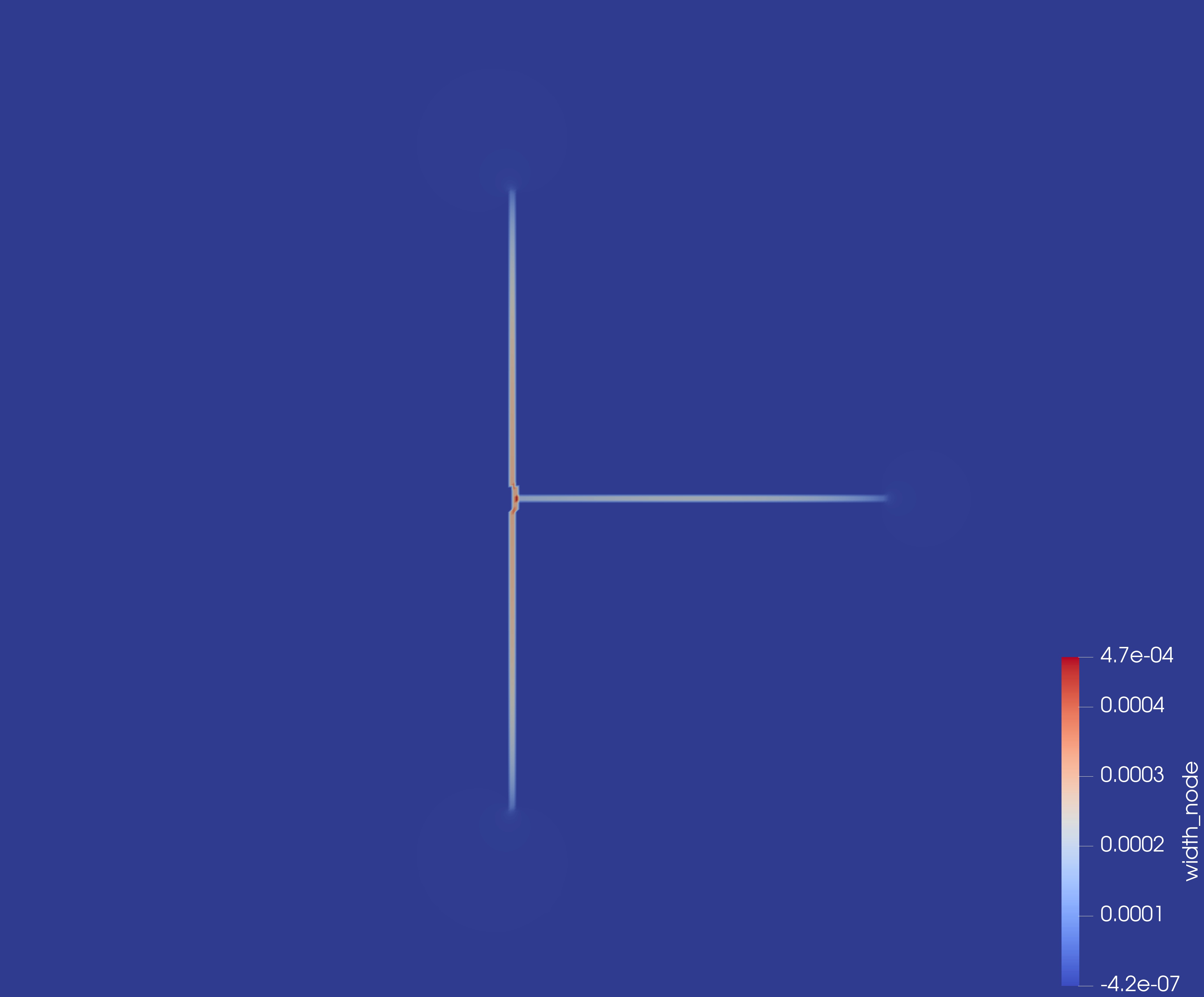


Fig. 18(a) shows the pressure responses for two interface toughness with . These two responses are identical in the early time until the hydraulic fracture starts interacting with the natural fracture. For , we see a sudden drop when the hydraulic fracture branches along the interface. Once the branched fractures reach the reservoir media, the pressure starts to increase. In contrast, for , we see only a slight pressure drop when the hydraulic fracture bypasses the weak interface but then it follows back the original pressure decline trend.
With , the natural fracture attracts the hydraulic fracture as shown in Figs. 19(a) and 20(a). The smaller , the easier and earlier the hydraulic fracture is attracted into the natural fracture (18(b)). After the hydraulic fracture propagates through the natural fracture, the pressure increases until the propagation resumes in the reservoir media (see Figs. 19(a) and 20(a)).


The distributions of Biot’s coefficient also show a sharp change in the vicinity of developed hydraulic fracture and a smooth transition in the crack tip. The examples demonstrate that our approaches for width Eq. (44) and crack normal vector Eq. (45) computations are well applicable to complex hydraulic fractures.
6 Conclusions
In this paper, we proposed a hydro-mechanical phase-field model with diffused poroelasticity derived from micromechanical analysis. Our proposed Biot’s parameters depend not only on the phase-field variable but also on the type of energy decomposition, and the poroelastic strain energy is degraded through Biot’s parameters rather than degrading the fluid pressure terms. The theoretical analysis shows that our proposed model automatically ensures the stress continuity on the crack interface (i.e., with ). Our proposed model was compared against the three commonly-used phase-field models for poroelastic media, and it can more accurately recover crack opening displacements irrespective of the pressure profile or Biot’s coefficient. The proposed model was also verified against the KGD fracture solution in the toughness-dominated regime. Furthermore, we simulated hydraulic fracture interactions with a natural fracture to demonstrate its capability for dealing with complex hydraulic fracture behaviours.
The proposed model is implemented in an open source code, OpenGeoSys [6]. As future study, the model is to be extended for thermo-hydro-mechanical and phase-field coupling problems. On the other hand, to deal with the loss of local mass conservation of fluid for the traditional continuous Galerkin finite element method, the mixed finite element method [38] or enriched Galerkin finite element method [56] may be needed in the future.
CRediT author statement
All authors have contributed equally.
Acknowledgments
The authors gratefully acknowledge the funding provided by the Deutsche Forschungsgemeinschaft (DFG, German Research Foundation), Germany through the HIGHER project (Grant No. PA 3451/1-1). TY’s contribution is funded by the China and Germany Postdoctoral Exchange Program (Grant No. ZD202137) and the National Natural Science Foundation of China (Grant No. 12202137). The first author (TY) would like to express his gratitude to Dr. Mostafa Mollaali for his help in visualization and Dr. Yijun Chen for the informative discussions.
Conflict of interest
The authors declare that they have no known competing financial interests or personal relationships that could have appeared to influence the work reported in this paper.
References
- Alessi et al., [2017] Alessi, R., Marigo, J. J., Maurini, C., and Vidoli, S. (2017). Coupling damage and plasticity for a phase-field regularisation of brittle, cohesive and ductile fracture: One-dimensional examples. International Journal of Mechanical Sciences, pages 1–18.
- Ambati et al., [2014] Ambati, M., Gerasimov, T., and De Lorenzis, L. (2014). A review on phase-field models of brittle fracture and a new fast hybrid formulation. Computational Mechanics, 55(2):383–405.
- Ambati et al., [2015] Ambati, M., Gerasimov, T., and De Lorenzis, L. (2015). Phase-field modeling of ductile fracture. Computational Mechanics, 55(5):1017–1040.
- Amor et al., [2009] Amor, H., Marigo, J.-J., and Maurini, C. (2009). Regularized formulation of the variational brittle fracture with unilateral contact: Numerical experiments. Journal of the Mechanics and Physics of Solids, 57(8):1209 – 1229.
- Balay et al., [2019] Balay, S., Abhyankar, S., Adams, M., Brown, J., Brune, P., Buschelman, K., Dalcin, L., Dener, A., Eijkhout, V., Gropp, W., et al. (2019). Petsc users manual.
- Bilke et al., [2022] Bilke, L., Fischer, T., Naumov, D., Lehmann, C., Lu, R., Meng, B., Rink, K., Grunwald, N., Buchwald, J., Silbermann, C., Habel, R., Günther, L., Mollaali, M., Meisel, T., Randow, J., Einspänner, S., Shao, H., Kurgyis, K., Kolditz, O., and Garibay, J. (2022). Opengeosys.
- Biot, [1941] Biot, M. (1941). General theory of three-dimensional consolidation. Journal of Applied Physics, 12(2):155–164.
- Biot, [1962] Biot, M. A. (1962). Mechanics of deformation and acoustic propagation in porous media. Journal of applied physics, 33(4):1482–1498.
- Borden et al., [2012] Borden, M., Verhoosel, C., Scott, M., Hughes, T., and Landis, C. (2012). A phase-field description of dynamic brittle fracture. Computer Methods in Applied Mechanics and Engineering, 217-220:77–95.
- Bourdin, [2007] Bourdin, B. (2007). Numerical implementation of the variational formulation for quasi-static brittle fracture. Interfaces and free boundaries, 9(3):411–430.
- Bourdin et al., [2012] Bourdin, B., Chukwudozie, C., and Yoshioka, K. (2012). A variational approach to the numerical simulation of hydraulic fracturing. In SPE ATCE.
- Bourdin et al., [2000] Bourdin, B., Francfort, G., and Marigo, J.-J. (2000). Numerical experiments in revisited brittle fracture. J. Mech. and Phys. of Solids, 48(4):797–826.
- Bourdin et al., [2008] Bourdin, B., Francfort, G., and Marigo, J.-J. (2008). The variational approach to fracture. Journal of Elasticity, 91(1-3):5–148.
- Bourdin et al., [2011] Bourdin, B., Larsen, C., and Richardson, C. (2011). A time-discrete model for dynamic fracture based on crack regularization. International Journal of Fracture, 168(2):133–143.
- Bourdin et al., [2014] Bourdin, B., Marigo, J. J., Maurini, C., and Sicsic, P. (2014). Morphogenesis and propagation of complex cracks induced by thermal shocks. Physical Review Letters, 112(1):1–5.
- Bryant and Sun, [2021] Bryant, E. C. and Sun, W. (2021). Phase field modeling of frictional slip with slip weakening/strengthening under non-isothermal conditions. Computer Methods in Applied Mechanics and Engineering, 375:113557.
- Budiansky and O’connell, [1976] Budiansky, B. and O’connell, R. J. (1976). Elastic moduli of a cracked solid. Int. J. Solids Struct., 12(2):81–97.
- Burke et al., [2013] Burke, S., Ortner, C., and Süli, E. (2013). An adaptive finite element approximation of a generalized ambrosio–tortorelli functional. Mathematical Models and Methods in Applied Sciences, 23(09):1663–1697.
- Cajuhi et al., [2017] Cajuhi, T., Sanavia, L., and De Lorenzis, L. (2017). Phase-field modeling of fracture in variably saturated porous media. Computational Mechanics, pages 1–20.
- Carrara et al., [2020] Carrara, P., Ambati, M., Alessi, R., and De Lorenzis, L. (2020). A framework to model the fatigue behavior of brittle materials based on a variational phase-field approach. Computer Methods in Applied Mechanics and Engineering, 361:112731.
- Castañeda and Willis, [1995] Castañeda, P. P. and Willis, J. (1995). The effect of spatial distribution on the effective behavior of composite materials and cracked media. Journal of the Mechanics and Physics of Solids, 43(12):1919–1951.
- [22] Chen, Y., Hu, S., Wei, K., Hu, R., Zhou, C., and Jing, L. (2014a). Experimental characterization and micromechanical modeling of damage-induced permeability variation in beishan granite. International Journal of Rock Mechanics and Mining Sciences, 71:64–76.
- [23] Chen, Y., Hu, S., Zhou, C., and Jing, L. (2014b). Micromechanical modeling of anisotropic damage-induced permeability variation in crystalline rocks. Rock mechanics and rock engineering, 47(5):1775–1791.
- Chukwudozie et al., [2019] Chukwudozie, C., Bourdin, B., and Yoshioka, K. (2019). A variational phase-field model for hydraulic fracturing in porous media. Computer Methods in Applied Mechanics and Engineering, 347:957–982.
- Chukwudozie, [2016] Chukwudozie, C. P. (2016). Application of the Variational Fracture Model to Hydraulic Fracturing in Poroelastic Media. PhD thesis, Louisiana State University.
- Costa et al., [2022] Costa, A., Cusini, M., Jin, T., Settgast, R., and Dolbow, J. E. (2022). A multi-resolution approach to hydraulic fracture simulation. International Journal of Fracture, 237(1-2):165–188.
- Coussy, [2004] Coussy, O. (2004). Poromechanics. John Wiley & Sons.
- Cui et al., [2021] Cui, C., Ma, R., and Martínez-Pañeda, E. (2021). A phase field formulation for dissolution-driven stress corrosion cracking. Journal of the Mechanics and Physics of Solids, 147:104254.
- Cusini et al., [2021] Cusini, M., White, J. A., Castelletto, N., and Settgast, R. R. (2021). Simulation of coupled multiphase flow and geomechanics in porous media with embedded discrete fractures. International Journal for Numerical and Analytical Methods in Geomechanics, 45(5):563–584.
- de Borst and Verhoosel, [2016] de Borst, R. and Verhoosel, C. V. (2016). Gradient damage vs phase-field approaches for fracture: Similarities and differences. Computer Methods in Applied Mechanics and Engineering, 312:78–94.
- De Lorenzis and Maurini, [2021] De Lorenzis, L. and Maurini, C. (2021). Nucleation under multi-axial loading in variational phase-field models of brittle fracture. International Journal of Fracture, pages 1–21.
- Detournay and Garagash, [2003] Detournay, E. and Garagash, D. (2003). The near-tip region of a fluid-driven fracture propagating in a permeable elastic solid. Journal of Fluid Mechanics, 494:1–32.
- Dormieux and Kondo, [2005] Dormieux, L. and Kondo, D. (2005). Poroelasticity and damage theory for saturated cracked media. In Applied micromechanics of porous materials, pages 153–186. Springer.
- Dormieux et al., [2006] Dormieux, L., Kondo, D., and Ulm, F.-J. (2006). Microporomechanics. John Wiley & Sons.
- Ehlers and Luo, [2017] Ehlers, W. and Luo, C. (2017). A phase-field approach embedded in the Theory of Porous Media for the description of dynamic hydraulic fracturing. Computer Methods in Applied Mechanics and Engineering, 315:348–368.
- Eshelby, [1957] Eshelby, J. D. (1957). The determination of the elastic field of an ellipsoidal inclusion, and related problems. Proceedings of the royal society of London. Series A. Mathematical and physical sciences, 241(1226):376–396.
- Fei and Choo, [2020] Fei, F. and Choo, J. (2020). A phase-field method for modeling cracks with frictional contact. International Journal for Numerical Methods in Engineering, 121(4):740–762.
- Feng et al., [2021] Feng, Y., Haugen, K., and Firoozabadi, A. (2021). Phase-field simulation of hydraulic fracturing by co2, water and nitrogen in 2d and comparison with laboratory data. Journal of Geophysical Research: Solid Earth, 126(11):e2021JB022509.
- Francfort and Marigo, [1998] Francfort, G. and Marigo, J.-J. (1998). Revisiting brittle fracture as an energy minimization problem. J. Mech. and Phys. of Solids, 46(8):1319–1342.
- Freddi, [2019] Freddi, F. (2019). Fracture energy in phase field models. Mechanics Research Communications, 96:29–36.
- Freddi and Royer-Carfagni, [2010] Freddi, F. and Royer-Carfagni, G. (2010). Regularized variational theories of fracture: A unified approach. Journal of the Mechanics and Physics of Solids, 58(8):1154–1174.
- Garagash, [2006] Garagash, D. I. (2006). Plane-strain propagation of a fluid-driven fracture during injection and shut-in: Asymptotics of large toughness. Engineering fracture mechanics, 73(4):456–481.
- Gerasimov and Lorenzis, [2019] Gerasimov, T. and Lorenzis, L. D. (2019). On penalization in variational phase-field models of brittle fracture. Computer Methods in Applied Mechanics and Engineering, 354:990–1026.
- Guo and Fall, [2019] Guo, G. and Fall, M. (2019). Modelling of preferential gas flow in heterogeneous and saturated bentonite based on phase field method. Computers and Geotechnics, 116:103206.
- Hansen-Dörr et al., [2019] Hansen-Dörr, A. C., de Borst, R., Hennig, P., and Kästner, M. (2019). Phase-field modelling of interface failure in brittle materials. Computer Methods in Applied Mechanics and Engineering, 346:25–42.
- Heider and Markert, [2017] Heider, Y. and Markert, B. (2017). A phase-field modeling approach of hydraulic fracture in saturated porous media. Mechanics Research Communications, 80:38–46.
- [47] Heider, Y. and Sun, W. (2020a). A phase field framework for capillary-induced fracture in unsaturated porous media: Drying-induced vs. hydraulic cracking. Computer Methods in Applied Mechanics and Engineering, 359:112647.
- [48] Heider, Y. and Sun, W. (2020b). A phase field framework for capillary-induced fracture in unsaturated porous media: Drying-induced vs. hydraulic cracking. Computer Methods in Applied Mechanics and Engineering, 359:112647.
- Heister et al., [2015] Heister, T., Wheeler, M., and Wick, T. (2015). A primal-dual active set method and predictor-corrector mesh adaptivity for computing fracture propagation using a phase-field approach. Computer Methods in Applied Mechanics and Engineering, 290:466–495.
- Hu and Garagash, [2010] Hu, J. and Garagash, D. (2010). Plane-strain propagation of a fluid-driven crack in a permeable rock with fracture toughness. Journal of Engineering Mechanics, 136(9):1152–1166.
- Jiang et al., [2010] Jiang, T., Shao, J., Xu, W., and Zhou, C. (2010). Experimental investigation and micromechanical analysis of damage and permeability variation in brittle rocks. International Journal of Rock Mechanics and Mining Sciences, 47(5):703–713.
- Khalil et al., [2022] Khalil, Z., Elghazouli, A. Y., and Martínez-Pañeda, E. (2022). A generalised phase field model for fatigue crack growth in elastic–plastic solids with an efficient monolithic solver. Computer Methods in Applied Mechanics and Engineering, 388:114286.
- Kienle and Keip, [2021] Kienle, D. and Keip, M.-A. (2021). A variational minimization formulation for hydraulically induced fracturing in elastic-plastic solids. International Journal of Fracture, pages 1–25.
- Kim et al., [2011] Kim, J., Tchelepi, H. A., and Juanes, R. (2011). Stability and convergence of sequential methods for coupled flow and geomechanics: Fixed-stress and fixed-strain splits. Computer Methods in Applied Mechanics and Engineering, 200(13-16):1591–1606.
- Kuhn et al., [2016] Kuhn, C., Noll, T., and Müller, R. (2016). On phase field modeling of ductile fracture. GAMM Mitteilungen, 39(1):35–54.
- Lee et al., [2016] Lee, S., Lee, Y.-J., and Wheeler, M. F. (2016). A locally conservative enriched galerkin approximation and efficient solver for elliptic and parabolic problems. SIAM Journal on Scientific Computing, 38(3):A1404–A1429.
- Lee et al., [2017] Lee, S., Wheeler, M., and Wick, T. (2017). Iterative coupling of flow, geomechanics and adaptive phase-field fracture including level-set crack width approaches. Journal of Computational and Applied Mathematics, 314:40–60.
- Li and Zhou, [2019] Li, K. and Zhou, S. (2019). Numerical investigation of multizone hydraulic fracture propagation in porous media: New insights from a phase field method. Journal of Natural Gas Science and Engineering, 66:42–59.
- Li et al., [2021] Li, P., Li, D., Wang, Q., and Zhou, K. (2021). Phase-field modeling of hydro-thermally induced fracture in thermo-poroelastic media. Engineering Fracture Mechanics, 254:107887.
- Li et al., [2016] Li, T., Marigo, J.-J., Guilbaud, D., and Potapov, S. (2016). Gradient damage modeling of brittle fracture in an explicit dynamic context. International Journal for Numerical Methods in Engineering, 00(March):1–25.
- Liu et al., [2020] Liu, J., Liang, X., Xue, Y., Fu, Y., Yao, K., and Dou, F. (2020). Investigation on crack initiation and propagation in hydraulic fracturing of bedded shale by hybrid phase-field modeling. Theoretical and Applied Fracture Mechanics, 108:102651.
- Lorentz and Godard, [2011] Lorentz, E. and Godard, V. (2011). Gradient damage models: Toward full-scale computations. Computer Methods in Applied Mechanics and Engineering, 200(21-22):1927–1944.
- Luo et al., [2023] Luo, C., Sanavia, L., and De Lorenzis, L. (2023). Phase-field modeling of drying-induced cracks: Choice of coupling and study of homogeneous and localized damage. Computer Methods in Applied Mechanics and Engineering, 410:115962.
- Martínez-Pañeda et al., [2018] Martínez-Pañeda, E., Golahmar, A., and Niordson, C. F. (2018). A phase field formulation for hydrogen assisted cracking. Computer Methods in Applied Mechanics and Engineering, 342:742–761.
- Maurini et al., [2013] Maurini, C., Bourdin, B., Gauthier, G., and Lazarus, V. (2013). Crack patterns obtained by unidirectional drying of a colloidal suspension in a capillary tube: Experiments and numerical simulations using a two-dimensional variational approach. International Journal of Fracture, 184(1-2):75–91.
- Mesgarnejad et al., [2015] Mesgarnejad, A., Bourdin, B., and Khonsari, M. (2015). Validation simulations for the variational approach to fracture. Computer Methods in Applied Mechanics and Engineering, 290:420–437.
- Miehe et al., [2010] Miehe, C., Hofacker, M., and Welschinger, F. (2010). A phase field model for rate-independent crack propagation: Robust algorithmic implementation based on operator splits. Computer Methods in Applied Mechanics and Engineering, 199(45):2765–2778.
- Miehe and Mauthe, [2016] Miehe, C. and Mauthe, S. (2016). Phase field modeling of fracture in multi-physics problems. part iii. crack driving forces in hydro-poro-elasticity and hydraulic fracturing of fluid-saturated porous media. Computer Methods in Applied Mechanics and Engineering, 304:619–655.
- Miehe et al., [2015] Miehe, C., Mauthe, S., and Teichtmeister, S. (2015). Minimization principles for the coupled problem of darcy–biot-type fluid transport in porous media linked to phase field modeling of fracture. Journal of the Mechanics and Physics of Solids, 82:186–217.
- [70] Mikelić, A., Wheeler, M., and Wick, T. (2015a). A Phase-Field method for propagating fluid-filled fractures coupled to a surrounding porous medium. Multiscale Modeling & Simulation, 48(1):162–186.
- [71] Mikelić, A., Wheeler, M., and Wick, T. (2015b). A quasi-static phase-field approach to pressurized fractures. Nonlinearity, 28(5):1371–1399.
- [72] Mikelić, A., Wheeler, M., and Wick, T. (2015c). Phase-field modeling of a fluid-driven fracture in a poroelastic medium. Computational Geosciences, 19(6):1171–1195.
- Mori and Tanaka, [1973] Mori, T. and Tanaka, K. (1973). Average stress in matrix and average elastic energy of materials with misfitting inclusions. Acta metallurgica, 21(5):571–574.
- Mumford and Shah, [1989] Mumford, D. and Shah, J. (1989). Optimal approximations by piecewise smooth functions and associated variational problems. Communications on Pure and Applied Mathematics, 42(5):577–685.
- Nguyen et al., [2020] Nguyen, T.-T., Yvonnet, J., Waldmann, D., and He, Q.-C. (2020). Implementation of a new strain split to model unilateral contact within the phase field method. International Journal for Numerical Methods in Engineering, 121(21):4717–4733.
- Nguyen and Wu, [2018] Nguyen, V. P. and Wu, J.-Y. (2018). Modeling dynamic fracture of solids with a phase-field regularized cohesive zone model. Computer Methods in Applied Mechanics and Engineering, 340:1000–1022.
- Pham et al., [2011] Pham, K., Amor, H., Marigo, J.-J., and Maurini, C. (2011). Gradient damage models and their use to approximate brittle fracture. Int. J. Damage Mech., 20(4, SI):618–652.
- Quinteros et al., [2023] Quinteros, L., García-Macías, E., and Martínez-Pañeda, E. (2023). Electromechanical phase-field fracture modelling of piezoresistive cnt-based composites. Computer Methods in Applied Mechanics and Engineering, 407:115941.
- Santillán et al., [2017] Santillán, D., Juanes, R., and Cueto-Felgueroso, L. (2017). Phase field model of fluid-driven fracture in elastic media: Immersed-fracture formulation and validation with analytical solutions. Journal of Geophysical Research: Solid Earth, 122(4):2565–2589.
- Santillán et al., [2018] Santillán, D., Juanes, R., and Cueto-Felgueroso, L. (2018). Phase field model of hydraulic fracturing in poroelastic media: Fracture propagation, arrest, and branching under fluid injection and extraction. Journal of Geophysical Research: Solid Earth, 123(3):2127–2155.
- Sargado et al., [2018] Sargado, J., Keilegavlen, E., Berre, I., and Nordbotten, J. (2018). High-accuracy phase-field models for brittle fracture based on a new family of degradation functions. Journal of the Mechanics and Physics of Solids, 111:458 – 489.
- Schuler et al., [2020] Schuler, L., Ilgen, A. G., and Newell, P. (2020). Chemo-mechanical phase-field modeling of dissolution-assisted fracture. Computer Methods in Applied Mechanics and Engineering, 362:112838.
- Seiler et al., [2018] Seiler, M., Hantschke, P., Brosius, A., and Kästner, M. (2018). A numerically efficient phase-field model for fatigue fracture - 1D analysis. Pamm, 18(1):e201800207.
- Sneddon and Lowengrub, [1969] Sneddon, I. and Lowengrub, M. (1969). Crack problems in the classical theory of elasticity. The SIAM series in Applied Mathematics. John Wiley & Sons.
- Tanné et al., [2018] Tanné, E., Li, T., Bourdin, B., Marigo, J.-J., and Maurini, C. (2018). Crack nucleation in variational phase-field models of brittle fracture. J. Mech. Phys. Solids, 110:80–99.
- Ulloa et al., [2022] Ulloa, J., Noii, N., Alessi, R., Aldakheel, F., Degrande, G., and François, S. (2022). Variational modeling of hydromechanical fracture in saturated porous media: A micromechanics-based phase-field approach. Computer Methods in Applied Mechanics and Engineering, 396:115084.
- van Dijk et al., [2020] van Dijk, N., Espadas-Escalante, J., and Isaksson, P. (2020). Strain energy density decompositions in phase-field fracture theories for orthotropy and anisotropy. International Journal of Solids and Structures, 196-197:140–153.
- Wang, [2000] Wang, H. F. (2000). Theory of linear poroelasticity with applications to geomechanics and hydrogeology, volume 2. Princeton university press.
- Wheeler et al., [2014] Wheeler, M., Wick, T., and Wollner, W. (2014). An augmented-Lagrangian method for the phase-field approach for pressurized fractures. Computer Methods in Applied Mechanics and Engineering, 271:69–85.
- Wheeler et al., [2020] Wheeler, M. F., Wick, T., and Lee, S. (2020). Ipacs: Integrated phase-field advanced crack propagation simulator. an adaptive, parallel, physics-based-discretization phase-field framework for fracture propagation in porous media. Computer Methods in Applied Mechanics and Engineering, 367:113124.
- Wilson and Landis, [2016] Wilson, Z. and Landis, C. (2016). Phase-field modeling of hydraulic fracture. Journal of the Mechanics and Physics of Solids, 96:264–290.
- Wu, [2017] Wu, J.-Y. (2017). A unified phase-field theory for the mechanics of damage and quasi-brittle failure. Journal of the Mechanics and Physics of Solids, 103:72 – 99.
- Wu and Chen, [2021] Wu, J.-Y. and Chen, W.-X. (2021). Phase-field modeling of electromechanical fracture in piezoelectric solids: Analytical results and numerical simulations. Computer Methods in Applied Mechanics and Engineering, 387:114125.
- Wu and Hong, [2023] Wu, J.-Y. and Hong, Y.-F. (2023). Crack nucleation and propagation of electromagneto-thermo-mechanical fracture in bulk superconductors during magnetization. Journal of the Mechanics and Physics of Solids, 172:105168.
- Wu and Nguyen, [2018] Wu, J.-Y. and Nguyen, V. P. (2018). A length scale insensitive phase-field damage model for brittle fracture. Journal of the Mechanics and Physics of Solids, 119:20–42.
- Xie et al., [2012] Xie, N., Zhu, Q.-Z., Shao, J.-F., and Xu, L.-H. (2012). Micromechanical analysis of damage in saturated quasi brittle materials. International Journal of Solids and Structures, 49(6):919–928.
- Xu et al., [2022] Xu, W., Yu, H., Zhang, J., Lyu, C., Wang, Q., Micheal, M., and Wu, H. (2022). Phase-field method of crack branching during sc-co2 fracturing: A new energy release rate criterion coupling pore pressure gradient. Computer Methods in Applied Mechanics and Engineering, 399:115366.
- Xu et al., [2023] Xu, Y., You, T., and Zhu, Q. (2023). Reconstruct lower-dimensional crack paths from phase-field point cloud. International Journal for Numerical Methods in Engineering, pages 1–24.
- Yang et al., [2018] Yang, Y., Tang, X., Zheng, H., Liu, Q., and Liu, Z. (2018). Hydraulic fracturing modeling using the enriched numerical manifold method. Applied Mathematical Modelling, 53:462–486.
- Yi et al., [2020] Yi, L.-P., Waisman, H., Yang, Z.-Z., and Li, X.-G. (2020). A consistent phase field model for hydraulic fracture propagation in poroelastic media. Computer Methods in Applied Mechanics and Engineering, 372:113396.
- Yin and Kaliske, [2020] Yin, B. and Kaliske, M. (2020). A ductile phase-field model based on degrading the fracture toughness: Theory and implementation at small strain. Computer Methods in Applied Mechanics and Engineering, 366:113068.
- Yoshioka and Bourdin, [2016] Yoshioka, K. and Bourdin, B. (2016). A variational hydraulic fracturing model coupled to a reservoir simulator. International Journal of Rock Mechanics and Mining Sciences, 88:137–150.
- Yoshioka et al., [2021] Yoshioka, K., Mollaali, M., and Kolditz, O. (2021). Variational phase-field fracture modeling with interfaces. Computer Methods in Applied Mechanics and Engineering, 384:113951.
- Yoshioka et al., [2020] Yoshioka, K., Naumov, D., and Kolditz, O. (2020). On crack opening computation in variational phase-field models for fracture. Computer Methods in Applied Mechanics and Engineering, 369:113210.
- Zaoui, [2002] Zaoui, A. (2002). Continuum micromechanics: survey. J. Eng. Mech., 128(8):808–816.
- Zhang et al., [2023] Zhang, D., Yi, L., Yang, Z., Li, X., and Zhang, F. (2023). Phase field model for simulating hydraulic fracture propagation and oil–water two-phase flow in reservoir. Computer Methods in Applied Mechanics and Engineering, 404:115838.
- Zhou et al., [2018] Zhou, S., Zhuang, X., and Rabczuk, T. (2018). A phase-field modeling approach of fracture propagation in poroelastic media. Engineering Geology, 240:189–203.
- Zhou et al., [2019] Zhou, S., Zhuang, X., and Rabczuk, T. (2019). Phase-field modeling of fluid-driven dynamic cracking in porous media. Computer Methods in Applied Mechanics and Engineering, 350:169–198.
- Zhu et al., [2008] Zhu, Q., Kondo, D., and Shao, J. (2008). Micromechanical analysis of coupling between anisotropic damage and friction in quasi brittle materials: role of the homogenization scheme. Int. J. Solids Struct., 45(5):1385–1405.
- Zhuang et al., [2022] Zhuang, X., Li, X., and Zhou, S. (2022). Three-dimensional phase field feature of longitudinal hydraulic fracture propagation in naturally layered rocks under stress boundaries. Engineering with Computers, pages 1–24.
- Zhuang et al., [2020] Zhuang, X., Zhou, S., Sheng, M., and Li, G. (2020). On the hydraulic fracturing in naturally-layered porous media using the phase field method. Engineering Geology, 266:105306.
- Ziaei-Rad et al., [2023] Ziaei-Rad, V., Mollaali, M., Nagel, T., Kolditz, O., and Yoshioka, K. (2023). Orthogonal decomposition of anisotropic constitutive models for the phase field approach to fracture. Journal of the Mechanics and Physics of Solids, 171:105143.
- Ziaei-Rad et al., [2016] Ziaei-Rad, V., Shen, L., Jiang, J., and Shen, Y. (2016). Identifying the crack path for the phase field approach to fracture with non-maximum suppression. Computer Methods in Applied Mechanics and Engineering, 312:304–321.