Incentive Mechanism Design for Unbiased
Federated Learning with Randomized
Client Participation The work of Bing Luo was supported by the AIRS-CUHKSZ-Yale Joint Postdoctoral Fellowship. The work of Jianwei Huang was supported by National Natural Science Foundation of China (Project 62271434), Shenzhen Science and Technology Program (Project JCYJ20210324120011032), Guangdong Basic and Applied Basic Research Foundation (Project 2021B1515120008), Shenzhen Key Lab of Crowd Intelligence EmpoweredLow-Carbon Energy Network (No. ZDSYS20220606100601002), and the Shenzhen Institute of Artificial Intelligence and Robotics for Society. The work of Leandros Tassiulas was supported by ARO W911NF-23-1-0088, NSF-AoF FAIN 2132573 and NSF CNS-2112562. (Corresponding author: Jianwei Huang.)

We consider a typical FL scenario, where a central server wants to learn a model based on the data from a set $\mathcal{N}=\{1,\ldots,N\}$ clients. Each client $n\in\mathcal{N}$ has $d_{n}$ data samples, ($\boldsymbol{x}_{n,1},\ldots,\boldsymbol{x}_{n,d_{n}}$), which is distributed in a non-i.i.d. fashion. Define ${{f}\left(\boldsymbol{w};\boldsymbol{x}_{n,i}\right)}$ as the loss function, indicating how the machine learning model parameter $\boldsymbol{w}$ performs on the data sample $\boldsymbol{x}_{n,i}$. Thus, the local loss function of client $n$ is

We further denote $a_{n}={d_{n}}/{\sum\nolimits_{n=1}^{N}\!d_{n}}$ as the weight of the $n$-th device, where $\sum\nolimits_{n=1}^{N}a_{n}=1$. By denoting $F\left(\boldsymbol{w}\right)$ as the global loss function, the goal of FL is to solve the following optimization problem [1]:

Due to limited system bandwidth and clients’ diverse availability, the most popular and de facto optimization algorithm to solve (2) is FedAvg [2]. In FedAvg, the server randomly samples a fraction of $K$ clients (known as partial client participation) in each round, and each selected client performs multiple (e.g., $E$) steps of local stochastic gradient descent (SGD) iterations on (1). Then, the server aggregates their resulting local model updates periodically for a given deadline of $R$ rounds or until the global loss (2) converges.

However, considering that clients in FL are independent decision-makers, each client $n$ can decide its own participation level (probability) $q_{n}$, instead of using the sampling probability decided by the server. Nevertheless, without a careful algorithm design, the obtained global model can be severely biased due to statistical heterogeneity.

In the following, before we present our incentive mechanism design, we first propose an unbiased model aggregation scheme under an arbitrary independent client participation level $\boldsymbol{q}\!=\!\{q_{1},\ldots,q_{N}\}$, such that the obtained model based on our mechanism is unbiased towards full client participation. We define the weighted aggregated model with full client participation for any round $r$ as $\overline{\boldsymbol{w}}^{r+1}:=\sum\nolimits_{n=1}^{N}a_{n}\boldsymbol{w}_{n}^{r+1}$. With this, we have the following result.

Remark: The interpretation of our aggregation scheme is similar to that of importance sampling. More specifically, we inversely re-weight the participant’s updated model gradient in the aggregation step (e.g., $\frac{1}{q_{n}}$ for client $n$), such that the aggregated model is unbiased towards the true update with full client participation. We note that simply inversely weighting the model updates from the sampled clients does not yield an unbiased global model, i.e. $\mathbb{E}_{\mathcal{K}(\boldsymbol{q})^{(r)}}[\sum_{i\in\mathcal{K}(\boldsymbol{q})^{(r)}}\frac{p_{i}}{Kq_{i}}\mathbf{w}_{i}^{(r+1)}]\neq\overline{\mathbf{w}}^{(r+1)}$, as the equality holds only when clients are sampled uniformly at random, i.e., ${q_{i}}=1/N$. Particularly, when $q_{n}=1$ for all $n$, $\mathcal{S}(\boldsymbol{q})^{r}$ is the full set with all $N$ clients, and $\boldsymbol{w}^{r+1}$ in (3) recovers $\overline{\boldsymbol{w}}^{r+1}$. Nevertheless, unlike most active sampling schemes (e.g., [15, 16, 17, 22]) where clients’ sampling probabilities $q_{n}^{\text{sam}}$ are dependent with $\sum_{n=1}^{N}q_{n}^{\text{sam}}=1$, the clients’ participation levels ${q_{n}}$ in our model is independent from each other with the sum $\sum_{n=1}^{N}q_{n}$ varying between $0$ to $N$.

As clients are independent decision-makers, we will explore the impact of clients’ independent participation levels (probabilities) $\boldsymbol{q}=\{q_{1},\ldots,q_{N}\}$ in the incentive mechanism design. Specifically, under a limited payment budget, the server designs a customized pricing scheme for each client’s participation level to maximize the model performance. In the following, we present the decision problems for the server and the clients.

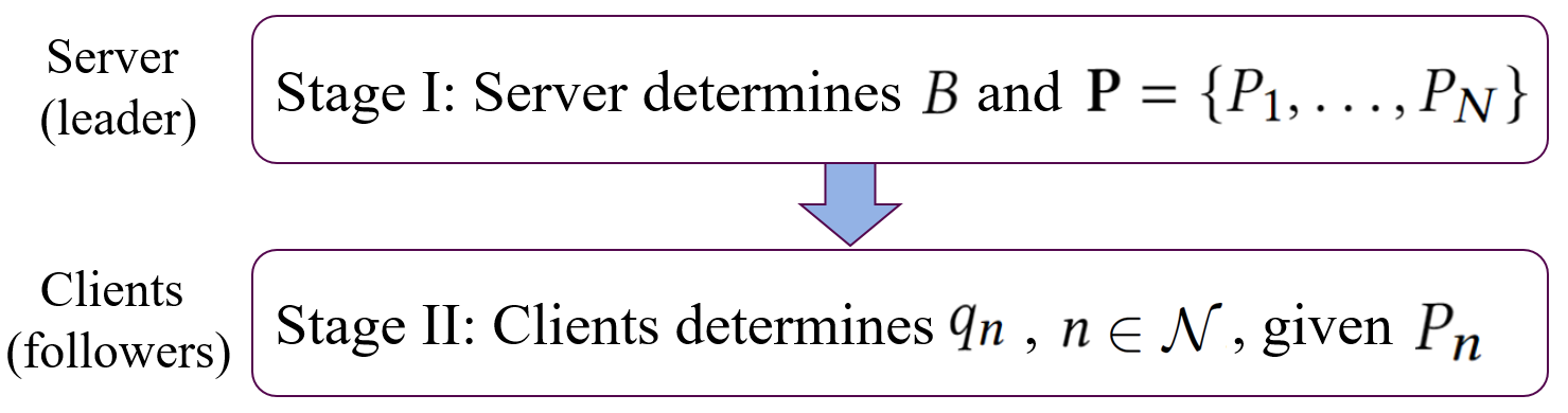
As shown in Fig. 2, we model the sequential decision-making between the server and clients as a two-stage Stackelberg game [29], where the server acts as the Stackelberg leader and decides the pricing variables $\boldsymbol{P}=\{P_{1},\ldots,P_{N}\}$ to minimize its utility defined in (5a) in Stage I. Then, given the server’s pricing strategy $\boldsymbol{P}$, each client acts as a Stackelberg follower and chooses its reactive participation level $q_{n}$ to maximize its utility defined in (8a) in Stage II. In the following, we refer to the proposed Stackelberg game as Client Participation Level Game (CPL Game).¹¹ 1 Our mechanism assumes complete information, focusing on evaluating clients’ contribution and designing an effective payment scheme. For the more realistic incomplete information scenario, we can adopt Bayesian method to model and analyze the performance similarly with a higher complexity.

Assumptions 1 and 2 are commonly made in many existing studies of convex FL problems, such as $\ell_{2}$-norm regularized linear regression, logistic regression (e.g., [16, 31, 18, 32, 17, 21]). Nevertheless, in Assumption 3, we make an assumption for each client n with the bound $G_{n}$ instead of the bound $G$ for all the clients as in [16, 31, 18, 32, 17, 21]. This is because if clients’ data are i.i,d., then $G_{n}$ would be the same across the clients since each client locally performs SGD from the same data distribution. However, when clients have non-i.i.d. data distribution, the values of $G_{n}$ would be different, which not only characterizes the data heterogeneity in our convergence result but also yields a more accurate pricing design (as we will show in Section V). In practice, we can estimate $G_{n}$ by letting the participated clients send back their actual local stochastic gradient norms computed along the trajectory of the model updates.

We first present the introduced variance of the aggregated model $\boldsymbol{w}^{r+1}$ in (3) due to randomized client participation.

Remark: When $q_{n}=1$ for all $n$, the variance in (10) is equal to zero, since the aggregated model $\boldsymbol{w}^{r+1}$ in the left hand side of (10) is the same as $\overline{\boldsymbol{w}}^{r+1}$ because $q_{n}=1$ implies full participation.

We summarize the key insights of Theorem 1 as follows:

• •

  The bound in (11) is valid for arbitrary independent client participating level $\boldsymbol{q}$ and variant number of participating clients in each round (i.e., $\sum_{n=1}^{N}q_{n}$ can vary between $0$ to $N$), which is the key difference from existing convergence results with active client sampling [22, 15, 16, 17, 19, 18, 21].

• •

  The bound in (11) characterizes how randomized partial client participation (i.e., $q_{n}<1$) worsens the convergence rate compared to full client participation. It also indicates that in order to obtain an unbiased global model, all clients need to participate with non-zero probability for model convergence, i.e., $q_{n}>0$, for all $n$. This is because when $q_{n}\rightarrow 0$, it will take infinite number of rounds $R$ for convergence. Our bound also explains why only incentivizing and training part of the clients in existing mechanisms (e.g., [7, 8, 9, 10, 11, 12, 13, 14]) may fail to converge to the optimal global model.

• •

  The convergence bound in (11) establishes the relationship between the expected loss function $\mathbb{E}[F\left(\boldsymbol{w}^{R}(\boldsymbol{q})\right)]$, clients’ participation level $\boldsymbol{q}$, and their heterogeneous data $a_{n}G_{n}$. In other words, how clients’ unbalanced data ($a_{n}$) and non-i.i.d. data distribution ($G_{n}$) affect the model training. This not only provides analytical utility expressions for the server $U_{s}$ and clients $U_{n}$, but also enables an efficient pricing strategy as we will show in Section V.

The use of $G_{i}$ in our convergence analysis (instead of more accurate instantaneous gradient norms) is mainly due to the challenging “chicken and egg” problem. Specifically, before the model has been fully trained, it is generally impossible to know exactly how different FL configurations (e.g., clients’ different participation levels in this paper) affect the FL performance. Therefore, to optimize the FL performance, we need to have a lightweight surrogate that can (approximately) predict what will happen if we choose a specific configuration. A common surrogate used for this purpose is the convergence upper bound, which has become a common practice in the communications and networking community (e.g., [33, 22, 34, 35, 36, 37]). Moreover, our experiments in Section VI demonstrate the superiority of our designed pricing scheme based on the convergence bound, in terms of achieving higher global model performance and higher client profits compared to baseline schemes.

We approximate $\mathbb{E}[F\left(\boldsymbol{w}^{R}(\boldsymbol{q})\right)]$ with the convergence bound in (11), and rewrite client $n$’s problem given the server’s pricing strategy $\boldsymbol{P}$ as the following Problem P2^′:

We observe that the objective function (12a) is concave in $q_{n}$. Along with the linear constraints in (12b), we conclude that Problem P2^′ is concave. Therefore, the optimal solution of Problem P2^′ is unique, which is the best choice of $q_{n}$ to maximize its own utility.

Based on the first order condition, the optimal choice of $q_{n}^{*}(P_{n})$ for client $n$ satisfies

Although the closed form solution of $q_{n}^{*}(P_{n})$ is complicated because (13) is a cubic equation, we can show that $q_{n}^{*}(P_{n})$ is a monotonically increasing convex function in $P_{n}$.

Based on the client’s optimal solution in (13), we move to Stage I of the CPL game.

In Stage I, the server chooses its pricing strategy based on all the clients’ best responses. In other words, the server substitutes $q_{n}^{*}(P_{n})$ into its utility function in (5) for obtaining the optimal price vector $\boldsymbol{P}$ under the budget constraint $B$.

However, since the analytical expression of $q_{n}(P_{n})$ is complicated, it is difficult to obtain the optimal $\boldsymbol{P}$ in the server’s decision problem. As $q_{n}^{\ast}(P_{n})$ is unique, we can write its inverse function based on (13), i.e., $P_{n}(q_{n})=2c_{n}q_{n}-{a_{n}^{2}G_{n}^{2}}/{q_{n}^{2}}$. Then, we substitute this expression of $P_{n}(q_{n})$ into the server’s utility function and solve Stage I problem in (5). Therefore, with the obtained convergence bound and the constraints of $q_{n}$, we rewrite problem in (5) as the following Problem P1^′:

Although the objective function in (14a) is convex in $q_{n}$, the budget constraint in (14b) is not convex in $q_{n}$. Thus, Problem P1^′ is non-convex. To efficiently solve Problem P1^′, we define a new control variable

where $0\leq M\leq\sum_{n=1}^{N}c_{n}$. Then, we rewrite Problem P1^′ as the following Problem P1^′′:²² 2 We omit constants $F^{*}$ and $\beta$ in the objective of P1^′ for simplicity.

For any fixed feasible value of $M$, Problem P1^′′ is convex because the objective function and the constraints are convex. Hence, we can approximately solve Problem P1^′′ in two steps. First, for any fixed $M$, we solve for the optimal $\boldsymbol{q}^{*}(M)$ in Problem P1^′′ via a convex optimization tool, e.g., CVX [38]. This allows us to write the objective function of Problem P1^′′ as $g(\boldsymbol{q}^{\ast}(M),M)$. Then we will further solve the problem by using a linear search method with a fixed step-size $\epsilon_{0}$ over the interval $\left[0,\sum_{n=1}^{N}c_{n}{q_{n,\text{max}}^{2}}\right]$, which leads to $\boldsymbol{q}^{*}(M^{*}(\epsilon_{0}))=\arg\min_{M(\epsilon_{0})}\boldsymbol{q}^{*}(M(\epsilon_{0}))$.

Once we obtain $\boldsymbol{q}^{*}$ from Problem P1^′′, we immediately have the optimal price $\boldsymbol{P}^{*}$ via (13) as follows,

Finally, we conclude that the obtained solution pair $\{\boldsymbol{q}^{*},\boldsymbol{P}^{*}\}$ based on backward induction are the SE $\{\boldsymbol{P}^{{\text{SE}}},\boldsymbol{q}^{{\text{SE}}}\}$ for the proposed CPL game [29]. Notably, based on the relationship between $q_{n}^{{\text{SE}}}$ and $P_{n}^{{\text{SE}}}$ in (17), we highlight that clients with low participation level $q_{n}^{{\text{SE}}}$ will receive a low price $P_{n}^{{\text{SE}}}$, which leads to a low payment $P_{n}^{{\text{SE}}}q_{n}^{{\text{SE}}}$ from the server. In particular, if these clients with low participation levels also have high intrinsic value $v_{n}$, they may need to pay for the server, i.e., $P_{n}^{\text{SE}}<0$, which we show in the next section.

This subsection presents some interesting properties of the obtained SE $\{\boldsymbol{P}^{\text{SE}},\boldsymbol{q}^{\text{SE}}\}$. Before that, we first give the following lemma which leads to our property analysis.

We first compare the performance of our proposed optimal pricing with other benchmark pricing schemes, and then we evaluate the impact of different system parameters on the model performance and Equilibrium solution. For all three setups, we average each experiment over $20$ independent runs.

Substituting (3) into (4), we have

where $n$ in the first equation is a random variable in the randomly sampled set $\mathcal{S}(q)^{(r)}$, which concludes the proof.

Following a similar proof of convergence under full client participation [16, 32], we first show the convergence result under full client participation is $\mathbb{E}[F\left(\overline{\boldsymbol{w}}^{R})\right)]\!-\!F^{*}\leq{\beta}/{R}$, where $\mathbb{E}[F\left(\overline{\boldsymbol{w}}^{R})\right)]$ is the expected global loss after $R$ rounds with full participation, and $\beta$ is the same as in (11). Then, we use mathematical induction to obtain a non-recursive bound on $\mathbb{E}_{\mathcal{S}(\boldsymbol{q})^{r}}\left\|\boldsymbol{w}^{R}-{\boldsymbol{w}}^{*}\right\|^{2}$, and show that its difference compared to the bound of full participation $\mathbb{E}\left\|\overline{\boldsymbol{w}}^{R}-{\boldsymbol{w}}^{*}\right\|^{2}$ is the variance introduced in (10). After that, we converted the bound of $\mathbb{E}_{\mathcal{S}(\boldsymbol{q})^{r}}\left\|\boldsymbol{w}^{R}-{\boldsymbol{w}}^{*}\right\|^{2}$ to $\mathbb{E}[F\left(\boldsymbol{w}^{R}(\boldsymbol{q})\right)]-F^{*}$ using $L$-smoothness and strong convexity of $F(\cdot)$, which yields the additional term of $\alpha{\sum\nolimits_{n=1}^{N}\frac{\left(1-q_{n}\right)a_{n}^{2}G_{n}^{2}}{q_{n}}}$ in (11) compared to the upper bound with full client participation. $\hfill\square$

We write the Lagrangian function $L(\boldsymbol{q},\lambda,{\mu_{n}},{\gamma_{n}})$ of P1^′ as

where $\lambda>0$, ${\mu_{n}}\geq 0$ and $\gamma_{n}\geq 0$ are Lagrangian multipliers (dual variables). Although Problem P1^′ is non-convex, the Karush-Kuhn-Tucker (KKT) conditions are necessary for optimality. Thus, for the first order condition, we must have

Given that $0<q_{n}^{*}<q_{n,\text{max}}$, we have $\mu_{n}^{*}=0$ and $\gamma_{n}^{*}=0$ due to the Complementary Slackness in the KKT conditions, which we rewrite (21) as follows

The result is obtained since ${1}/{\lambda^{*}}$ is independent of index $n$. ∎

We exploit the relationship between $q_{n}^{*}$ and $P_{n}^{*}$ in (17), and substitute it into the first order condition (22), which leads to (18). By letting $P_{n}^{*}=0$, we have $v_{n}={1}/{(3\lambda^{*})}$. Therefore, given that $P_{n}^{*}$ in (18) decreases in $v_{n}$, we must have $P_{n}^{*}>0$ when $v_{n}<{1}/{(3\lambda^{*})}$, and $P_{n}^{*}<0$ when $v_{n}>{1}/{(3\lambda^{*})}$. Hence, we conclude the proof by letting the threshold $v^{\text{t}}={1}/{(3\lambda^{*})}$. ∎

References

- [1] P. Kairouz, H. B. McMahan, B. Avent, A. Bellet, M. Bennis, A. N. Bhagoji, K. Bonawitz, Z. Charles, G. Cormode, R. Cummings et al., “Advances and open problems in federated learning,” arXiv preprint, arXiv:1912.04977, 2019.
- [2] B. McMahan, E. Moore, D. Ramage, S. Hampson, and B. A. y Arcas, “Communication-efficient learning of deep networks from decentralized data,” in Proceedings of the 20th International Conference on Artificial Intelligence and Statistics, 2017, pp. 1273–1282.
- [3] Y. Zhan, J. Zhang, Z. Hong, L. Wu, P. Li, and S. Guo, “A survey of incentive mechanism design for federated learning,” IEEE Transactions on Emerging Topics in Computing, doi: 10.1109/TETC.2021.3063517.
- [4] R. Zeng, C. Zeng, X. Wang, B. Li, and X. Chu, “A comprehensive survey of incentive mechanism for federated learning,” arXiv preprint, arXiv:2106.15406, 2021.
- [5] M. Zhang, E. Wei, and R. Berry, “Faithful edge federated learning: Scalability and privacy,” IEEE Journal on Selected Areas in Communications, vol. 39, no. 12, pp. 3790–3804, 2021.
- [6] T. Li, A. K. Sahu, M. Zaheer, M. Sanjabi, A. Talwalkar, and V. Smith, “Federated optimization in heterogeneous networks,” in Proceedings of Machine Learning and Systems (MLSys), 2020.
- [7] W. Y. B. Lim, Z. Xiong, C. Miao, D. Niyato, Q. Yang, C. Leung, and H. V. Poor, “Hierarchical incentive mechanism design for federated machine learning in mobile networks,” IEEE Internet of Things Journal, vol. 7, no. 10, pp. 9575–9588, 2020.
- [8] J. Kang, Z. Xiong, D. Niyato, S. Xie, and J. Zhang, “Incentive mechanism for reliable federated learning: A joint optimization approach to combining reputation and contract theory,” IEEE Internet of Things Journal, vol. 6, no. 6, pp. 10 700–10 714, 2019.
- [9] N. Ding, Z. Fang, and J. Huang, “Optimal contract design for efficient federated learning with multi-dimensional private information,” IEEE Journal on Selected Areas in Communications, vol. 39, no. 1, pp. 186–200, 2020.
- [10] J. S. Ng, W. Y. B. Lim, H.-N. Dai, Z. Xiong, J. Huang, D. Niyato, X.-S. Hua, C. Leung, and C. Miao, “Joint auction-coalition formation framework for communication-efficient federated learning in uav-enabled internet of vehicles,” IEEE Transactions on Intelligent Transportation Systems, vol. 22, no. 4, pp. 2326–2344, 2020.
- [11] T. H. T. Le, N. H. Tran, Y. K. Tun, M. N. Nguyen, S. R. Pandey, Z. Han, and C. S. Hong, “An incentive mechanism for federated learning in wireless cellular networks: An auction approach,” IEEE Transactions on Wireless Communications, vol. 20, no. 8, pp. 4874–4887, 2021.
- [12] Y. Jiao, P. Wang, D. Niyato, B. Lin, and D. I. Kim, “Toward an automated auction framework for wireless federated learning services market,” IEEE Transactions on Mobile Computing, vol. 20, no. 10, pp. 3034–3048, 2020.
- [13] R. Zeng, S. Zhang, J. Wang, and X. Chu, “Fmore: An incentive scheme of multi-dimensional auction for federated learning in mec,” in Proceedings of the IEEE International Conference on Distributed Computing Systems (ICDCS), 2020, pp. 278–288.
- [14] Y. Deng, F. Lyu, J. Ren, Y.-C. Chen, P. Yang, Y. Zhou, and Y. Zhang, “Fair: Quality-aware federated learning with precise user incentive and model aggregation,” in Proceedings of the IEEE Conference on Computer Communications (INFOCOM), 2021, pp. 1–10.
- [15] H. Yang, M. Fang, and J. Liu, “Achieving linear speedup with partial worker participation in non-iid federated learning,” arXiv preprint, arXiv:2101.11203, 2021.
- [16] X. Li, K. Huang, W. Yang, S. Wang, and Z. Zhang, “On the convergence of fedavg on non-iid data,” in Proceedings of the International Conference on Learning Representation (ICLR), 2019.
- [17] Z. Qu, K. Lin, J. Kalagnanam, Z. Li, J. Zhou, and Z. Zhou, “Federated learning’s blessing: Fedavg has linear speedup,” arXiv preprint, arXiv:2007.05690, 2020.
- [18] W. Chen, S. Horvath, and P. Richtarik, “Optimal client sampling for federated learning,” arXiv preprint, arXiv:2010.13723, 2020.
- [19] E. Rizk, S. Vlaski, and A. H. Sayed, “Federated learning under importance sampling,” arXiv preprint, arXiv:2012.07383, 2020.
- [20] B. Luo, X. Li, S. Wang, J. Huang, and L. Tassiulas, “Cost-effective federated learning in mobile edge networks,” IEEE Journal on Selected Areas in Communications, vol. 39, no. 12, pp. 3606–3621, 2021.
- [21] Y. J. Cho, J. Wang, and G. Joshi, “Client selection in federated learning: Convergence analysis and power-of-choice selection strategies,” arXiv preprint, arXiv:2010.01243, 2020.
- [22] B. Luo, W. Xiao, S. Wang, J. Huang, and L. Tassiulas, “Tackling system and statistical heterogeneity for federated learning with adaptive client sampling,” in Proceedings of the IEEE Conference on Computer Communications (INFOCOM), 2022, pp. 1739–1748.
- [23] X. Tu, K. Zhu, N. C. Luong, D. Niyato, Y. Zhang, and J. Li, “Incentive mechanisms for federated learning: From economic and game theoretic perspective,” arXiv preprint, arXiv:2111.11850, 2021.
- [24] Y. Sarikaya and O. Ercetin, “Motivating workers in federated learning: A stackelberg game perspective,” IEEE Networking Letters, vol. 2, no. 1, pp. 23–27, 2019.
- [25] L. U. Khan, S. R. Pandey, N. H. Tran, W. Saad, Z. Han, M. N. Nguyen, and C. S. Hong, “Federated learning for edge networks: Resource optimization and incentive mechanism,” IEEE Communications Magazine, vol. 58, no. 10, pp. 88–93, 2020.
- [26] M. Tang and V. W. Wong, “An incentive mechanism for cross-silo federated learning: A public goods perspective,” in Proceedings of the IEEE Conference on Computer Communications (INFOCOM), 2021, pp. 1–10.
- [27] Y. Zhan and J. Zhang, “An incentive mechanism design for efficient edge learning by deep reinforcement learning approach,” in Proceedings of the IEEE Conference on Computer Communications (INFOCOM), 2020, pp. 2489–2498.
- [28] O. Candogan, K. Bimpikis, and A. Ozdaglar, “Optimal pricing in networks with externalities,” Operations Research, vol. 60, no. 4, pp. 883–905, 2012.
- [29] T. Başar and G. J. Olsder, Dynamic noncooperative game theory. SIAM, 1998.
- [30] A. Mas-Colell, M. Whinston, and J. Green, Microeconomic Theory. Oxford University Press, 1995. [Online]. Available: https://EconPapers.repec.org/RePEc:oxp:obooks:9780195102680
- [31] H. Yu, S. Yang, and S. Zhu, “Parallel restarted SGD for non-convex optimization with faster convergence and less communication,” in Proceedings of the AAAI Conference on Artificial Intelligence, 2019.
- [32] S. U. Stich, “Local SGD converges fast and communicates little,” in Proceedings of the International Conference on Learning Representation (ICLR), 2018.
- [33] S. Wang, T. Tuor, T. Salonidis, K. K. Leung, C. Makaya, T. He, and K. Chan, “Adaptive federated learning in resource constrained edge computing systems,” IEEE Journal on Selected Areas in Communications, vol. 37, no. 6, pp. 1205–1221, 2019.
- [34] L. Cui, X. Su, Y. Zhou, and J. Liu, “Optimal rate adaption in federated learning with compressed communications,” in Proceedings of the IEEE Conference on Computer Communications (INFOCOM), 2022, pp. 1459–1468.
- [35] W. Shi, S. Zhou, and Z. Niu, “Device scheduling with fast convergence for wireless federated learning,” in Proceedings of the IEEE International Conference on Communications (ICC), 2020, pp. 1–6.
- [36] J. Perazzone, S. Wang, M. Ji, and K. S. Chan, “Communication-efficient device scheduling for federated learning using stochastic optimization,” in Proceedings of the IEEE Conference on Computer Communications (INFOCOM), 2022, pp. 1449–1458.
- [37] B. Luo, X. Li, S. Wang, J. Huang, and L. Tassiulas, “Cost-effective federated learning design,” in Proceedings of the IEEE Conference on Computer Communications (INFOCOM), 2021, pp. 1–10.
- [38] S. Boyd, S. P. Boyd, and L. Vandenberghe, Convex optimization. Cambridge university press, 2004.