Remote State Estimation with Posterior-Based Stochastic Event-Triggered Schedule

Let $x$ and $y$ be two random variables with the same dimensions, the WD between them is expressed as [19]

where $\gamma(x,y)\in\{f(x,y)|\int f(x,y)dx=p(y),\int f(x,y)dy=p(x),f(x,y)\geq 0\}$. The matrix $\Gamma>0$ does not exist in the initial WD and is introduced in this paper to adjust the weight of different state components and the communication rate. When $p(x)=\phi(x;\bar{x},P_{x})$ and $p(y)=\phi(y;\bar{y},P_{y})$, it can be shown that $\mathcal{W}_{\Gamma}(x,y)$ has analytic form [20]

where $S=\Gamma^{1/2}$.

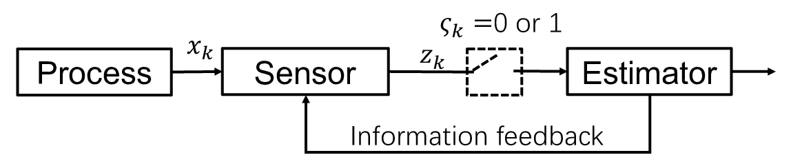
Consider the general closed-loop event-triggered estimation system shown in Fig. 1 whose dynamic model is described by

where $x_{k}\in{\mathbb{R}}^{n}$ is the system state, $z_{k}\in\mathbb{R}^{m}$ is the measurement. $w_{k}$ and $v_{k}$ are uncorrected Gaussian white noises with covariance $Q>0$ and $R>0$, respectively. The initial state $x_{0}$ is Gaussian with mean $x_{0|0}$ and covariance $P_{0|0}>0$, and is uncorrelated with $w_{k}$ and $v_{k}$. $(C,A)$ is detectable. $\varsigma_{k}=1$ denotes the sensor transmits $z_{k}$ to the estimator and $\varsigma_{k}=0$ otherwise. In this case, at moment $k$, the available information set for the estimator is

where $\mathcal{I}_{k}\triangleq\{\varsigma_{k},\varsigma_{k}z_{k}\}$ and $\mathcal{I}_{1:0}\triangleq\emptyset$. It is assumed that the feedback channel can reliably transmit data to the sensor [8].

To facilitate later analysis, let us define

where $x_{k|k-1}$ and $P_{k|k-1}$ are respectively mean and covariance of state prior PDF $p(x_{k}|\mathcal{I}_{1:k-1})$. $x_{k|k}$ and $P_{k|k}$ are respectively mean and covariance of state posterior PDF $p(x_{k}|\mathcal{I}_{1:k})$. $\tilde{x}_{k|k-1}$ and $\tilde{x}_{k|k}$ are respectively prior and posterior estimate error.

Remark 1: When the sensor transmits $z_{k}$ at each moment, the mean $x_{k|k}$ and error covariance $P_{k|k}$ of the posterior estimate are given by the standard KF [21]:

In the past, the innovation $z_{k}-z_{k|k-1}$ was often used as the basis for determining whether to trigger an event or not. Different from the innovation-based approach, a novel event-triggered idea will be proposed in this subsection. Let us start with a series of enlightening analyses. On one hand, from an information-theoretic point of view, the measurement $z_{k}$ is a function of the state $x_{k}$, and thus receiving $z_{k}$ implies more available information. On the other hand, it follows from (10) that the error covariance of KF is updated (i.e., $P_{k|k}<P_{k|k-1}$) whenever a measurement is received. From the above two aspects, it can be seen that regardless of the size of $z_{k}-z_{k|k-1}$, receiving a measurement is always better than not receiving one. This is an important feature of KF, but not considered in the innovation-based mechanism.

Let $x^{1}_{k}\triangleq x_{k}|\{\varsigma_{k}=1,z_{k},\mathcal{I}_{1:k-1}\}$ and $x^{0}_{k}\triangleq x_{k}|\{\varsigma_{k}=0,\mathcal{I}_{1:k-1}\}$ stand for the posterior estimates when $z_{k}$ is transmitted and not transmitted, respectively. Then, it follows from the above analysis that, when the divergence between $x^{0}_{k}$ and $x^{1}_{k}$ is large, $z_{k}$ is more desired to be transmitted such that $x^{0}_{k}$ can be “converted” to the better $x^{1}_{k}$. Conversely, when $x^{0}_{k}$ is very similar to $x^{1}_{k}$, the posterior estimates are almost the same whether $z_{k}$ is transmitted or not, in which case there is clearly no need to transmit $z_{k}$. This fact leads to the main idea of this paper, that is, the importance of $z_{k}$ depends on the divergence between $x^{0}_{k}$ and $x^{1}_{k}$. Following this idea, we propose a novel posterior-based SET mechanism which is expressed as

where $\vartheta_{k}$ is uniformly distributed over $[0,1]$. Theoretically, $d(x^{0}_{k},x^{1}_{k})$ can be chosen to be any metric that measures the distance between random variables (e.g., $\mathcal{W}^{2}_{\Gamma}(x^{0}_{k},x^{1}_{k})$, $\mathbb{E}[\|x^{1}_{k}-x^{0}_{k}\|^{2}]$ and $\|\mathbb{E}[x^{1}_{k}]-\mathbb{E}[x^{0}_{k}]\|^{2}$). In this paper, we choose the WD as an example for the subsequent analysis.

Notice that, $\mathcal{W}_{\Gamma}(x^{0}_{k},x^{1}_{k})$ is a complex optimization problem and so far its analytic form exists only when both $x^{0}_{k}$ and $x^{1}_{k}$ are Gaussian. Unfortunately, $x^{0}_{k}$ and $x^{1}_{k}$ represent the outputs of the estimator and are unknown. In this case, the analytic form of $\mathcal{W}_{\Gamma}(x^{0}_{k},x^{1}_{k})$ cannot be obtained and the corresponding estimator is also impossible to be derived. To avoid this, we have to give a simplified and more “analytic” metric

where $\bar{x}\triangleq\mathbb{E}[x]$, $\bar{y}\triangleq\mathbb{E}[y]$, $P_{x}\triangleq\mathbb{E}[(x-\bar{x})(x-\bar{x})^{T}]$, and $P_{y}\triangleq\mathbb{E}[(y-\bar{y})(y-\bar{y})^{T}]$. Although $\mathcal{W}_{\Gamma}(x,y)$ and $\mathcal{D}_{\Gamma}(x,y)$ seem to be different, it is fortunate that when both $x$ and $y$ are Gaussian, $\mathcal{W}_{\Gamma}(x,y)$ has the analytic form (2), which is the same as $\mathcal{D}_{\Gamma}(x,y)$. Thus, if $x^{0}_{k}$ and $x^{1}_{k}$ can be shown to be both Gaussian, then $\mathcal{D}_{\Gamma}(x^{0}_{k},x^{1}_{k})$ will be equal to the Wasserstein distance $\mathcal{W}_{\Gamma}(x^{0}_{k},x^{1}_{k})$. Inspired by this, our subsequent attention is on proving $x^{0}_{k}$ and $x^{1}_{k}$ are Gaussian in the case $d(x^{0}_{k},x^{1}_{k})$=$\mathcal{D}^{2}_{\Gamma}(x^{0}_{k},x^{1}_{k})$.

Then, the problems to be solved in later sections are summarized as follows:

• •

  Derive the analytic expressions of (11) and $p(x_{k}|\mathcal{I}_{1:k})$ under the case $d(x^{0}_{k},x^{1}_{k})=\mathcal{D}^{2}_{\Gamma}(x^{0}_{k},x^{1}_{k})$.

• •

  Analyze the performance of the proposed estimator to derive the stability conditions;

• •

  Analyze the average communication rate of the sensor to guide the selection of the adjustable parameter $\Gamma$.

In the existing works, estimators are derived with known schedulers. However, the posterior-based scheduler (11) is determined by the outputs $x^{1}_{k}$ and $x^{0}_{k}$ of the estimator, while the estimator is also determined by the posterior-based scheduler. This interconnection results in the explicit expressions for both the estimator and the scheduler are unknown, and thus the methodologies in [8, 9, 10] cannot be directly applied here. A detailed analysis of the problem is given in Theorem 1.

Theorem 1: When $d(x^{0}_{k},x^{1}_{k})=\mathcal{D}^{2}_{\Gamma}(x^{0}_{k},x^{1}_{k})$, $p(x_{k}|\mathcal{I}_{1:k})$ is Gaussian with mean $x_{k|k}$ and covariance $P_{k|k}$ which are recursively calculated by the following Kalman-like form:

Proof: Mathematical induction is used here to prove this theorem. First, the initial condition $p(x_{0}|\mathcal{I}_{1:0})=\phi(x_{0};x_{0|0},P_{0|0})$ is Gaussian. Then, it is assumed that $p(x_{k-1}|\mathcal{I}_{1:k-1})=\phi(x_{k-1};x_{k-1|k-1},P_{k-1|k-1})$ is Gaussian. Under this case, it is obvious that the prior PDF is

where the expressions for $x_{k|k-1}$ and $P_{k|k-1}$ are shown in (13) and (14).

It can be seen from (11) that $\varsigma_{k}$ is related to $x^{0}_{k}$ and $x^{1}_{k}$ only. Then, by recalling the definitions of $x^{0}_{k}$ and $x^{1}_{k}$, one knows that $\varsigma_{k}$ is essentially determined by $\mathcal{I}_{1:k-1}$ and $z_{k}$. Furthermore, since both $v_{k}$ and $w_{k}$ are white noises, the system (3) is a first-order hidden Markov model. Combining the above facts, one knows that $\varsigma_{k}$ is independent of $x_{k}$ given $(z_{k},\mathcal{I}_{1:k-1})$. In this case, it follows from Bayes rule that

Then, similar to the standard KF, one has

where

where $K_{k}$ is given in (15).

When $\varsigma_{k}=0$, utilizing Bayes rule yields

It follows from the law of total probability that

According to (11) and (20), one has

where

Notice that, $x^{0}_{k}$ is not directly related to $z_{k}$ and $\varsigma_{k}=0$ is constant. Thus, $x^{0}_{k|k}$ and $p^{0}_{k|k}$ remain invariant regardless of the value of $v_{k}$. In this case, the analytic form of (22) can be derived as

where the last equation is obtained by the fact that the integral of Gaussian PDF is equal to 1, and

Then, by substituting (18) and (24) into (21) and taking a bit of tedious but straightforward algebra, one has

where

Notice that both $\beta_{k}$ and $\bar{\beta}_{k}$ are constants with respect to $x_{k}$. Hence, according to the fact that Gaussian PDF integrals to 1, $\beta_{k}\bar{\beta}_{k}$ can be calculated by

As a result, one has

Then, let $x^{0}_{k|k}=\eta_{k}$ and place the $x^{0}_{k|k}$-related terms on the left side of the equation, one can deduce that

which means $x^{0}_{k|k}=x_{k|k-1}$. Moreover, it follows from $(P^{1}_{k|k})^{-1}=P^{-1}_{k|k-1}+C^{T}R^{-1}C$ and Lemma 1 that $U_{k}$ is simplified to

Then, utilizing the matrix inverse lemma for $U^{-1}_{k}$ yields

Both $p(x^{0}_{k})$ and $p(x^{1}_{k})$ are Gaussian, and thus $p(x_{k}|\mathcal{I}_{1:k})$ is also Gaussian. Finally, summing the above results yields (13)-(17). This completes the proof. $\square$

Theorem 1 proves that $x^{0}_{k}$ and $x^{1}_{k}$ are Gaussian, and thus $\mathcal{D}_{\Gamma}(x^{0}_{k},x^{1}_{k})$ is equivalent to $\mathcal{W}_{\Gamma}(x^{0}_{k},x^{1}_{k})$. In this case, substituting the distributions of $x^{0}_{k}$ and $x^{1}_{k}$ into (11) gives

where $\varepsilon_{k}=z_{k}-z_{k|k-1}$ and $\varrho_{k}=\mathrm{Tr}(P^{1}_{k|k}\Gamma+P^{0}_{k|k}\Gamma-2(SP^{0}_{k|k}\Gamma P^{1}_{k|k}S)^{1/2})$. As can be seen from (31), the posterior-based SET mechanism can be divided into two parts. $\|\varepsilon_{k}\|^{2}_{K^{T}_{k}\Gamma K_{k}}$ has a similar form to the innovation-based SET mechanisms, but differs in that $\|\varepsilon_{k}\|^{2}_{K^{T}_{k}\Gamma K_{k}}$ is reduced from $\|x^{1}_{k|k}-x^{0}_{k|k}\|^{2}_{\Gamma}$ and thus directly reflects the difference between the first order moments of posterior estimates. $\varrho_{k}$ represents the difference between the higher-order moments of posterior estimates, and is the most intuitive difference between the proposed SET mechanism (31) and previous SET mechanisms [8, 9, 10, 6, 11, 12, 13]. Therefore, the impact of $\varrho_{k}$ on (31) deserves to be analyzed (e.g., how much communication rate is induced by $\varrho_{k}$). The specific analysis is presented in Appendix C.

Remark 2: Deriving $\phi(x_{k};\eta_{k},U^{-1}_{k})$ inevitably makes use of information from the scheduler (11), which is determined by the unknown $x^{0}_{k}$. This means that $p(x^{0}_{k})=\phi(x_{k};\eta_{k},U^{-1}_{k})$ can actually be understood as an unsolved equation where $x^{0}_{k}$ is the unknown. In previous works [2, 3, 4, 5, 6, 7, 8, 9, 10, 11, 12, 13], the estimators were derived with the scheduler exactly known, so there is no need to solve such an equation.

For the sake of subsequent analysis, let us define

where $X>0$ and $Y>0$. Moreover, define

Theorem 2: Consider the system (3) with SET mechanism (31), if $C$ is full row rank, then $P_{k|k-1}$ in (14) is bounded by

where

where $\bar{P}_{1}\triangleq AP_{0|0}A^{T}+Q$ and $\Theta_{k}$ is defined in (32). Particularly, the matrix sequences $\{\underline{P}_{k}\}$ and $\{\bar{P}_{k}\}$ are convergent, and their limits are $P_{l}$ and $P_{u}$, respectively. Here, $P_{l}$ and $P_{u}$ are respectively the unique positive definite solutions of

where $\Theta$ is defined in (33).

Proof: First, let us derive the lower bound for $P_{k|k-1}$. It is obvious that $P_{1|0}=AP_{0|0}A^{T}+Q\geq G^{0}_{R}(AP_{0|0}A^{T}+Q)$. Assume $P_{k|k-1}\geq G^{k-1}_{R}(AP_{0|0}A^{T}+Q)$. Then, one has

where the last inequality follows from the fact $G_{Y}(X_{1})\geq G_{Y}(X_{2})$ when $X_{1}\geq X_{2}\geq 0$. Moreover, notice that $G^{1}_{R}(0)\geq G^{0}_{R}(0)$, which further yields $G^{2}_{R}(0)=G^{1}_{R}(G^{1}_{R}(0))\geq G^{1}_{R}(0)$. By analogy, we can know that $\{G^{k}_{R}(0)\}$ is a monotonic non-decreasing matrix sequence, and $G^{k}_{R}(0)\geq G^{1}_{R}(0)=Q>0$ for all $k\in{\mathbb{N}}_{++}$. Then, by mathematical induction, it can be easily deduced that $G^{k}_{R}(AP_{0|0}A^{T}+Q)\geq G^{k}_{R}(0)>0$ for all $k\in{\mathbb{N}}_{++}$. Thus far, $0<\underline{P}_{k}\leq P_{k|k-1}$ has been proved.

References

• [1] W. Liu, D. E. Quevedo, Y. Li, K. H. Johansson and B. Vucetic, “Remote State Estimation With Smart Sensors Over Markov Fading Channels,” IEEE Transactions on Automatic Control, vol. 67, no. 6, pp. 2743-2757, June 2022.
• [2] J. Wu, Q. Jia, K. H. Johansson and L. Shi, “Event-Based Sensor Data Scheduling: Trade-Off Between Communication Rate and Estimation Quality,” IEEE Transactions on Automatic Control, vol. 58, no. 4, pp. 1041-1046, April 2013.
• [3] K. You and L. Xie, “Kalman Filtering with Scheduled Measurements,” IEEE Transactions on Signal Processing, vol. 61, no. 6, pp. 1520-1530, March15, 2013.
• [4] D. Shi, T. Chen and L. Shi, “On Set-Valued Kalman Filtering and Its Application to Event-Based State Estimation,” IEEE Transactions on Automatic Control, vol. 60, no. 5, pp. 1275-1290, May 2015.
• [5] D. Shi, T. Chen, L. Shi, “An Event-Triggered Approach to State Estimation with Multiple Point and Set-Valued Measurements,” Automatica, vol. 50, pp. 1641-1648, 2014.
• [6] L. He, J. Chen and Y. Qi, “Event-Based State Estimation: Optimal Algorithm With Generalized Closed Skew Normal Distribution,” IEEE Transactions on Automatic Control, vol. 64, no. 1, pp. 321-328, Jan. 2019.
• [7] S. Trimpe and R. D’Andrea, “Event-Based State Estimation With Variance-Based Triggering,” IEEE Transactions on Automatic Control, vol. 59, no. 12, pp. 3266-3281, Dec. 2014.
• [8] D. Han, Y. Mo, J. Wu, S. Weerakkody, B. Sinopoli and L. Shi, “Stochastic Event-Triggered Sensor Schedule for Remote State Estimation,” IEEE Transactions on Automatic Control, vol. 60, no. 10, pp. 2661-2675, Oct. 2015.
• [9] M. T. Andren and A. Cervin, “Event-based state estimation using an improved stochastic send-on-delta sampling scheme,” 2016 Second International Conference on Event-based Control, Communication, and Signal Processing (EBCCSP), 2016, pp. 1-8.
• [10] E. J. Schmitt, B. Noack, W. Krippner and U. D. Hanebeck, “Gaussianity-Preserving Event-Based State Estimation With an FIR-Based Stochastic Trigger,” IEEE Control Systems Letters, vol. 3, no. 3, pp. 769-774, July 2019.
• [11] L. Li, D. Yu, Y. Xia and H. Yang, “Remote Nonlinear State Estimation With Stochastic Event-Triggered Sensor Schedule,” IEEE Transactions on Cybernetics, vol. 49, no. 3, pp. 734-745, March 2019.
• [12] S. Weerakkody, Y. Mo, B. Sinopoli, D. Han and L. Shi, “Multi-Sensor Scheduling for State Estimation With Event-Based, Stochastic Triggers,” IEEE Transactions on Automatic Control, vol. 61, no. 9, pp. 2695-2701, Sept. 2016.
• [13] A. Mohammadi and K. N. Plataniotis, “Event-Based Estimation With Information-Based Triggering and Adaptive Update,” IEEE Transactions on Signal Processing, vol. 65, no. 18, pp. 4924-4939, 15 Sept.15, 2017.
• [14] J. Wu, X. Ren, D. Han, D. Shi and L. Shi, “Finite-Horizon Gaussianity-Preserving Event-Based Sensor Scheduling in Kalman Filter Applications,” Automatica, vol. 72, pp. 100-107, Oct. 2016.
• [15] L. Xu, Y. Mo and L. Xie, “Remote State Estimation With Stochastic Event-Triggered Sensor Schedule and Packet Drops,” IEEE Transactions on Automatic Control, vol. 65, no. 11, pp. 4981-4988, Nov. 2020.
• [16] J. Huang, D. Shi and T. Chen, “Event-Triggered State Estimation With an Energy Harvesting Sensor,” IEEE Transactions on Automatic Control, vol. 62, no. 9, pp. 4768-4775, Sept. 2017.
• [17] J. Shang, H. Yu and T. Chen, “Worst-Case Stealthy Attacks on Stochastic Event-based State Estimation,” IEEE Transactions on Automatic Control, vol. 67, no. 4, pp. 2052-2059, April 2022.
• [18] M. Miskowicz M, “Send-on-delta concept: An event-based data reporting strategy,” sensors, vol. 6, no. 1, pp 49-63, 2006.
• [19] C. R. Givens and R. M. Shortt, “A Class of Wasserstein Metrics for Probability Distributions,” Michigan Mathematical Journal, vol. 32, no. 2, pp. 231-240, 1984.
• [20] O. Ingram, and F. Pukelsheim. “The Distance between Two Random Vectors with Given Dispersion Matrices,” Linear Algebra and its Applications, vol. 48, pp. 257-263, 1982.
• [21] B. Anderson and J. Moore, Optimal Filtering. Englewood Cliffs, NJ, USA: Prentice Hall, 1979.
• [22] X. Li and V. Jilkov, “Survey of Maneuvering Target Tracking. Part I. Dynamic Models,” IEEE Transactions on Aerospace and Electronic Systems, vol. 39, no. 4, pp. 1333-1364, Oct. 2003.
• [23] T. Wang, L. Xie, and C. E. de Souza, “Robust Control of a Class of Uncertain Nonlinear Systems,” Syst. Control Lett., vol. 19, no. 2, pp. 139–149, 1992.
• [24] S. Ergen, Zigbee/IEEE 802.15. 4 summary. [Online]. Available: https://pages.cs.wisc.edu/ suman/courses/707/papers/zigbee.pdf
• [25] Fuzhen, Zhang. Matrix theory: basic results and techniques. New York: Springer, 2011.