Radio AGN Selection and Characterization in Three Deep-Drilling Fields of the Vera C. Rubin Observatory Legacy Survey of Space and Time2020Radio AGN Selection and Characterization in Three Deep-Drilling Fields of the Vera C. Rubin Observatory Legacy Survey of Space and Time–24
Abstract
The Australia Telescope Large Area Survey (ATLAS) and the VLA survey in the XMM-LSS/VIDEO deep field provide deep (15 Jy beam-1) and high-resolution ( 4.5–8 arcsec) radio coverage of the three XMM-SERVS fields (W-CDF-S, ELAIS-S1, and XMM-LSS). These data cover a total sky area of 11.3 deg2 and contain radio components. Furthermore, about 3 deg2 of the XMM-LSS field also has deeper MIGHTEE data that achieve a median RMS of 5.6 Jy beam-1 and detect more than 20000 radio sources. We analyze all these radio data and find source counterparts at other wavebands utilizing deep optical and IR surveys. The nature of these radio sources is studied using radio-band properties (spectral slope and morphology), and the IR-radio correlation. Radio AGNs are selected and compared with those selected using other methods (e.g. X-ray). We found 1656 new AGNs that were not selected using X-ray and/or MIR methods. We constrain the FIR-to-UV SEDs of radio AGNs using cigale and investigate the dependence of radio AGN fraction upon galaxy stellar mass and star-formation rate.
Keywords:
galaxies: active – galaxies: jets – radio continuum: galaxies – catalogues1 Introduction
During 2025–2035, the Vera C. Rubin Observatory will perform the most ambitious optical time-domain imaging survey yet, the Legacy Survey of Space and Time (LSST; Ivezić et al. 2019). Specifically, Rubin will repeatedly survey the southern sky through six filters () that cover 320–1060 nm. Billions of galaxies are expected to be mapped and cataloged by the LSST. In particular, Rubin will visit five 10–20-deg2 deep-drilling fields (DDFs) more frequently than typical regions in the wide survey and reach a much better depth (e.g. Brandt et al. 2018; Scolnic et al. 2018). The five DDFs are COSMOS (Cosmic Evolution Survey), W-CDF-S (Wide Chandra Deep Field-South), ELAIS-S1 (European Large-Area ISO Survey-S1), XMM-LSS (XMM-Large Scale Structure), and EDF-S (Euclid Deep Field-South). These DDFs have been selected because of their rich multi-wavelength datasets, including (but not limited to) the MeerKAT International GHz Tiered Extragalactic Exploration (MIGHTEE; Jarvis et al. 2016; Heywood et al. 2022) survey in the radio, the Spitzer DeepDrill (Lacy et al. 2021) survey and the VISTA Deep Extragalactic Observation (VIDEO; Jarvis et al. 2013) survey in the infrared, and the XMM-Spitzer Extragalactic Representative Volume Survey (XMM-SERVS; Chen et al. 2018; Ni et al. 2021) in the X-ray.
Active galactic nuclei (AGNs) are one of the driving science topics in these DDFs (e.g. Brandt et al. 2018). The LSST survey will provide a large high-quality DDF data set that supports studies of, e.g., long-term AGN variability selection, AGN continuum variability, the continuum reverberation mapping of accretion disks, and stellar tidal disruption events. To support such studies, it is critical to obtain the most complete AGN samples possible using selection methods across the entire electromagnetic spectrum (e.g. Padovani et al. 2017) in these DDFs. Among the five DDFs, the COSMOS field is the most well-studied on deg2 scales, and COSMOS AGN samples selected by various methods are available (e.g. Marchesi et al. 2016; Chang et al. 2017; Smolčić et al. 2017b). The EDF-S field presently has relatively poorer multiwavelength data compared with the other DDFs. Therefore, we focus on improving AGN samples in the remaining three DDFs: W-CDF-S, ELAIS-S1, and XMM-LSS. These three DDFs are also the XMM-SERVS fields (e.g. Chen et al. 2018; Ni et al. 2021).
Different AGN selection methods are often complementary to each other, and the most complete AGN samples are obtained only using all methods together. In the W-CDF-S, ELAIS-S1, and XMM-LSS fields, AGNs have been selected using MIR colors and spectral energy distributions (SEDs; e.g. Zou et al. 2022), optical-NIR colors (e.g. Wolf et al. 2004; Berta et al. 2006; Nakos et al. 2009), optical variability (e.g. Poulain et al. 2020), and X-ray methods (e.g. Chen et al. 2018; Ni et al. 2021). A fraction of AGNs launch powerful relativistic jets, and strong radio emission is a defining feature of these extragalactic jets. A significant number of AGNs can thus be found in the radio band as well. Many of these jetted AGNs, traditionally also called radio-loud AGNs (RL AGNs),11 1 We use “RL AGNs” and “radio AGNs” interchangeably in this paper to refer to those objects for which the radio emission is mainly produced by the active nuclei. cannot be easily selected using X-ray or MIR methods, especially using moderate-depth X-ray or MIR data (e.g. Hickox et al. 2009).
In this work, we aim to deliver useful catalogs of radio AGNs in the W-CDF-S, ELAIS-S1, and XMM-LSS fields. Some radio AGNs have been selected in these three DDFs (e.g. Tasse et al. 2008; Mao et al. 2010; Mao et al. 2012). They generally use radio data that are often shallower than RMS Jy beam-1. Several deep radio surveys have been completed in the three DDFs, including the Australia Telescope Large Area Survey (ATLAS) in the W-CDF-S and ELAIS-S1 fields (Norris et al. 2006; Hales et al. 2014; Franzen et al. 2015), the VLA survey in the XMM-LSS field (Heywood et al. 2020), and the MIGHTEE survey that is also in the XMM-LSS field but covers a smaller sky area (Heywood et al. 2022). We use these surveys to select radio AGNs to a depth of RMS –Jy beam-1 at 1.4 GHz. The basic properties of the surveys are shown in Table 1. These surveys are sufficiently deep to select most of the prime radio AGNs because star forming-related processes in the host galaxies dominate the fainter radio sky (e.g. Padovani 2016).
Selecting AGNs using radio data is not as straightforward as using some other wavebands. Radio data often have a low resolution (compared with most optical/infrared data) to reach a high sensitivity, and the morphology of radio jets can be complex. It is challenging to find reliable optical/IR counterparts for a large number of radio sources. We thus perform careful multiwavelength matching using the superb available co-located survey datasets before AGN selection. We select radio AGNs using the outstanding radio morphology of their extended jets and lobes, flat-spectrum radio core emission, and excess radio flux that cannot be explained by star formation. The radio-excess method is the workhorse of RL-AGN selection. We find more than 1700 AGNs from the radio band that have not been found from X-ray or MIR methods. In addition to the radio AGN catalogs, we also give a few basic illustrative science results. We investigate the X-ray properties of these radio AGNs using new sensitivive XMM-Newton data from XMM-SERVS. We also study the FIR-to-UV SEDs of radio AGNs and constrain the stellar masses and star-formation rates of their host galaxies. Further science explorations of these RL AGNs will be in future papers.
In § 2, we describe in detail the radio data of the three DDFs we use in this paper. In § 3, we find the optical/IR counterparts of radio sources using probabilistic (i.e. Bayesian) cross-matching and visual-inspection methods. We investigate the multiwavelength properties of radio sources, select RL AGNs, and investigate the X-ray properties of these AGNs in § 4. We investigate the SEDs of our RL AGNs against cigale models in § 5. We summarize our results in § 6.
We adopt a flat-CDM cosmology with km s-1 Mpc-1 and in this paper. Spectral index is defined as in . We use AB magnitudes unless otherwise unmentioned. All sky coordinates are in J2000 frame.
2 Radio data
A few improvements to the radio catalogs are made to aid the following analyses, as described in the next two subsections.
2.1 Extracting ATLAS sources using Aegean
We performed our own radio-source extraction for ATLAS for two reasons: 1. The ATLAS DR3 catalog (Franzen et al. 2015) only reports the flux-weighted positions of radio sources, which often deviate from the brightest pixels, making automatic multi-wavelength cross-matching a difficult task. 2. We find that some of the single components in the Franzen et al. 2015 catalog are apparently composed of two radio sources that can be separated (see Fig. 1 for an example).
The science mosaics and rms maps for the W-CDF-S and ELAIS-S1 fields were obtained from the authors of Franzen et al. 2015. We create 11 arcmin2 cutouts for each radio component in the ATLAS DR3 catalog and use Aegean (Hancock et al. 2018) to extract radio sources. Since we do not intend to produce a new catalog release for the ATLAS data but rather to make the minimum necessary corrections to the existing catalog, we decide to keep the number of total radio components unchanged. Furthermore, we make no changes to the radio components that belong to multi-component radio sources with visually assigned hosts (see § 3.4). From the resulting list of radio sources for each cutout, we only keep the one with the highest peak flux density (i.e. the brightest). If the kept radio source is closer to another original ATLAS source instead of the one from which we create the cutout, we treated this source extraction as a failure due to bright-source contamination. We also visually inspected the results and found another 68 and 48 failure cases due to bright-source contamination in the W-CDF-S and ELAIS-S1 fields, respectively. In total, we obtain Aegean-produced radio flux densities and positions for 2781/3034 and 1924/2084 radio components in the W-CDF-S and ELAIS-S1 fields, respectively.
To illustrate the improvements of the radio positions, we calculate the distance to nearest NIR neighbours for the Aegean and original positions in the W-CDF-S field, which are compared in Fig. 2. A large fraction of the nearest neighbours are the NIR counterparts of these radio sources, though not all of them are. The Aegean-produced positions are generally closer to their nearest NIR neighbours than the original radio positions, making it easier to distinguish between real associations and false matching in § 3.1.
Different from the situation for positions, we would like to keep the Aegean-produced flux densities consistent with those in the original catalog. Since the median Aegean-to-original flux density ratio is , we applied a correction of 1.05 to the Aegean-produced fluxes. We compare the Aegean-produced peak flux densities (after correction) to those in the original catalog for the 2635 sources consistently classified as unresolved point sources in the W-CDF-S field in Fig. 3.
[b] Survey Area (deg2) Sensitivity (Jy beam-1) Angular Resolution (arcsec) No. of Radio Components ATLAS/W-CDF-S 3.6 14 167 3034 ATLAS/ELAIS-S1 2.5 17 128 2084 VLA/XMM-LSS 5.0 16 4.5 5762 MIGHTEE/XMM-LSSa 3.5 5.6 8.2 20274
- a
We use the Level-1 Early Science catalog, which is based on the low-resolution/high-sensitivity image with a robust weighting value of 0.0 (Heywood et al. 2022).
[b] Radio Cat. OIR Cat. FN arcsec (Predicted) (1) (2) (3) (4) (5) (6) (7) (8) (9) (10) (11) (12) ATLAS/W-CDF-S 1.54 DES 3010 5254 0.74 0.76 0.93 0.042 0.76 0.92 0.050 VIDEO 2777 6630 0.87 0.87 0.93 0.066 0.89 0.93 0.051 SERVS 3010 4440 0.87 0.89 0.97 0.011 0.89 0.97 0.021 ATLAS/ELAIS-S1 1.26 DES 2066 2973 0.75 0.79 0.94 0.042 0.77 0.93 0.038 VIDEO 1240 2762 0.87 0.88 0.93 0.063 0.89 0.94 0.045 SERVS 2066 2515 0.87 0.88 0.98 0.016 0.89 0.97 0.015 VLA/XMM-LSS 0.85 DES 5689 6247 0.76 0.77 0.97 0.015 0.77 0.96 0.019 VIDEO 4843 8052 0.92 0.93 0.97 0.027 0.93 0.96 0.027 SERVS 5494 5355 0.92 0.92 0.99 0.004 0.89 0.99 0.004 MIGHTEE/XMM-LSS 0.73 DES 20089 21538 0.67 0.69 0.95 0.033 0.67 0.94 0.028 VIDEO 19840 32254 0.87 0.88 0.95 0.041 0.86 0.95 0.034 SERVS 20059 21869 0.87 0.88 0.98 0.014 0.86 0.98 0.012


2.2 Positional uncertainties of the MIGHTEE/XMM-LSS and VLA/XMM-LSS sources
The positional uncertainties (i.e. error estimation of RA and Dec of radio sources, and ) of the MIGHTEE/XMM-LSS catalog only include statistical errors (Heywood et al. 2022), which decrease with the signal-to-noise ratio (SNR). We estimate the systematic error using the 1194 radio sources with SNR , which have a mean of only 0.05 arcsec. In comparison, the radio sources with SNR have a mean positional uncertainty of 0.71 arcsec. We match these high-SNR radio sources with the VIDEO catalog using a distance cut of 1 arcsec, which results in 803 pairs. These MIGHTEE/VIDEO pairs have a scatter of and arcsec in RA and Dec, respectively, after subtracting the statistical component and positional uncertainties of VIDEO sources (assumed to be 0.1 arcsec). We add arcsec to both and in quadrature since the MIGHTEE/XMM-LSS survey has a circular restoring beam.
The VLA/XMM-LSS catalog does not contain positional uncertainties that can be used to cross match with optical/IR catalogs (Heywood et al. 2020). We estimate positional uncertainties combining statistical and systematic errors (e.g. Franzen et al. 2015) using
| (1) |
where arcsec is the FWHM of the circular restoring beam (Heywood et al. 2020). To estimate in Eq. 1, we match the VLA (restricted to SNR ) and VIDEO catalogs with a distance cut of 2 arcsec, which results in 301 matched radio sources. Again, we calculate the distance scatter and subtract the positional uncertainties of VIDEO sources (assumed to be 0.1 arcsec). The resulting is 0.100 and 0.118 for RA and Dec, respectively. Since the VLA/XMM-LSS survey has a circular beam, we adopt in Eq. 1.
2.3 Resolved components in the VLA/XMM-LSS catalog
We preferentially use the peak flux density if the radio source is unresolved, and the integrated flux density if resolved. The source-extraction method (i.e. the profound software) of the VLA/XMM-LSS catalog is different from those used in other radio data, and resolved components are not flagged. We distinguish resolved and unresolved radio components using the ratio of integrated flux density () to peak brightness (). We treat the radio component as resolved if , i.e.
| (2) |
where is the RMS value at the peak position of the radio source. The results are shown in Fig. 4.
3 Cross Matching
We require the precise positions of the host galaxies of the radio sources for redshift measurements and assessment of multiwavelength properties. Optical/IR counterparts to a high completeness are presently unavailable for the faint radio catalogs we use in this paper (e.g. Franzen et al. 2015; Heywood et al. 2022). Fan et al. 2015 and Fan et al. 2020, with a focus on developing cross-matching algorithms for radio sources with extended morphology, matched the 784 radio sources from the ATLAS DR1 (Norris et al. 2006) and IR sources from the SWIRE survey (Lonsdale et al. 2003) in the W-CDF-S field. Weston et al. 2018 utilized the likelihood-ratio technique to match the ATLAS DR3 catalog (Franzen et al. 2015) with the Spitzer Data Fusion catalog (Vaccari 2015) and found (72%) and (77%) matches for the ATLAS sources in the W-CDF-S and ELAIS-S1 fields, respectively. Objects associated with multiple radio components were not identified in Weston et al. 2018.
We consider the DES DR2 catalog in the optical/NIR (Abbott et al. 2021), VIDEO DR5 catalog in the NIR (Jarvis et al. 2013), and DeepDrill/SERVS IRAC1 catalog in the MIR (Lacy et al. 2021) for cross-matching (see the next section). The VIDEO survey provides the most suitable data set for cross-matching in terms of angular resolution and depth but does not cover all radio sources. On the other hand, the DES and DeepDrill/SERVS data straddle the VIDEO bands, have near complete coverage of all the radio survey area, and have their own strengths in terms of angular resolution and detection fraction, respectively. The coordinates of these optical/IR sources are corrected to the Gaia reference frame using the method of the HELP project (Shirley et al. 2019).
3.1 Probabilistic matching algorithm
The most widely used method to find the counterparts in a catalog for a list of source coordinates is to select their nearest neighbours (NN) with a distance cut (e.g. Barbieri & Bertola 1972). We calculate the normalized distance between radio and optical/IR sources
| (3) |
where and are the radio position uncertainties. We did not add the uncertainties in the optical/IR positions since those of the radio positions dominate. Genuine counterparts and confusing objects (optical/IR sources that are not the counterparts of radio sources) follow the Rayleigh distribution, , and the linear distribution, , respectively, where is the expected number of confusing objects per error ellipse and the number density of confusing objects. Therefore, the likelihood ratio shows that the nearest neighbour (with the smallest ) is the maximum-likelihood-ratio candidate (we term MLRC hereafter).
The NN method above becomes progressively less accurate with increasing numbers of confusing objects per error ellipse, . To improve the matching accuracy, we also incorporate the photometric properties of the candidates. We select all optical/IR sources with as candidates, which is sufficient since . For each candidate, we calculate the likelihood ratio
| (4) |
where is the fraction of the radio sources that have counterparts in the optical/IR catalogs. Furthermore, and represent the normalized magnitude distributions for the genuine counterparts and confusing objects, respectively. We estimate them in § 3.2.
Assuming that there are candidates with for a radio source, the cross matching is to make an inference about labels of these candidates, ‘genuine counterpart’ or ‘confusing object’. The posterior probability that the -th candidate is the genuine counterpart with the rest being confusing objects is
| (5) |
which is called “reliability” in Sutherland & Saunders 1992. The probability that the genuine counterpart is one of the candidates is . Note that .
In principle, we can treat as a weight and take all candidates into subsequent analyses, which is not always computationally feasible. Very often, only the best candidates are selected as counterparts. We select the candidate with the maximum likelihood ratio (i.e. MLRC), which has a posterior probability . We apply a cut on that suppresses the incidence of false positives and maximizes the number of matched genuine counterparts. We show in Appendix A that the optimal cut on is not unique for heterogeneous positional errors but always corresponds to . We therefore select MLRCs with as counterparts, and the radio sources with are flagged unmatched.
Our method utilizes positional error and photometric distributions of genuine counterparts and confusing objects. There is no threshold tuning in our well-defined procedure. Furthermore, it is straightforward to assess the performance of the matching results without simulations that are computationally intensive and probably less accurate (see Appendix A). Note that this method assumes that the radio components are co-spatial with their optical/IR counterparts. In § 3.4, we describe our visual inspection for cases where the radio emission might extend outside of the host galaxies.
3.2 The magnitude distribution
The magnitude distributions, and , are estimated utilizing the overdensity caused by the genuine counterparts of radio sources (e.g. Ciliegi et al. 2003; Chen et al. 2018). We first select all optical/IR sources that are within a radius of 5 arcsec and centered at all radio sources that are not affected by bright stars. This radius is chosen to be large enough to enclose the counterparts. For example, we plot the resulting -band magnitude distribution for the ATLAS/W-CDF-S sources in Fig. 5 (a). The optical/IR sources that are in the annular regions of inner and outer radii of 10 and 30 arcsec are selected as well, which are used to assess the magnitude distribution of confusing sources. The expected distribution of confusing sources within a circular region of 5 arcsec is calculated and subtracted from the previous distribution in Fig. 5 (a). The resulting distribution then represents the counterparts of radio sources. Notably the distribution becomes negative above 21.5 mag, due to the fact that the genuine counterparts are brighter than average VIDEO sources, and the sensitivity around bright sources is reduced (e.g. Brusa et al. 2007; Smolčić et al. 2017b). Generally, and estimated from regions far from the positions of radio sources are biased (e.g. Naylor et al. 2013), which causes also to be biased.22 2 The density of confusing objects in units of per error ellipse, , is affected by multiple factors in a complex manner. The degraded sensitivity around bright objects tends to reduce , and if the host galaxies of radio sources live in denser-than-average environments, the clustering effect increases . Furthermore, since telescopes have finite spatial-resolving power, source confusion tends to reduce (e.g. Pineau et al. 2011), which affects the MIR data more severely (up to a bias factor of ) than the optical and NIR data.
To have a more accurate estimation of the faint part of , we first masked out all objects close to a NIR source brighter than 19 mag with a 10-arcsec circle and then repeat the steps in the previous paragraph. Here, the 19 mag cut is chosen because it is close to the peak of the magnitude distribution in Fig. 5 (a). The results are shown in Fig. 5 (b), which is a better estimate of the faint part of . We then combine the distributions resulting from Fig. 5 (a) and (b). The distribution from (b) is scaled up to correct for the loss of area by masking out bright sources, and the scaling factor is determined such that the two bins between 19 and 20 mag are consistent with those from panel (a). Note that the distributions in Fig. 5 (a), (b), and (c) have a bin size of 0.5 mag for illustration purposes. In our calculation, these 0.5-mag bins are merged such that the resulting bins each have more than 20 objects to suppress fluctuations.
Finally, we perform a self-calibration for , , and using an iterative method (e.g. Luo et al. 2010). At this step, we do not assign counterparts to radio sources but utilize all candidates within and their weights, .33 3 Our approach is different from the auto method of the nway software (Salvato et al. 2018), which constructs and using safe matches and safe non-matches that result from cutting on the posterior probability of distance-based matching, and and are fixed. The initial , , and are used for first cross matching, and we also put in a guessed . After calculating the reliability, , we estimate , where is the total number of radio sources and the number of all candidates of all radio sources. The new is the initial value multiplied by , and and are derived again using the magnitudes of all candidates weighted by and , respectively. These new estimations of , , , and are then used in the next iteration. Generally, the results converge rapidly and are stable after less than 5 iterations. We show the comparison between the initial and final magnitude distributions in Fig. 5. The iteration improves both the distributions of genuine counterparts and confusing objects. The confusing objects around radio sources are brighter than those from blank sky as expected.
Note that the properties of the radio surveys in Table 1 are not uniform. Furthermore, the quality of the optical/IR data can also vary between fields. These factors will affect the photometric distributions and . Our method is self-contained and relies only on the two surveys (radio and optical/IR) for matching. We calculate , , , and for any pair of radio-optical/IR catalogs under consideration for cross matching.
3.3 Automatic matching results
3.3.1 Counterpart catalogs and internal quality assessment
Utilizing the algorithm and photometric properties in § 3.1 and § 3.2, we performed automatic cross matching between radio and optical/IR catalogs. Even though only MLRCs are selected as counterparts, we provide the full results in Appendix B, where the reliability of each candidate is given.
We assess the matching results in several different respects. The number of radio sources with is denoted , and there are radio sources in total under consideration for matching. We calculate the completeness and purity , which is the fraction of counterparts that are genuine. We also calculate the fraction of radio sources that are detected in the optical/IR catalog but are flagged unmatched (i.e. false negatives), FN . We show the results in Table 2. Notably, our cross matching results have very high purity (0.93–0.99) and low false-negative fraction (). With high purity and low false-negative fraction, is ultimately limited by . Note that is not only affected by the depth of optical/IR observations. A fraction of the radio sources represent extended jet/lobe emission that do not spatially coincide with their host galaxies, and they do not have counterparts in the optical/IR catalog, which reduces . Furthermore, confused radio sources do not have unique optical/IR counterparts and reduce as well. The VLA/XMM-LSS survey with the smallest beam size (see Table 1) has larger values than those of the ATLAS survey in Table 2, even though their sensitivities are similar. We also calculate the predicted completeness, purity, and false-negative fraction using prior knowledge (see Appendix A) to check for consistency; the predicted values are consistent excellently with those calculated using the matching results.
3.3.2 Assessing the matching results in the VLA/E-CDF-S field
The VLA/E-CDF-S survey (Miller et al. 2013) covers a small sky region (0.324 deg2) inside the W-CDF-S field; it has a factor of 2 deeper sensitivity and a factor of about 5 smaller beam size compared to those of the ATLAS survey. The typical RA and Dec errors are arcsec and arcsec, respectively. We utilize the deep and high-resolution VLA/E-CDF-S data to assess the performance of our automatic cross-matching. Note that even though the VLA/E-CDF-S data are nominally deeper, it is possible that some extended radio emission with low surface brightness is lost in the VLA image but recovered in the ATLAS image due to their different beam sizes.
There are 243 ATLAS radio components within the region covered by the VLA/E-CDF-S survey with an rms noise cut of 12 Jy. We first matched the resulting 243 ATLAS sources with the VLA source list and found their nearest neighbours. We visually inspected the ATLAS and VLA postage-stamp images (0.5 arcmin 0.5 arcmin) to ensure that the associations are real. Two (CI1614 and CI1685) out of the 243 ATLAS radio sources have no counterparts in the VLA source catalog, but they are apparently present in the VLA image. Therefore, these two components are genuine radio sources and we do not exclude them from the list.
Then, we match the precise VLA positions to the optical/IR catalogs. Note that we exclude 6 radio components that are close to bright stars---one radio source that is just outside the star mask region, and 5 radio sources that are formally within. For the 150 VLA sources that are consistent with point sources,44 4 We include the sources either having EXTENDEC_FLAG == 0 or FLUX_CHOICE_FLAG == P. we performed position-based likelihood-ratio matching with the VIDEO catalog (see § 3.1). The resulting is larger than 0.7 for 145 objects, and their NIR counterparts are found (the maximum VLA-VIDEO separation is 1.07 arcsec). The remaining 5 objects with are flagged unmatched, and their counterparts are not found in the DES or SERVS images either. For the 82 VLA extended sources, visual inspection is performed. Postage-stamp images in the DES , VIDEO , and SERVS IRAC1 bands were also produced alongside the radio postage-stamp images to verify associations. In total, we find optical/IR counterparts for 216/237 radio sources. Among the 21 unmatched radio sources, 11 are extended jets/lobes of radio galaxies, and the remaining 10 are due to the optical/IR survey limits.
Among these 237 ATLAS sources, 203 are flagged matched in the ATLAS-VIDEO (completeness 0.86) matching of § 3.3.1, among which 192 are identical to the counterparts found with the aid of the VLA/E-CDF-S (purity 0.95), which is consistent with the estimates in Table 2. We inspected the 24 cases where automatic cross matching in § 3.3.1 did not successfully recover the counterparts and found that those ATLAS sources are usually confused. Strictly speaking, there are no unique optical/IR counterparts for these confused objects unless one of the sub-components dominates the emission.
3.3.3 Assessing cross matching using nway
The Nway software (Salvato et al. 2018) performs probabilistic (i.e. Bayesian) cross matching among more than two catalogs, utilizing positional uncertainties, source number densities, and photometric properties; one of the catalogs is chosen as primary (i.e. the radio catalog in our case), and combinations of objects in the remaining secondary catalogs are returned as counterparts. All catalogs in a probabilistic cross-matching method have equal status, and the model should describe the associations of all objects under consideration, which include those where the object from the primary catalog does not participate. The number of hypotheses increases rapidly with the number of catalogs, which can be appreciated from the special case considered by Pineau et al. 2017 where each secondary catalog contains only one candidate. Splitting the catalogs into one primary and multiple secondaries, Nway has used an approximation to reduce the model complexity (see Appendix B1 of Salvato et al. 2018).
We cross match the ATLAS catalog with the DES, VIDEO, and SERVS catalogs in the W-CDF-S field to assess if Nway performs better than the method in § 3.1. Again, we utilize the VLA/E-CDF-S data as the reference. We set the completeness parameter at 0.87 and use the magnitude distributions obtained in § 3.2. We filter the results from nway using match_flag==1 and . If we use as a criterion to select counterparts, Using Nway results in 188 optical/IR counterparts, among which 166 are also found by our methods. We are interested in if Nway finds more genuine counterparts that are flagged unmatched in § 3.3.1. However, most of the remaining 22 counterparts are not genuine but false positives of Nway. There are four objects that are flagged unmatched in § 3.3.1 but where Nway finds counterparts with . Two of these objects are confused objects where the radio emission is produced by two pairs of close galaxies. For these cases, it is better to have the radio sources flagged as unmatched rather than assigning incorrect radio flux densities to galaxies. The other two are extended radio components that are not co-spatial with their host galaxies. For these radio sources, we mainly rely upon visual inspection in the next subsection. We conclude that Nway does not significantly improve the cross-matching results, and we rely upon the results of § 3.3.1 in this paper.
3.4 Visual inspection
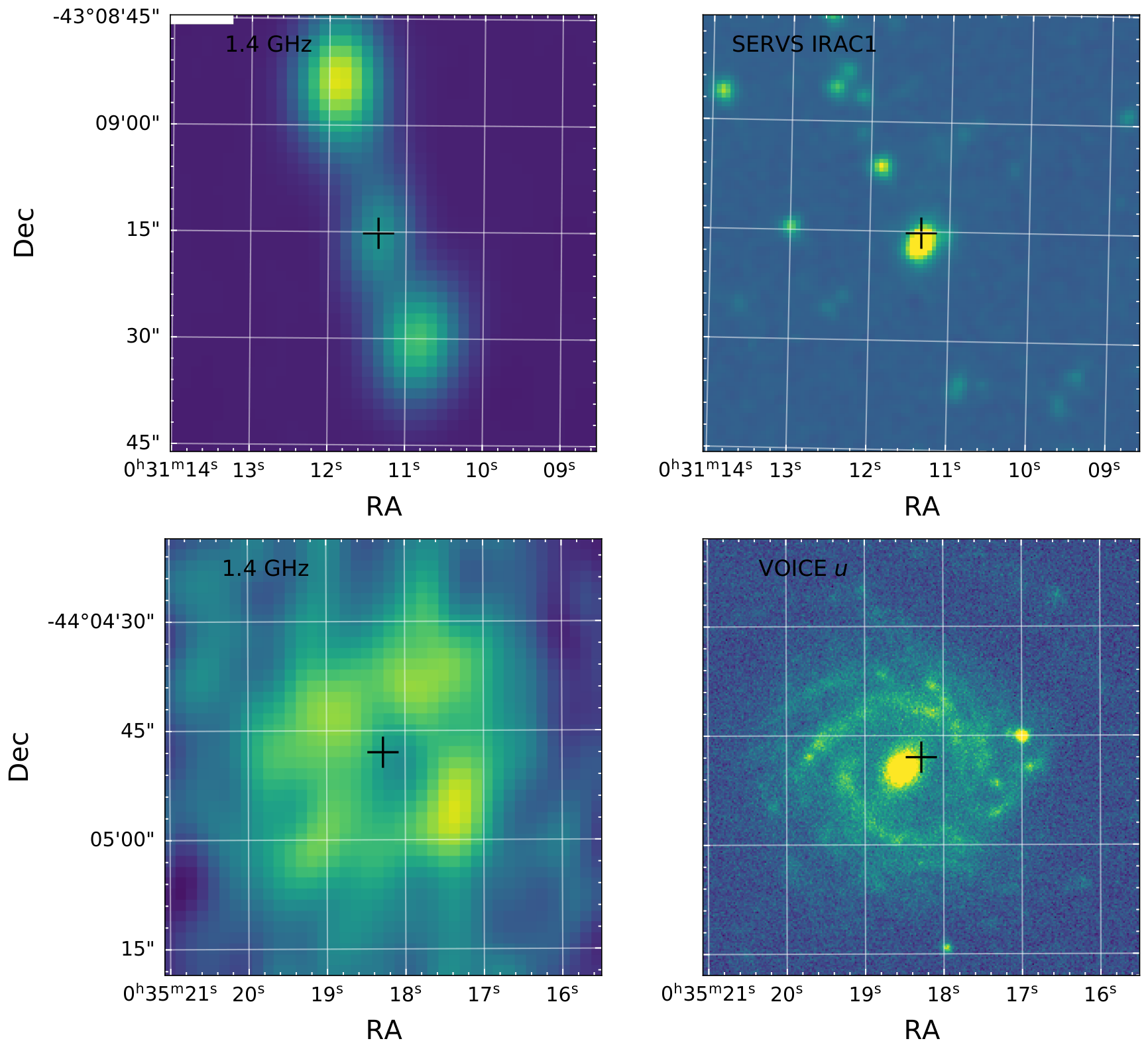
The automatic cross-matching method in the previous subsections is designed for radio sources with single components that are co-spatial with their optical/IR counterparts, which do not include the jet and lobe emission of radio galaxies. We perform visual inspection to identify radio sources with multiple sub-components and find their host galaxies. Since these sub-components do not have counterparts in the optical/IR catalogs and are often not point radio sources, we select radio sources that are flagged unmatched in § 3.3.1 and/or are flagged as resolved for visual inspection.
For each radio source, we created cutouts with an initial size of 1 1 arcmin2 in the bands of radio, VIDEO , SERVS IRAC1, and DES . When there are multiple radio images of different resolutions available, we use all radio images. For example, since the MIGHTEE/XMM-LSS field is completely within the VLA/XMM-LSS field, for each MIGHTEE source for inspection, we create three radio cutouts from the MIGHTEE high-sensitivity/low-resolution image (8.2 arcsec), the MIGHTEE low-sensitivity/high-resolution image (5 arcsec), and the VLA image (4.5 arcsec). If the initial cutouts are too small to include all radio components associated with a radio galaxy, we increase the cutout size during inspection.
In the top panels of Fig. 6, we show an example of a radio galaxy with a lobe-core-lobe morphology found by our visual inspection. In addition to AGNs, star-forming processes in very nearby galaxies also produce resolved radio sources and radio sources with multiple sub-components. The bottom panels show one case where the extended radio emission is apparently associated with a star-forming spiral disk instead of the nucleus of a galaxy.
During inspection, we also flagged those radio sources that appear confused and have multiple optical/IR counterparts. The flags are contained in Table 9. These confused radio sources are removed from the analyses in the rest of this paper. It is easiest to find confused radio sources in the MIGHTEE/XMM-LSS catalog thanks to the high-resolution image.
Point (unresolved) sources that have counterparts found in § 3.3.1 are not visually inspected. Source confusion is not expected to be significant for such radio sources since the criterion of ensures that the MLRC dominates the likelihood ratio (see Appendix A).
We provide the final cross-matching results in Table 3 and Table 4, merging the results from visual inspection and the automatic method. The radio sources appeared confused are excluded. In total, counterparts are found for 2915/3034, 1855/2084, 5462/5762, and 18974/20274 radio sources in the ATLAS/W-CDF-S, ATLAS/ELAIS-S1, VLA/XMM-LSS, and MIGHTEE/XMM-LSS surveys. In Table 4, we have combined the results of the MIGHTEE and VLA surveys in the XMM-LSS field.
[b] Name ATLASID TRACTORID VIS EXT arcmin (1) (2) (3) (4) (5) J032553.86280455.0 CI0001 99 0 99 J032554.05284155.1 CI0002 99 0 99 J032555.30283744.5 CI0003 99 0 99 J032557.32280308.9 CI0004 99 0 99 J032558.27281152.3 CI0005 99 0 99
[b] Name MTID VLAID TRACTORID VIS EXT arcmin (1) (2) (3) (4) (5) (6) J021401.02043245.4 99 J021400.99043244.3 99 0 99 J021401.24042924.3 99 J021401.36042923.3 99 0 99 J021408.85051844.3 99 J021408.85051843.9 99 1 99 J021415.46043039.4 99 J021415.45043038.4 99 1 99 J021415.65044137.0 99 J021415.65044136.0 99 1 99
[b] Step W-CDF-S ELAIS-S1 XMM-LSS Cross-matching 2762 1851 18261 VIDEO Coverage 2421 1057 17115 Bright Star Mask 2408 1051 17036 Remove Stars 2380 1041 16985
[b] Field Name -type Radio AGN X-ray AGN MIR AGN mJy mJy mJy mJy (1) (2) (3) (4) (5) (6) (7) (8) (9) (10) (11) (12) (13) W-CDF-S J032646.45284952.7 0.853 phot 0.762 0.903 000 1 0 0.333 0.041 0.8098 0.0149 W-CDF-S J032647.93283142.0 0.967 phot 0.862 1.058 001 1 0 0.631 0.040 0.0597 0.0165 W-CDF-S J032648.14284329.9 0.781 phot 0.668 0.905 001 1 0 0.297 0.034 0.0878 0.0145 W-CDF-S J032648.20275747.2 1.152 phot 1.034 1.163 001 1 0 0.895 0.049 0.2128 0.0175 W-CDF-S J032648.36280003.8 1.705 phot 1.629 1.979 001 1 0 0.180 0.021 0.0768 0.0196 SFRgal SFRagn yr-1 yr-1 (14) (15) (16) (17) (18) (19) (20) 99.4 17.9 7.3 50.7 26.8 7.9 18 112.4 0.90 0.90 154.4 0.21 0.79 11 164.7 0.17 0.31 145.3 0.13 0.40 10 6.2 67.3 2.0 6.9 39.1 2.2 10 166.7 2.0 1.0 154.9 0.89 0.94 8


3.5 Radio observations at higher and lower frequencies
We also find the counterparts of our radio sources in catalogs at higher and lower radio frequencies in the three XMM-SERVS fields. These radio surveys include the 2.3 GHz observations of the two ATLAS fields (Zinn et al. 2012), The Rapid ASKAP Continuum Survey (RACS; McConnell et al. 2020) at 887.5 MHz that covers all three XMM-SERVS fields, and the LOFAR observations at 150 MHz of the XMM-LSS field (Hale et al. 2019).
The 2.3 GHz sources in the W-CDF-S and ELAIS-S1 fields have been matched to 1.4 GHz sources in the previous data release of ATLAS. To link these 2.3 GHz sources with 1.4 GHz sources from the ATLAS DR3, we adopted a NN method with a distance cut of 5 arcsec, which results in 278 and 349 matches in the W-CDF-S and ELAIS-S1 fields, respectively.
We utilize the component-fitting results in the RACS and LOFAR catalogs to link them to the ATLAS/VLA/MIGHTEE surveys. Specifically, we find ATLAS/VLA/MIGHTEE sources that are enclosed by the ellipse defined by major axes, minor axes, and the position angle of a component in the RACS/LOFAR catalog. If only one ATLAS/VLA/MIGHTEE source is enclosed by the ellipse, we link it with the corresponding RACS/LOFAR component. If more than one ATLAS/VLA/MIGHTEE source is enclosed by the ellipse and these ATLAS/VLA/MIGHTEE sources have one unique optical/IR counterpart, we also link these ATLAS/VLA/MIGHTEE sources with the corresponding RACS/LOFAR component. Otherwise, if more than one ATLAS/VLA/MIGHTEE source is enclosed by the ellipse and these ATLAS/VLA/MIGHTEE sources have different optical/IR counterparts (including unknown optical/IR counterparts), we treat the RACS/LOFAR component as confused and remove it. In total, we matched 382/190/323 RACS sources in the W-CDF-S/ELAIS-S1/XMM-LSS fields and 751 LOFAR sources in the XMM-LSS field.
4 Multiwavelength properties of radio sources
4.1 The main sample
We define our main sample in the following way. We require the optical/IR positions of the radio sources to be covered by the VIDEO survey since the VIDEO fields have the richest multiwavelength coverage. An object is considered covered if the value on the VIDEO confidence map is larger than the 5th percentile of all positive values. Furthermore, we remove radio sources that are in the regions masked around bright stars. Finally, we match the optical/IR counterparts with the stars compiled by Zou et al. 2022 and remove these radio stars since we are most interested in extragalactic radio sources. In total, we removed 93 radio stars. The results are shown in Table 5. The sky areas of the main sample are 3.22, 1.56, and 2.96 deg2 in the W-CDF-S, ELAIS-S1, and XMM-LSS fields, leading to a total solid-angle coverage of 7.74 deg2. In comparison, the sky areas of the VIDEO data of the three fields are 4.5, 3, and 4.5 deg2, respectively; therefore, about 65% of the VIDEO fields are covered by the main radio catalog.
4.2 Redshifts
We use spectroscopic and high-quality UV-to-MIR photometric redshifts compiled by Zou et al. 2022. There are 2324/2380, 1031/1041, and 16637/16985 objects that have redshift measurements in the W-CDF-S, ELAIS-S1, and XMM-LSS fields, respectively. The fractions of spectroscopic redshifts are 42.3%, 51.2%, and 27.5%, respectively. About 75% of the photometric redshifts have quality (good photometric redshifts). In Fig. 7, we show radio sources with redshift measurements in the - plane, where is the rest-frame 5 GHz luminosity. Since only a small portion of the radio sources have multiwavelength radio data, a uniform radio spectral index of (e.g. Smolčić et al. 2017a) is adopted when we calculate .
4.3 Photometry from the X-rays to IR
We use X-ray data from the XMM-SERVS survey (Chen et al. 2018; Ni et al. 2021) to constrain the high-energy properties of the radio sources. First, we define X-ray coverage to be if the hosts of radio sources have th percentile of full-band exposure time in each field. Second, since the X-ray sources in the XMM-SERVS catalogs have been matched to their optical/IR counterparts, we link the X-ray and radio sources if their respective optical/IR positions are separated by arcsec and the X-ray position is arcsec away from the optical/IR position of the radio source. Since the median X-ray positional error is 1.2 arcsec, the 3 arcsec cut ensures that the optical/IR position is 2.5 from the X-ray position. If the X-ray position alone is arcsec from the optical/IR position of the radio source, we also think the X-ray is associated with the radio sources. This matching procedure results in 220/2285, 88/1018, and 965/16481 securely X-ray detected radio-source host galaxies that are covered by the XMM-Newton observations. Note that the X-ray detection fractions of the host galaxies of these faint radio sources are low, in the range of 5–10%. Aside from these securely X-ray detected sources, we also label sources that are securely X-ray undetected. We masked out detected X-ray sources utilizing the XMM-SERVS catalog with circular regions with a radius of arcsec, where is the full-band net counts. Generally, 10–104, rendering masks of the size of 10–40 arcsec. These masks are large enough such that the brightness of the source is below that of background beyond these radii (Read et al. 2011). The host galaxies of radio sources that are covered by X-ray observations but in the source-free regions are securely undetected, and there are 1753/2285, 814/1018, and 13193/16481 such objects in the W-CDF-S/ELAIS-S1/XMM-LSS fields. Their X-ray properties are constrained later via stacking analyses in § 4.6.
For the multiwavelength data in the optical and NIR, we mainly use the Tractor catalogs (Zou et al. 2021; Nyland et al. 2023), which cover through IRAC2. In the main samples, 2326/2380, 1031/1041, and 16644/16985 objects have counterparts in the Tractor catalogs of the W-CDF-S, ELAIS-S1, and XMM-LSS fields. The Tractor fluxes have an offset of mag compared with the original VIDEO catalog (Nyland et al. 2017) in the and bands, and we corrected these two bands with mag and mag in all three fields (cf. Table 3 of Nyland et al. 2017). Furthermore, we also find a notable offset for the CFHT band of the XMM-LSS field by comparing with the original catalog (Hudelot et al. 2012), and we correct this band by mag, which is the median offset. We find that the offsets are (sometimes) different for point sources and extended sources. Therefore, improving the PSFs used by the Tractor might help to resolve the offsets. The corrections we make are also backed by the cigale fitting results (see § 5.1). If the uncorrected fluxes are used, the distributions of the SED fit residuals at these bands are not centered around zero. Note that inconsistencies of similar magnitude between photometric catalogues derived from different techniques are also present in other fields (e.g. Davies et al. 2021). We supplement these data with the DES DR2 () photometry if the Tractor photometry is missing.
For the two red IRAC channels (5.8 and 8.0 ), we use the photometry from the Spitzer Data Fusion (Vaccari 2015). Furthermore, to construct a uniform data set in the MIR, we additionally estimate the 5.8 m and 8.0 m band upper limits from the SWIRE survey in Appendix C. Additionally, we use the WISE-3 (12) photometry from the AllWISE catalog (Wright et al. 2010), and we use a zero point of 29.045 Jy to convert the WISE-3 magnitudes to energy flux densities (Wright et al. 2010). Finally, we use MIPS 24, PACS 100, PACS 160, SPIRE 250, SPIRE 350, and SPIRE 500 photometry from the HELP project (Shirley et al. 2021), which uses the XID+ algorithm to deblend confused far-infrared (FIR) sources.55 5 We fixed issues with the XID+MIPS24 and XID+PACS catalogs in Appendix D. Note we also utilize the measurements of the upper limits (from Appendix C or Zou et al. 2022) in these FIR bands if they are not matched in the catalogs above.
4.4 Radio-Selected AGNs
The radio emission from extragalactic sources could be produced by AGN jets and/or star-forming processes. However, star-formation related radio emission is produced within the galaxy, has a typical radio spectral index of to , and is related the FIR emission (e.g. Condon 1992; Delhaize et al. 2017; Tabatabaei et al. 2017; An et al. 2021). Therefore, we select radio(-loud) AGNs using radio morphology (lobe/jet structures), radio spectral index (), or radio excess (sources with a radio excess have radio flux densities 10 or more times larger than those predicted by the parameter of Appleton et al. 2004), where . The results are given in Table 6 and also shown in the left panels of Fig. 8. There are 713, 275, and 827 radio AGNs in the W-CDF-S, ELAIS-S1, and XMM-LSS, respectively. Note that the sky density of the MIGHTEE sources in the XMM-LSS field is a factor of higher than that of the ATLAS sources in the W-CDF-S and ELAIS-S1 fields, but the sky density of radio AGNs for the former is only about 50% higher than for the latter. Therefore, as expected, radio sources fainter than the ATLAS sensitivity are dominated by galaxies and radio-quiet AGNs. The faint radio AGNs below the ATLAS sensitivity are generally harder to identify and study in detail than the objects we select in this subsection.
Note that the values we calculated are observed values (e.g. Middelberg et al. 2008), and no correction was applied, which depends upon redshift and the radio and MIR SEDs of the object. The reliability of the AGNs selected by strong radio excess is not affected by the correction. We assume a power-law spectral index of in the radio band (e.g. Bonzini et al. 2013), and an M82-like SED (e.g. Polletta et al. 2007; Ibar et al. 2008) in the MIR band. We convolve the M82 SED with the MIPS 24 m filter and normalize to 1 (Appleton et al. 2004) at zero redshift. Then, we calculate the correction of at different redshifts. The -corrected for radio-excess AGNs is shown in Fig. 9, where the dashed lines represent the range of the -corrected parameter (Appleton et al. 2004). Fig. 9 shows that these AGNs show radio excesses at a level after the correction of a star-forming galaxy, M82. The SEDs of radio AGNs might show a large diversity (see the left panel of Fig. 17). We therefore do not perform correction on the parameter here. The -corrected parameter, , is utilized in § 5.1. Furthermore, Fig. 9 indicates that we might miss some radio-excess AGNs at .
In the right panels of Fig. 8, we show MIR and X-ray AGNs among the radio sources. Most of these radio-detected MIR and X-ray AGNs are not radio-loud. Note that large-scale lobes/jets are often luminous radio emitters, and sources with measured spectral index in the radio band are also biased toward bright sources. Therefore, radio morphology/spectrum selected AGNs are almost always selected by the criterion as well. We have created the Venn diagrams of radio AGNs selected using different methods in Fig. 10.


4.5 AGNs selected in other bands
We compare radio AGNs with those selected in the X-ray and MIR in IRAC color-color space in Fig. 11. We list the number of X-ray and MIR AGNs among the radio sources in Table 7. In Fig. 11, radio AGNs do not overlap substantially with X-ray and MIR AGNs, which is consistent with the findings in Whittam et al. 2022; it is important to select AGNs using multiwavelength data. Note that we have identified 1656 new radio AGNs in these fields not found by the X-ray or MIR selection approaches. In Fig. 12, we show a Venn diagram for AGNs selected using different methods in the 7.74 deg2 region from which we selected our main sample. The sky density of radio AGNs is deg-2, which is 0.74 of that of MIR AGNs and 0.35 that of X-ray AGNs.
We also compare our radio AGNs against the CDF-S 7-Ms catalog (Luo et al. 2017), which has achieved an unmatched sky density of reliable AGNs (23900 deg-2). The deep Chandra observations cover an area of about 484 arcmin2, and we only focused on half of the area that has the top 50% of exposure time. There are 42 ATLAS radio sources within this sky region, 36 of which are matched to the CDF-S 7-Ms catalog, in which 24 and 12 objects are classified as AGNs and galaxies (see § 4.5 of Luo et al. 2017), respectively. On the one hand, we selected 16/42 objects as radio AGNs, of which only 7 are classified as AGNs in the CDF-S 7-Ms catalog. Inspecting the high-resolution VLA images (Miller et al. 2013) of the remaining 9 radio AGNs, we found in one case the ATLAS radio source is affected by source confusion and is associated with four VLA components. However, the brightest VLA source among the four still shows a radio excess and would be selected as an AGN. Therefore, the number of radio AGNs not selected by the CDF-S 7-Ms catalog is not affected. There are two radio AGNs that can be selected by their radio morphologies (note that they are also selected as RL AGNs using the criterion), both of which are detected in the Chandra 7-Ms observations but were classified as galaxies. These two radio AGNs are not MIR AGNs either. Even the deepest X-ray survey missed a substantial fraction of radio-selected AGNs. On the other hand, there are a large number of X-ray AGNs/galaxies that are not detected in the radio band. We show in Fig. 13 the Venn diagrams that compare the AGN classification of the radio sources with those objects in the Chandra catalog. Furthermore, we performed stacking analyses for the 4 objects that are classified as radio AGNs but not detected in the CDF-S 7-Ms catalog, and central point X-ray sources cannot be found in the stacked images for the non-detections.
4.6 Stacked X-ray properties

For the (X-ray undetected) objects in the source-free regions (see § 4.3), we performed stacking analyses to constrain their basic X-ray properties. Note that the median full-band exposure times (combining the pn, MOS1, and MOS2 cameras) of these objects are 89/87/100 ks in the W-CDF-S/ELAIS-S1/XMM-LSS fields. Since the sensitivity improves with for XMM-Newton observations with such exposures, we jointly analyze the X-ray data of the three fields since they have comparable depths. Utilizing the science images in the soft (0.5–2 keV), hard (2–10 keV), and full (0.5–10 keV) bands, we calculate the number of counts in the pixels (i.e. arcsec2) centered on the host positions. We estimated the background level using the median counts number for the 16 equal-size (i.e. pixels) regions surrounding the pixels centered on the host positions. In the top panel of Fig 14, we show the correlation between the full-band net counts of the X-ray undetected RL AGNs and their radio flux densities. The X-ray and radio fluxes show a weak positive correlation. The median net counts in the mJy (1624 objects), 1 mJy10 mJy (272 objects), and 10 mJy (47 objects) bins are 2.5, 5, and 10; the X-ray flux increases by a factor of 4 typically while the radio flux increases by a factor of . The sub-linear correlation in Fig. 14 (top) is consistent with previous correlation analyses for RL-AGNs and radio-loud quasars (e.g. Brinkmann et al. 2000; Miller et al. 2011; Zhu et al. 2020). In comparison, the X-ray and radio emission are almost linearly correlated for RQ-AGNs and radio-quiet quasars (e.g. Brinkmann et al. 2000; Laor & Behar 2008). The 25th, 50th, and 75th percentiles of the corresponding net counts of the X-ray detected RL AGNs are 35.8, 65.8, and 141.7, respectively. Therefore, the X-ray undetected objects are typically times fainter than those of the detected objects.
We also calculate the hardness ratio to assess if the spectra of X-ray undetected RL AGNs are different from those of detected objects. We define hardness ratio , where and are the net counts in the hard and soft bands, respectively. We stacked the hard-band and soft-band net counts in the three radio-flux bins and calculated corresponding hardness ratios. The results are shown in the bottom panel of Fig. 14, where the errors are estimated using bootstrapping. For comparison, we also show the HR distribution of the X-ray detected RL AGNs. The average HRs in the three flux bins are not significantly different from those of the detected objects, suggesting that their X-ray faintness is not mainly due to additional obscuration.
[b] Radio AGNs W-CDF-S ELAIS-S1 XMM-LSS Total 713 275 827 X-ray Detections 66 28 62 X-ray AGNs 65 20 62 Donley MIR AGNs 19 4 19 Radio-Onlya 641 254 761
- a
Radio-only refers to radio AGNs that are neither X-ray AGNs nor Donley et al. 2012 MIR AGNs.


[b] Module Paramter Value galaxy-only model dale2014 alpha 1.0, 1.25, 1.5, 1.75, 2.0, 2.25, 2.5, 2.75, 3.0 dustatt_modified_starburst E_BV_lines 0.0001, 0.001, 0.01, 0.02, 0.04, 0.06, 0.08, 0.1, 0.15, 0.2, 0.3, 0.4, 0.5, 0.6, 0.8, 1, 1.2 radio qir_sf 2.34 R_agn 0.0 galaxy+AGN model dale2014 alpha 1.0, 2.0, 3.0 dustatt_modified_starburst E_BV_lines 0.001, 0.01, 0.1, 0.2, 0.3, 0.4, 0.5, 0.6, 0.8, 1, 1.2 skirtor2016 t 3, 7, 11 i 0, 10, 30, 50, 70, 90 fracAGN 0.1, 0.2, 0.4, 0.6, 0.8, 0.99
5 Discussion
5.1 The SEDs of faint radio sources
We constrain the SEDs of the radio sources utilizing cigale (v2022.1, Boquien et al. 2019; Yang et al. 2020; Yang et al. 2022), from which we estimate the stellar masses, star-formation rates, and other physical parameters of the host galaxies. Zou et al. 2022 fit the SEDs of millions of objects in the three DDFs we have studied in this paper. Our fitting methods generally follow those of Zou et al. 2022 but with some modifications. First, the photometric data are summarized in Table 1 of Zou et al. 2022. We use a similar data set with the addition of the WISE-3 band (m; see § 4.3), which fills the gap between the IRAC m and MIPS m bands. Furthermore, we exclude the X-ray data from the fitting. Only a small fraction of the radio sources have detected X-ray counterparts; excluding the X-ray band reduces the required computation by a large factor. Secondly, each object might have multiple optical fluxes in similar filters, and Zou et al. 2022 use all available photometric data in the fitting. We select only the “best” fluxes in the order of HSC, VOICE, VIDEO, CFHTLS, and DES. If a higher order flux is available for one of the bands, the remaining fluxes in the same band are ignored. Thirdly, we utilize the radio module of cigale to predict the radio emission that is produced by star formation. In the radio module, qir_sf represents the parameter (Helou et al. 1985),
| (6) |
where is the rest-frame FIR flux that is estimated from the IRAS 60 and 100 m fluxes, and the flux at rest-frame 1.4 GHz. is similar to the parameter but uses longer-wavelength FIR fluxes that trace the star-forming processes better. Furthermore, is defined for rest-frame quantities, and the correction is avoided using the best-fit cigale models. The radio module has a parameter R_agn that represents the radio-loudness parameter of AGNs, (Yang et al. 2022), where and are the monochromatic luminosities at rest-frame 5 GHz and 2500 Å, respectively. We fix qir_sf (e.g. Yun et al. 2001) and R_agn in the parameter settings.66 6 The values of from previous studies are generally in the range of 2–2.41 (cf. Sargent et al. 2010). Delvecchio et al. 2021 report a value of about 2.6 and find that might depend strongly on stellar mass and mildly on redshift, probably because the radio data (VLA 3GHz observations in the COSMOS field) they use have a smaller beam size and are at a higher frequency than previous studies. Note that the radio band is not included in the fitting; the radio module simply calculates the radio fluxes at 1.4 GHz that are expected to be produced by star formation, which are not compared with the observed fluxes in the fitting process.
Following Zou et al. 2022, the SED of each object is fit twice, once with a galaxy-only model and once with a galaxy+AGN model, the parameter settings of which are similar to those in Table 4 and Table 5 of Zou et al. 2022, respectively. In Table 8, we give the few parameters that are different from those in Zou et al. 2022. It is a common practice to add systematic uncertainties to the flux-density errors in cigale. However, we find this practice unnecessary (cf. Fig. 16) for our datasets in part because an additional 3%–9% flux uncertainty has been added on top of the statistical uncertainties (in quadrature) in the Tractor photometry catalogues (K. Nyland 2023, private communication). We turn this feature off by setting additionalerror=0 (the default value is 10%). In Fig. 15, we compare the statistic of the best-fit galaxy-only model with that of the best-fit galaxy+AGN model.77 7 In Zou et al. 2022, different best-fit models are compared using BIC, which is equal to , where is the number of fluxes. Radio AGNs we selected in § 4.4 and AGNs that are selected using MIR/X-ray methods are represented by different symbols. Since the parameter settings of the galaxy+AGN model are less dense than those of the galaxy-only model (Zou et al. 2022), the latter is not a special case of the former with zero AGN component. Otherwise, would always be true. Notably, the majority of the MIR/X-ray AGNs prefer the galaxy+AGN model with , while radio AGNs generally prefer the galaxy-only model, indicating that the signatures of active nuclei are not strong for these AGNs at bands other than the radio. The host-galaxy property (stellar mass and SFR) results from the cigale fits are provided in Table 6. For each object, we use the fitting results with the smaller between those of the galaxy-only and galaxy+AGN models.
We show typical SED fitting results for radio AGNs in Fig. 16. For each field, we separate the objects that prefer the galaxy-only and galaxy+AGN models, and choose the object with the median reduced (i.e. ) in each group. Note that cigale counts the number of data points including upper limits when calculating the degrees of freedom. We recalculate the reduced including only the detected fluxes. Generally, the cigale models reproduce well the observed fluxes from the UV-to-FIR bands. The median reduced in Fig. 16 are close to unity. We acknowledge that the Spitzer/PACS and Herschel/SPIRE data points are very often upper limits, and the FIR band is effectively constrained only by the MIPS 24 Jy fluxes and UV/optical fluxes via the energy-balance principle of cigale (Boquien et al. 2019; Yang et al. 2020).
We show the best-fit SEDs from 100 nm to 1000 m of radio AGNs and MIR/X-ray AGNs in the left and right panels of Fig. 17, respectively. Even though the two populations do not substantially overlap (see Fig. 12), we exclude objects that are both radio and MIR/X-ray AGNs in Fig. 17. Therefore, the radio AGNs here refer to the AGNs that are only selected in the radio band but not with other methods. Furthermore, we exclude objects with to remove low-quality fits so that the model-dependent cigale SEDs well depict the underlying true SEDs. The SEDs of the remaining objects are first normalized to following Zou et al. 2022. Then, the SEDs are rebinned in rest-frame wavelength from 1000 m to 100 nm with a bin size of 0.02 dex. We calculate the composite median SEDs for the radio and MIR/X-ray AGNs and plot them in both panels of Fig. 17. The SEDs of typical radio AGNs show two prominent peaks in the optical/NIR and FIR bands, while those of the MIR/X-ray AGNs are flatter and show excess emission in the UV and MIR bands. The contrast between the stacked SEDs of radio AGNs and MIR/X-ray AGNs is consistent with Fig. 12 where radio AGNs overlap little with AGNs selected using MIR/X-ray methods, probably because a substantial fraction of the radio AGNs we select are low-luminosity radio galaxies without bright and blue accretion disks and hot, dusty tori. Notably, the radio AGNs seem to contain a small but substantial population of objects that are dust-poor.
In Fig. 18, we compare the radio emission that is related to star formation in the host galaxies with the observed total radio fluxes. The radio AGNs selected using the parameter are generally consistent with the parameter. Furthermore, a larger value of (see Footnote 6) will shift the data points downward by dex and move radio-excess AGNs further away from the black line. Most of the remaining, probably star formation-dominated, objects seem consistent with and seem unlikely to tolerate a vertical shift of dex. At radio fluxes below 0.1 mJy, the parameter shows a population of radio-excess AGNs that are missed by the parameter due to the limited sensitivity of the 24m data.
We show the “Bayesian-like” estimations of SFR and stellar mass from cigale fits in Fig. 19. The host galaxies of radio AGNs are generally more massive than those of MIR/X-ray AGNs. The SFRs of radio AGNs can reach as high as those of MIR/X-ray AGNs. However, a large fraction of radio AGNs have SFR yr-1.
We further split the radio AGNs into six redshift bins from to 2.7 with a bin width of 0.4 and show the results in Fig. 20. We compare radio AGNs with the “main sequence” of Popesso et al. 2022 in each redshift bin. The SFR and for the VIDEO-selected galaxies in the three DDFs from Zou et al. 2022 are shown as small grey points in Fig. 20, which are consistent with the main sequence of Popesso et al. 2022 except for the first bin (i.e. the top-left panel of Fig. 20). We also plot the main sequence of Leja et al. 2022 in the first redshift bin in green, which is more consistent with the star-forming galaxies of Zou et al. 2022. A progressively larger fraction of radio AGNs are hosted by main-sequence galaxies with increasing redshift; while most radio AGNs live in massive, quiescent galaxies at , star-forming galaxies dominate the host galaxies of radio AGNs at –2.7, where the cosmic star formation peaks. Note that our paper and Zou et al. 2022 use similar data sets and methods to derive the SFR and stellar mass, and our results are not affected by the definition of the main sequence from the literature. The main sequences of Popesso et al. 2022 and Leja et al. 2022 in Fig. 20 are only used to guide visualization. The large orange points in Fig. 20 show the radio AGNs that are also X-ray and/or MIR AGNs. These objects are high-excitation radio galaxies (HERGs), and most of the large blue points are likely low-excitation radio galaxies (LERGs) because LERGs show little sign of active nuclei except in the radio band. Using the MIGHTEE/COSMOS data, Whittam et al. 2022 find that HERGs and LERGs show little difference in SFR and stellar mass, which is in contrast with the results in the local universe. Our results seem consistent with those of Whittam et al. 2022 in that there is no apparent difference between the host-galaxy SFRs and stellar masses of HERGs and LERGs at high redshift.


5.2 The dependence of the incidence of radio AGNs on galaxy stellar mass and redshift
We investigate how the properties of the galaxies (and redshift) could affect the incidence of radio AGNs using the SED fitting results of this paper and Zou et al. 2022. We select the galaxy sample from Zou et al. 2022 as in § 4.1 and focus on galaxies with and . Given the depth of the VIDEO survey, the sample is complete for galaxies up to . The galaxies are split into - bins with a step of 0.4 in redshift and a step of 0.3 dex in stellar mass. The fraction of radio AGNs in each bin is calculated. The errors of the radio AGN fraction are calculated using astropy.stats.binom_conf_interval with the flat method (e.g. Cameron 2011). The results are shown in the top panel of Fig. 21. The dependence of the radio AGN fraction on stellar mass is strong such that the fraction increases by 2–3 orders of magnitude from to . However, the stellar-mass dependence in the bins is not as strong as in the bins.
In the bottom panel of Fig. 21, we show the dependence of radio AGN fraction upon SFR. The overall shape of the relation is consistent with a “V” shape throughout the redshift range we study, indicating that the fraction of radio AGNs first decreases and then increases with SFR. The SFR and the radio-AGN fraction at the vertex of the “V” both increase with redshift. The bottom panel of Fig. 21 is consistent with a scenario where the radio AGNs could be hosted by both quiescent and star-forming galaxies, and the incidence of radio AGNs decreases with SFR in quiescent galaxies but increases with SFR in star-forming galaxies. The triggering mechanism of radio AGNs might thus be different in quiescent galaxies and star-forming galaxies. Furthermore, there are overall increases of SFR and radio AGN fraction for all types of galaxies from to –3, shifting the vertex of the “V”.
Thanks to the deep multiwavelength coverage in the three DDFs we study in this paper, the incidence rate of radio AGNs has been constrained to a higher redshift than in previous work (e.g. Kondapally et al. 2022). The incidence of X-ray selected AGNs also increases with stellar mass. A strong positive evolution with redshift is found for X-ray AGNs with (e.g. Yang et al. 2018; Aird et al. 2019), which is consistent with radio AGNs in the first two stellar-mass bins of the top panel of Fig. 21. However, for the most massive galaxies with , the radio AGN fraction decreases with redshift. Furthermore, the X-ray AGN fraction increases almost linearly with the SFR (e.g. Aird et al. 2019), which is not the case for radio AGNs, probably because most radio AGNs are hosted by quiescent galaxies and fueled by the cooling of hot gas.


6 Summary and Future Prospects
6.1 Summary of main results
We have performed deep radio AGN selection and characterization in three well-studied multiwavelength survey fields (W-CDF-S, ELAIS-S1, and XMM-LSS) spanning 11.3 deg2 in total that will soon be extensively observed by Rubin as DDFs. The deep radio data used are from the ATLAS/W-CDF-S, ATLAS/ELAIS-S1, VLA/XMM-LSS, and MIGHTEE/XMM-LSS surveys. Our main results are the following:
1. We have performed careful cross-matching of the 25,000 faint radio sources to optical, NIR, and MIR objects that has successfully identified reliable counterparts for most (93–96%) of the radio sources; such counterparts are essential for AGN selection and characterization. See §2 and §3.
2. We have constructed FIR-to-X-ray SEDs for the counterparts of the 22,000 radio sources in our main (7.7 deg2) sample. About 82% of these radio sources have spectroscopic or high-quality photometric redshifts available, and these indicate that most of the radio sources lie at . See §4.2 and §4.3.
3. We have selected 1815 radio AGNs in our three fields based upon radio morphology (lobe/jet structures), radio spectral index (), and excess radio flux () criteria. As expected from other surveys, these radio AGNs usually do not overlap with AGNs selected using X-ray and MIR techniques. In fact, 1656 of the 1815 radio AGNs (91%) had not been identified as AGNs previously based upon their X-ray and/or MIR emission. This represents a substantive increase of the total AGN population in these key sky fields. See §4.4 and §4.5.
4. Stacking of the sensitive XMM-SERVS X-ray data in these fields shows only a weak positive correlation between the X-ray and radio fluxes, and the average X-ray hardness ratios of the X-ray detected and X-ray undetected radio AGNs are statistically consistent. See §4.6.
5. We have fit the FIR-to-UV SEDs of all radio sources using cigale from which we derive, e.g., host-galaxy stellar masses and star-formation rates. As expected, most radio AGNs prefer galaxy-only SED models statistically, indicating that AGN signatures for such sources are generally weak at bands other than the radio. See §5.1.
6. We have measured the dependence of the radio AGN fraction upon stellar mass and SFR out to . The fraction strongly rises with stellar mass, although this rise is weaker at higher redshifts. The dependence of radio AGN fraction appears to decrease with SFR in quiescent galaxies and increase with SFR in star-forming galaxies. See § 5.2.
6.2 Future work
The 1815 radio AGNs selected in this work will be studied extensively over the next decade by multiple facilities. Rubin, Euclid, the Roman Space Telescope, and the Hawaii Two-0 Survey, for example, will obtain superb NIR-to-optical photometric and imaging data that will further constrain their photometric redshifts, SEDs, and morphologies. The resulting measurements of stellar masses, star-formation rates, and host-galaxy structures will shed light on the triggering mechanisms for radio AGNs to high redshift. Some of these photometric data will also allow time-domain studies, although many of the radio AGNs have host-dominated SEDs outside the radio band so are not expected to show strong NIR-to-optical variability. Our radio AGNs will also be extensively targeted by powerful spectroscopic surveys, including the Deep Extragalactic Visible Legacy Survey (DEVILS), the Multi-Object Optical and Near-Infrared Spectrograph (MOONS) survey, the Subaru Prime Focus Spectrograph (PFS) survey, and the Wide Area VISTA Extragalactic Survey (WAVES). These will provide precise redshifts as well as further characterize the nature of our sources spectroscopically. The precise redshifts will allow our radio AGNs to be placed in their large-scale cosmic environmental context; such radio AGNs often trace groups and clusters. While rapid black-hole growth does not appear to depend materially upon cosmic environment once stellar mass is controlled (e.g., Yang et al. 2018; Krishnan et al. 2020), large-sample studies are still needed to assess the environmental dependence of jet-driven feedback by radio AGNs that generally represent lower accretion-rate systems in a “maintenance mode”. Ultimately, deeper X-ray coverage of the LSST DDFs by missions including Athena, STAR-X, and AXIS should detect a larger fraction of our radio AGNs, allowing their accretion properties to be clarified.
Many more radio sources in the W-CDF-S and ELAIS-S1 fields will be detected as deeper radio observations are gathered; e.g., by the MIGHTEE survey, which should raise the radio-source sky density by a factor of . Based on our results for the XMM-LSS field in §4.5, however, the increment of radio AGNs will be more modest—about a factor of 50% (the remaining majority of radio sources will be a combination of star-forming galaxies and radio-quiet AGNs). The MIGHTEE-H i project will provide a probe of the state and kinematics of neutral gas around RL AGNs via H i absorption, and the polarisation observations of MIGHTEE will provide another probe of intrinsic and environmental properties of RL AGNs.
Acknowledgements
We thank the anonymous referee and the scientific editor, Tim Pearson, for their comments that improved the clarity of our manuscript. SZ, WNB, WY, and FZ acknowledge support from NSF grant AST-2106990, NASA grant 80NSSC19K0961, Chandra X-ray Center grant AR1-22008X, and Penn State ACIS Instrument Team Contract SV4-74018 (issued by the Chandra X-ray Center, which is operated by the Smithsonian Astrophysical Observatory for and on behalf of NASA under contract NAS8-03060). B.L. acknowledges financial support from the National Natural Science Foundation of China grant 11991053. Y.Q.X. acknowledges support from NSFC grants (12025303 and 11890693), the K.C. Wong Education Foundation, and the science research grants from the China Manned Space Project with NO. CMS-CSST-2021-A06. The Chandra ACIS Team Guaranteed Time Observations (GTO) utilized were selected by the ACIS Instrument Principal Investigator, Gordon P. Garmire, currently of the Huntingdon Institute for X-ray Astronomy, LLC, which is under contract to the Smithsonian Astrophysical Observatory via Contract SV2-82024.
Data availability
The catalogues released in this article are available as online supplementary material, and they can also be downloaded at https://personal.psu.edu/wnb3/xmmservs/xmmservs.html
References
- Abbott et al. (2021) Abbott T. M. C., et al., 2021, ApJS, 255, 20
- Aird et al. (2019) Aird J., Coil A. L., Georgakakis A., 2019, MNRAS, 484, 4360
- An et al. (2021) An F., et al., 2021, MNRAS, 507, 2643
- Appleton et al. (2004) Appleton P. N., et al., 2004, ApJS, 154, 147
- Barbieri & Bertola (1972) Barbieri C., Bertola F., 1972, MNRAS, 156, 399
- Berta et al. (2006) Berta S., et al., 2006, A&A, 451, 881
- Bertin & Arnouts (1996) Bertin E., Arnouts S., 1996, A&AS, 117, 393
- Bonzini et al. (2013) Bonzini M., Padovani P., Mainieri V., Kellermann K. I., Miller N., Rosati P., Tozzi P., Vattakunnel S., 2013, MNRAS, 436, 3759
- Boquien et al. (2019) Boquien M., Burgarella D., Roehlly Y., Buat V., Ciesla L., Corre D., Inoue A. K., Salas H., 2019, A&A, 622, A103
- Bradley et al. (2020) Bradley L., et al., 2020, astropy/photutils: 1.0.0, doi:10.5281/zenodo.4044744, https://doi.org/10.5281/zenodo.4044744
- Brandt et al. (2018) Brandt W. N., et al., 2018, arXiv e-prints, p. arXiv:1811.06542
- Brinkmann et al. (2000) Brinkmann W., Laurent-Muehleisen S. A., Voges W., Siebert J., Becker R. H., Brotherton M. S., White R. L., Gregg M. D., 2000, A&A, 356, 445
- Brusa et al. (2007) Brusa M., et al., 2007, ApJS, 172, 353
- Cameron (2011) Cameron E., 2011, Publ. Astron. Soc. Australia, 28, 128
- Chang et al. (2017) Chang Y.-Y., et al., 2017, ApJS, 233, 19
- Chen et al. (2018) Chen C. T. J., et al., 2018, MNRAS, 478, 2132
- Ciliegi et al. (2003) Ciliegi P., Zamorani G., Hasinger G., Lehmann I., Szokoly G., Wilson G., 2003, A&A, 398, 901
- Condon (1992) Condon J. J., 1992, ARA&A, 30, 575
- Davies et al. (2021) Davies L. J. M., et al., 2021, MNRAS, 506, 256
- Delhaize et al. (2017) Delhaize J., et al., 2017, A&A, 602, A4
- Delvecchio et al. (2021) Delvecchio I., et al., 2021, A&A, 647, A123
- Donley et al. (2012) Donley J. L., et al., 2012, ApJ, 748, 142
- Fan et al. (2015) Fan D., Budavári T., Norris R. P., Hopkins A. M., 2015, MNRAS, 451, 1299
- Fan et al. (2020) Fan D., Budavári T., Norris R. P., Basu A., 2020, MNRAS, 498, 565
- Franzen et al. (2015) Franzen T. M. O., et al., 2015, MNRAS, 453, 4020
- Hale et al. (2019) Hale C. L., et al., 2019, A&A, 622, A4
- Hales et al. (2014) Hales C. A., et al., 2014, MNRAS, 441, 2555
- Hancock et al. (2018) Hancock P. J., Trott C. M., Hurley-Walker N., 2018, Publications of the Astronomical Society of Australia, 35, e011
- Helou et al. (1985) Helou G., Soifer B. T., Rowan-Robinson M., 1985, ApJ, 298, L7
- Herschel Point Source Catalogue Working Group et al. (2020) Herschel Point Source Catalogue Working Group et al., 2020, VizieR Online Data Catalog, p. VIII/106
- Heywood et al. (2020) Heywood I., Hale C. L., Jarvis M. J., Makhathini S., Peters J. A., Sebokolodi M. L. L., Smirnov O. M., 2020, MNRAS, 496, 3469
- Heywood et al. (2022) Heywood I., et al., 2022, MNRAS, 509, 2150
- Hickox et al. (2009) Hickox R. C., et al., 2009, ApJ, 696, 891
- Hudelot et al. (2012) Hudelot P., et al., 2012, VizieR Online Data Catalog, p. II/317
- Ibar et al. (2008) Ibar E., et al., 2008, MNRAS, 386, 953
- Ivezić et al. (2019) Ivezić Ž., et al., 2019, ApJ, 873, 111
- Jarvis et al. (2013) Jarvis M. J., et al., 2013, MNRAS, 428, 1281
- Jarvis et al. (2016) Jarvis M., et al., 2016, in MeerKAT Science: On the Pathway to the SKA. p. 6 (arXiv:1709.01901)
- Kondapally et al. (2022) Kondapally R., et al., 2022, MNRAS, 513, 3742
- Krishnan et al. (2020) Krishnan C., et al., 2020, MNRAS, 494, 1693
- Lacy et al. (2007) Lacy M., Petric A. O., Sajina A., Canalizo G., Storrie-Lombardi L. J., Armus L., Fadda D., Marleau F. R., 2007, AJ, 133, 186
- Lacy et al. (2021) Lacy M., et al., 2021, MNRAS, 501, 892
- Laor & Behar (2008) Laor A., Behar E., 2008, MNRAS, 390, 847
- Leja et al. (2022) Leja J., et al., 2022, ApJ, 936, 165
- Lonsdale et al. (2003) Lonsdale C. J., et al., 2003, PASP, 115, 897
- Luo et al. (2010) Luo B., et al., 2010, ApJS, 187, 560
- Luo et al. (2017) Luo B., et al., 2017, ApJS, 228, 2
- MIPS Instrument and MIPS Instrument Support Teams (2021) MIPS Instrument and MIPS Instrument Support Teams 2021, MIPS Instrument Handbook, doi:10.26131/IRSA488, https://catcopy.ipac.caltech.edu/dois/doi.php?id=10.26131/IRSA488
- Mao et al. (2010) Mao M. Y., Sharp R., Saikia D. J., Norris R. P., Johnston-Hollitt M., Middelberg E., Lovell J. E. J., 2010, MNRAS, 406, 2578
- Mao et al. (2012) Mao M. Y., et al., 2012, MNRAS, 426, 3334
- Marchesi et al. (2016) Marchesi S., et al., 2016, ApJ, 817, 34
- Mauduit et al. (2012) Mauduit J. C., et al., 2012, PASP, 124, 714
- McConnell et al. (2020) McConnell D., et al., 2020, Publ. Astron. Soc. Australia, 37, e048
- Middelberg et al. (2008) Middelberg E., et al., 2008, AJ, 135, 1276
- Miller et al. (2011) Miller B. P., Brandt W. N., Schneider D. P., Gibson R. R., Steffen A. T., Wu J., 2011, ApJ, 726, 20
- Miller et al. (2013) Miller N. A., et al., 2013, ApJS, 205, 13
- Nakos et al. (2009) Nakos T., et al., 2009, A&A, 494, 579
- Naylor et al. (2013) Naylor T., Broos P. S., Feigelson E. D., 2013, ApJS, 209, 30
- Ni et al. (2021) Ni Q., et al., 2021, ApJS, 256, 21
- Norris et al. (2006) Norris R. P., et al., 2006, AJ, 132, 2409
- Nyland et al. (2017) Nyland K., et al., 2017, ApJS, 230, 9
- Nyland et al. (2023) Nyland K., Lacy M., Brandt W. N., Yang G., Ni Q., Sajina A., Zou F., Vaccari M., 2023, Research Notes of the American Astronomical Society, 7, 33
- Padovani (2016) Padovani P., 2016, A&ARv, 24, 13
- Padovani et al. (2017) Padovani P., et al., 2017, A&ARv, 25, 2
- Pineau et al. (2011) Pineau F. X., Motch C., Carrera F., Della Ceca R., Derrière S., Michel L., Schwope A., Watson M. G., 2011, A&A, 527, A126
- Pineau et al. (2017) Pineau F. X., et al., 2017, A&A, 597, A89
- Polletta et al. (2007) Polletta M., et al., 2007, ApJ, 663, 81
- Popesso et al. (2022) Popesso P., et al., 2022, arXiv e-prints, p. arXiv:2203.10487
- Poulain et al. (2020) Poulain M., et al., 2020, A&A, 634, A50
- Read et al. (2011) Read A. M., Rosen S. R., Saxton R. D., Ramirez J., 2011, A&A, 534, A34
- SWIRE Project (2020) SWIRE Project 2020, The Spitzer Wide-area InfraRed Extragalactic Survey, doi:10.26131/IRSA406, https://catcopy.ipac.caltech.edu/dois/doi.php?id=10.26131/IRSA406
- Salvato et al. (2018) Salvato M., et al., 2018, MNRAS, 473, 4937
- Sargent et al. (2010) Sargent M. T., et al., 2010, ApJS, 186, 341
- Scolnic et al. (2018) Scolnic D. M., et al., 2018, arXiv e-prints, p. arXiv:1812.00516
- Shirley et al. (2019) Shirley R., et al., 2019, MNRAS, 490, 634
- Shirley et al. (2021) Shirley R., et al., 2021, MNRAS, 507, 129
- Smolčić et al. (2017a) Smolčić V., et al., 2017a, A&A, 602, A1
- Smolčić et al. (2017b) Smolčić V., et al., 2017b, A&A, 602, A2
- Spitzer Science Center and Infrared Science Archive (2020) Spitzer Science Center and Infrared Science Archive 2020, Spitzer Enhanced Imaging Products, doi:10.26131/IRSA433, https://catcopy.ipac.caltech.edu/dois/doi.php?id=10.26131/IRSA433
- Surace et al. (2005) Surace J. A., Shupe D. L., Fang F., Evans T., Alexov A., Frayer D., Lonsdale C. J., SWIRE Team 2005, in American Astronomical Society Meeting Abstracts. p. 63.01
- Sutherland & Saunders (1992) Sutherland W., Saunders W., 1992, MNRAS, 259, 413
- Tabatabaei et al. (2017) Tabatabaei F. S., et al., 2017, ApJ, 836, 185
- Tasse et al. (2008) Tasse C., Le Borgne D., Röttgering H., Best P. N., Pierre M., Rocca-Volmerange B., 2008, A&A, 490, 879
- Timlin et al. (2016) Timlin J. D., et al., 2016, ApJS, 225, 1
- Vaccari (2015) Vaccari M., 2015, in The Many Facets of Extragalactic Radio Surveys: Towards New Scientific Challenges. p. 27 (arXiv:1604.02353)
- Weston et al. (2018) Weston S. D., Seymour N., Gulyaev S., Norris R. P., Banfield J., Vaccari M., Hopkins A. M., Franzen T. M. O., 2018, MNRAS, 473, 4523
- Whittam et al. (2022) Whittam I. H., et al., 2022, MNRAS, 516, 245
- Wolf et al. (2004) Wolf C., et al., 2004, A&A, 421, 913
- Wright et al. (2010) Wright E. L., et al., 2010, AJ, 140, 1868
- Yang et al. (2018) Yang G., Brandt W. N., Darvish B., Chen C. T. J., Vito F., Alexander D. M., Bauer F. E., Trump J. R., 2018, MNRAS, 480, 1022
- Yang et al. (2020) Yang G., et al., 2020, MNRAS, 491, 740
- Yang et al. (2022) Yang G., et al., 2022, ApJ, 927, 192
- Yun et al. (2001) Yun M. S., Reddy N. A., Condon J. J., 2001, ApJ, 554, 803
- Zhu et al. (2020) Zhu S. F., Brandt W. N., Luo B., Wu J., Xue Y. Q., Yang G., 2020, MNRAS, 496, 245
- Zinn et al. (2012) Zinn P. C., Middelberg E., Norris R. P., Hales C. A., Mao M. Y., Randall K. E., 2012, A&A, 544, A38
- Zou et al. (2021) Zou F., et al., 2021, Research Notes of the American Astronomical Society, 5, 31
- Zou et al. (2022) Zou F., et al., 2022, ApJS, 262, 15
Appendix A The optimal likelihood-ratio cut
We calculate the ratio of the likelihood that the MLRC is a genuine counterpart over the likelihood that the MLRC is a confusing object,
| (7) |
In a special case where the photometric properties are ignored, the likelihood ratio is
| (8) |
which is consistent with Section 2.2 of Sutherland & Saunders 1992. The optimal that balances the number of matched genuine counterparts and the number of false positives can be found by solving .88 8 It is straightforward to solve Eq. 8 and find that the optimal distance cut for the classic NN method is . The optimal distance cut does not exist if , which is rarely the case in practice. We denote this cut , which depends upon and, therefore, upon the positional uncertainties of radio sources. Equivalently, we can use directly to screen MLRCs without finding the value of . The reliability of the MLRC is
| (9) |
and is equivalent to . Therefore, our optimal cut maximizes , where is the number of matched genuine counterparts and the number of false positives.
and are expected to be consistent since they describe the same quantity (Sutherland & Saunders 1992); the former utilizes the “nearest neighbour” and relies more on prior knowledge (i.e. and positional error and photometric distributions) while the latter utilizes all candidates and relies less on prior knowledge. As an example, we show the resulting , , and of the ATLAS-VIDEO/W-CDF-S matching in Fig. 22. Therefore, , , and corresponds (approximately) to the same optimal cut of . In practice, is not only easier to calculate but also less likely to be affected by source confusion than . For confused radio sources associated with multiple close counterparts, is easily diluted to while could still be large.
Using our optimal likelihood-ratio cut, it is straightforward to predict the completeness,
| (10) |
Then, the purity, , is predicted by calculating
| (11) |
Note that simulations are often used to assess the completeness and purity of cross-matching results in the literature. These simulations are Monte-Carlo equivalents of the integrations in Eqs. 10 and 11. However, since simulations are rarely sufficiently realistic to correct for the issues we mention in § 3.2 and, especially, Footnote 2, the estimated completeness and purity are likely not as accurate as those from Eqs. 10 and 11. The two equations above are general, and can be replaced by other cuts.

Appendix B Results of the probabilistic cross matching
In Table 9, we provide the full results of the probabilistic cross matching of § 3.3.1, which includes the reliability, , of all candidates.
[b] Radio OIR ID RA Dec RA Dec StarMask (Radio) (Radio) arcsec arcsec (OIR) (OIR) (1) (2) (3) (4) (5) (6) (7) (8) (9) (10) ATLAS/W-CDF-S DES CI0002 51.47524 28.69829 0.49 1.04 51.47522 28.69864 0 ATLAS/W-CDF-S DES CI0004 51.48881 28.05203 0.35 0.65 51.48885 28.05247 0 ATLAS/W-CDF-S DES CI0005 51.49254 28.19756 0.56 1.24 51.49310 28.19769 0 ATLAS/W-CDF-S DES CI0006 51.49392 27.42286 0.93 2.16 51.49381 27.42157 0 ATLAS/W-CDF-S DES CI0006 51.49392 27.42286 0.93 2.16 51.49492 27.42537 0 MLRC Confused (11) (12) (13) (14) (15) 6.76 0.95 1 10.58 0 9.13 0.96 1 16.64 0 0.03 0.089 1 0.083 0 0.23 0.088 0 - 0 0.00 0.000 0 - 0
Appendix C Upper limits in the IRAC 5.8 micron and 8.0 micron bands
The IR bands are important for assessing the levels of AGN and SF activity. For objects that are not detected in the two redder Spitzer/IRAC channels, we calculate their flux upper limits. We downloaded the IRAC 5.8/8.0 m science mosaics of the most recent public release of SWIRE (SWIRE Project 2020). Note that the native units of the downloaded mosaics are 1 MJy steradian-1, which can be converted to more convenient units using 1 MJy steradian Jy pixel-2 given the pixel scale of 0.6 arcsec (Timlin et al. 2016). Masks of bright stars created using the method of Mauduit et al. 2012 are always applied in the following steps. After masking out sources detected in the corresponding catalog, we estimated the background of each image using the SExtractorBackground method implemented in astropy/photutils (Bradley et al. 2020), which is then subtracted from the image. Then, to minimize the effects of the emission from detected sources on undetected sources, we remove the fluxes of detected sources from the images. We used the PSF-photometry method of photutils and set initial source positions at those of the detected sources. The IRAC point response functions (PRFs) are utilized in this procedure, after which we obtain residual images. The residual images of different tiles are combined into single images for each band (each field consists of 12–16 tiles). Then, we performed forced photometry at the positions of VIDEO sources using circular apertures of radius of 1.9 arcsec. The ‘subpixel’ method of photutils that splits each pixel into subpixels is adopted in the aperture photometry, which is consistent with that of SExtractor (Bertin & Arnouts 1996).
The resulting flux density distribution is positively skewed and peaked at a value slightly above zero (see Fig. 23), indicating weak emission from real celestial objects above background. We estimated a global level of background fluctuations for each band for each field from the negative part of the flux distribution by calculating the square root of the 2nd moment. Then, utilizing the uncertainty maps as relative weight, we calculated the local background fluctuation level to take the spatial variation into account. The flux upper limit at each VIDEO position is then estimated adopting Eq. (13) of Zou et al. 2022. Note that a correction reflecting the finite size of apertures is also applied (Surace et al. 2005).

Appendix D MIPS 24 micron PACS 100 micron, and PACS 160 micron fluxes
We mainly use the XID+ deblended fluxes from the HELP project (Shirley et al. 2021) at MIPS 24 m through SPIRE 500 m. However, we found that the 24 m fluxes downloaded from the HELP project are not always in line with those of other MIPS 24 m catalogs. In Fig. 24, we show the ratio of the XID+ fluxes to those from SWIRE (Surace et al. 2005), Spitzer Enhanced Imaging Products (SEIP; Spitzer Science Center and Infrared Science Archive 2020), and Spitzer Data Fusion (Vaccari 2015) in the W-CDF-S field. Note that the reference spectrum of the fluxes from these comparison catalogs in Fig. 24 has been converted to a 104 K blackbody. The median of the flux ratios are 0.907, 0.905, and 0.890 from top to bottom. The mean of these values is 0.901, and we correct the XID+ fluxes with a factor of . The flux ratios vary with sky field, and the corresponding correction factors for the ELAIS-S1 and XMM-LSS fields are 0.792 and 1.01, respectively. Then, a color-correction factor of is multiplied to the XID+ 24 m fluxes to convert the reference spectrum to a flat spectrum, (MIPS Instrument and MIPS Instrument Support Teams 2021). The flux errors produced by the XID+ algorithm are not symmetric, and we conservatively keep the larger one. However, below the detection level, the flux error might still be underestimated. Therefore, we use the flux error of objects with detection in the Spitzer Data Fusion. Furthermore, if the Bayesian P-value residual statistic is larger than 0.5, the XID+ fit shows large residuals and the flux is unreliable (Shirley et al. 2021). In such cases, we use the MIPS 24 m fluxes from the Spitzer Data Fusion.
Similarly, we compared the PACS 100 m and 160 m fluxes with those from the Herschel/PACS Point Source Catalogs (Herschel Point Source Catalogue Working Group et al. 2020) and found median flux ratios of 2.29/1.11/1.49 and 1.17/1.22/0.97 in the W-CDF-S/ELAIS-S1/XMM-LSS fields, respectively. The XID+ PACS fluxes are then corrected by dividing these factors. We do not make corrections to XID+ fluxes at the three Herschel/SPIRE bands either because the two catalogs are consistent or the flux uncertainties are too large to find a correction factor.
