Towards Controllable Diffusion Models via Reward-Guided Exploration

Hengtong Zhang Affiliation: Tencent AI Lab Email: htzhang.work@gmail.com Tingyang Xu Thanks: Correspondence Author. Affiliation: Tencent AI Lab Email: tingyangxu@tencent.com

Abstract

By formulating data samples’ formation as a Markov denoising process, diffusion models achieve state-of-the-art performances in a collection of tasks. Recently, many variants of diffusion models have been proposed to enable controlled sample generation. Most of these existing methods either formulate the controlling information as an input (i.e.,: conditional representation) for the noise approximator, or introduce a pre-trained classifier in the test-phase to guide the Langevin dynamic towards the conditional goal. However, the former line of methods only work when the controlling information can be formulated as conditional representations, while the latter requires the pre-trained guidance classifier to be differentiable. In this paper, we propose a novel framework named RGDM (Reward-Guided Diffusion Model) that guides the training-phase of diffusion models via reinforcement learning (RL). The proposed training framework bridges the objective of weighted log-likelihood and maximum entropy RL, which enables calculating policy gradients via samples from a pay-off distribution proportional to exponential scaled rewards, rather than from policies themselves. Such a framework alleviates the high gradient variances and enables diffusion models to explore for highly rewarded samples in the reverse process. Experiments on 3D shape and molecule generation tasks show significant improvements over existing conditional diffusion models.

1 Introduction

Diffusion models have already shown their great success in density estimation [12, 39, 26, 17], image synthesis [32, 13], 3D shape generation [22, 45], audio synthesis [5, 19] and super-resolution [34]. This series of models define a Markov diffusion process that gradually adds random noise to data samples and then learns a reversed process to denoise the perturbations added in the diffusion process to reconstruct data samples from the noise. Ho et al. [12] showed that diffusion models essentially learn gradients of data distribution density, which is equivalent to score-based generative models like [39]. Recently, a collection of literature [22, 12, 32, 7, 11, 33, 6, 40] proposes multiple variants of diffusion models to enable more precise control of generation results. Such controlled models directly benefit a collection of commercial applications, such as STABLE Diffusion¹¹ 1 https://huggingface.co/spaces/stabilityai/stable-diffusion and ERNIE-ViLG²² 2 https://huggingface.co/spaces/PaddlePaddle/ERNIE-ViLG.

Based on the methodology, existing conditional diffusion models can be categorized into three types. The first type of works [22, 12, 11, 32] directly introduces conditional variables to construct conditional noise estimator for diffusion models. However, this line of methods can only be applied when conditional information can be formulated as representation variables. The second type of works [7] manipulates the generation results by introducing pre-trained classifiers [7]. Nevertheless, [7] requires the pre-trained classifier to be differentiable. Conditional guidance from regression models or non-differentiable classifiers, such as random forest, cannot be used under [7]. Thus, its application scope is also limited. Finally, there are also some works design task-specific [33, 6, 40] (e.g. image-to-image translation or linear inverse imaging) conditional generation models. These methods typically require additional reference such as images, and can hardly precisely decide the generation outcome.

To tackle the drawbacks, we propose to guide the reversed process of a diffusion model via a reinforcement learning (RL) reward function for flexible and controllable generation. This is because the diffusion/reversed process in diffusion models and the Markov decision process (MDP) in RL both follow the Markov property. However, directly applying classic RL algorithms (e.g. policy gradient [42], Q-learning [24]) to train reward-guided diffusion models can lead to performance and efficiency issues. The reasons are as follows. First, unlike autonomous controlling, the length of reversed processes can be as long as hundreds of steps. Thus, the estimated gradient given such long episodes faces high variance. Moreover, in classic RL algorithms, gradients are calculated via episodes sampled directly from the policies themselves, which is costly and non-station. Last but not least, for some non-smooth reward functions, it is difficult for diffusion models to find any highly rewarded samples. Due to these discrepancies, there is still a noticeable gap before applying RL techniques to diffusion models in real practice.

In this paper we develop a novel reinforced training framework named RGDM for diffusion models. Specifically, the proposed RGDM draws intermediate samples in the reversed process from a reward-aware pay-off distribution instead of the estimated diffusion model; and utilizes these samples to compute policy gradients and update the diffusion model. Compared with traditional RL methods [42, 24, 25], which rely on samples from the policy (model) to calculate gradients, the proposed framework not only reduces the variance of estimated gradients but also avoids expensive sampling from the non-stationary policy (model). The theoretical analysis in this paper reveals that sampling from a stationary pay-off distribution enjoys an identical optimal point to maximum entropy RL [28, 27, 16].

Our contribution is three-fold. First, we recognize the limitations of existing techniques that aim to guide diffusion models. Second, we propose a practical reward-guided training framework, which enjoys nice theoretical properties, to enable flexible and efficient conditional manipulation for diffusion models. Finally, through extensive experiments on two generation tasks, we demonstrate the proposed framework outperforms baselines by a clear margin.

2 Related Works

Conditional Diffusion Models

A collection of diffusion models has been designed for conditional generation. Based on the methodology, existing work can be classified into three categories. The first line of methods [12, 22, 32] introduce conditional variables and construct conditional noise approximators (or score approximators) for diffusion models. Early works either directly introduce condition variables as an input of the noise approximators [12], or introduce an encoder [22] to encode more complex conditional knowledge (e.g., reference image or text). Later, works like [32] first project samples from image space to low-dimensional latent space and then perform diffusion models on the latent space. In each reversed step, the conditional representation is mapped to the intermediate layers of the noise approximators via a cross-attention layer. [11] jointly train a conditional and an unconditional diffusion model, and we combine the resulting conditional, and unconditional score estimates to attain a trade-off between sample quality and diversity similar to that obtained using classifier guidance. The second line of methods [7] manipulates the sampling phase of diffusion models to guide a trained model to generate samples that satisfy certain requirements. For instance, [7] proposes to utilize a pre-trained classifier $p(y\mid x_{t})$ to guide the denoising model towards generating images with the attribute $y$ .

Finally, there are also some works [33, 6, 40] design task-specific conditional generation methods for image-to-image translation and linear inverse imaging problems. For example, Saharia et al. [33] directly injects a corrupted reference image into the noise approximators of diffusion models for image-to-image translation. Choi et al. [6] proposes a method upon unconditional DDPM. Particularly, it introduces a reference image to influence the vanilla generation process. In each transition of the reversed process, the intermediate denoising result is synthesized with the corrupted reference image to let the reference image influence the generation result. Unlike the existing conditional diffusion model, this paper proposes a flexible reinforced framework that utilizes a pre-trained classifier/regressor to guide the diffusion model towards the desired condition in the training phase. To our knowledge, this is the first training-phase conditional diffusion framework alternative to directly introducing condition variables.

3D Point Cloud Generation

This paper is also related to 3D shape generation since the experiments are carried out on three point cloud datasets. Shape generation via deep model is a fundamental topic in computer vision. Unlike images, 3D shapes can be represented as: voxel grids, point clouds and meshes, etc. In this paper, we focus on generating 3D shapes in the form of point clouds from scratch. Most existing works in this domain can be roughly classified into: autoregressive-based [41] (learn the joint distribution of 3D point coordinates, and sample points one-by-one in the generation phase), flow-based [44, 23, 18, 3] (learn a sequence of invertible transformations of points that can transform real data to a simple distribution or vice-versa.) and GAN-based [37, 20, 31, 43] (simultaneously learn the generator and the discriminator via a mini-max game). Recently, Luo et al. [22] adopts a diffusion model to learn a Markov reverse diffusion process for point clouds given a latent distribution. Similar idea is also used in existing score-based approaches, such as ShapeGF [3]. Essentially, these two methods learn the gradient density of data distribution and gradually move points along gradients. We have included [22] in our experiment as a comparison method.

3 Background: Diffusion Models

Before heading to the proposed reward-guided diffusion model, let us briefly review the general formulation of diffusion models.

Considering a data sample $\mathbf{X}_{0}$ , diffusion models such as [12, 26, 17, 38] are inspired by non-equilibrium thermodynamics, in which data points gradually diffuse into chaos. A diffusion model consists of a forward diffusion process and a learnable backward reversed process.

Diffusion Process

In the diffusion process, multivariate Gaussian noise is added to the sample step-by-step which is Markovian. The transition distribution from step $t-1$ to step $t$ is formulated as:

q(\mathbf{X}_{t}\mid\mathbf{X}_{t-1})=\mathcal{N}(\mathbf{X}_{t};\alpha_{t}\mathbf{X}_{t-1},\beta_{t}\mathbf{I}),

(1)

where $\mathbf{X}_{t}$ denotes the noisy intermediate sample in step $t$ and $\mathbf{I}$ is an identity matrix. Two sets of noise schedule parameters, $\alpha_{t}$ and $\beta_{t}$ , control how much signal is retained, and how much noise is added, respectively. Those parameters are either formulated in fixed form [38, 12] or learned via neural networks [17]. In this paper, we adopt variance-preserving strategy as used by [12, 38] to let $\alpha_{t}=1-\beta_{t}$ .

Reversed Process

The reversed process, which is viewed as the reverse of the diffusion process, aims to generate meaningful samples from random noise. In such a process, the random noise reversely passes through the Markov chain in Eq. (1) and recovers the desired sample.

Suppose we know the exact reverse distribution as $q(\mathbf{X}_{t-1}\mid\mathbf{X}_{t},\mathbf{X}_{0})$ , we can reversely run the diffusion process to get a denoised sample [12, 17, 26]. However, $q(\mathbf{X}_{t-1}\mid\mathbf{X}_{t},\mathbf{X}_{0})$ is inducted based on the entire data distribution. Hence, we approximate it using a neural network:

\displaystyle p_{\theta}(\mathbf{X}_{t-1}\mid\mathbf{X}_{t})

\displaystyle=(\mathbf{X}_{t-1}\mid\bm{\mu}_{\theta}(\mathbf{X}_{t},t),\eta_{t}\mathbf{I}),

(2)

where $\eta_{t}$ is the scheduled variance at step $t$ and we set $\eta_{t}=\beta_{t}$ . $\bm{\mu}_{\theta}(\mathbf{X}_{t},t)$ is a learnable estimator for the mean of $\mathbf{X}_{t-1}$ w.r.t $\mathbf{X}_{t}$ and $t$ . For better description, we postpone the detailed implementation of $\bm{\mu}_{\theta}(\mathbf{X}_{t},t)$ and $\eta_{t}$ in the next paragraph.

Training

The training of diffusion models is performed by minimizing the variational lower bound on negative log likelihood:

\begin{split}\mathcal{L}_{MLE}=&\;\mathbb{E}(-\log p(\mathbf{X}_{0}))\\ \leq&\;\underbrace{D_{\text{KL}}(q(\mathbf{X}_{T}\mid\mathbf{X}_{0})\mid\mid p(\mathbf{X}_{T}))}_{\mathcal{L}_{T}}+\sum_{t=1}^{T}\underbrace{D_{\text{KL}}(q(\mathbf{X}_{t-1}\mid\mathbf{X}_{t},\mathbf{X}_{0})\mid\mid p_{\theta}(\mathbf{X}_{t-1}\mid\mathbf{X}_{t}))}_{\mathcal{L}_{ll,t}}.\end{split}

(3)

Here, $\mathcal{L}_{ll,t}$ suggests that the estimated reverse distribution $p_{\theta}(\mathbf{X}_{t-1}\mid\mathbf{X}_{t})$ should be close to the exact reverse distribution $q(\mathbf{X}_{t-1}\mid\mathbf{X}_{t},\mathbf{X}_{0})$ . $\mathcal{L}_{T}$ characterizes the deviation between $q(\mathbf{X}_{T}\mid\mathbf{X}_{0})$ and a standard Gaussian $p(\mathbf{X}_{T})$ . Here $q(\mathbf{X}_{t-1}\mid\mathbf{X}_{t},\mathbf{X}_{0})$ is formulated as:

\begin{split}q(\mathbf{X}_{t-1}&\mid\mathbf{X}_{t},\mathbf{X}_{0})=\mathcal{N}(\mathbf{X}_{t-1}\mid\bm{\mu}_{t}(\mathbf{X}_{t},\mathbf{X}_{0}),\gamma_{t}\mathbf{I}),\end{split}

(4)

where $\gamma_{t}=\frac{\beta_{t}(1-\alpha_{t-1})}{\bar{\alpha}_{t}}$ . and $\bm{\mu}_{t}(\mathbf{X}_{t},\mathbf{X}_{0})=\frac{\sqrt{\alpha_{t}}(1-\bar{\alpha}_{t-1})}{1-\bar{\alpha}_{t}}\mathbf{X}_{t}+\frac{\beta_{t}\sqrt{\bar{\alpha}_{t-1}}}{1-\bar{\alpha}_{t}}\mathbf{X}_{0}$ with $\bar{\alpha}_{t}=\prod_{m=1}^{t}\alpha_{m}$ . Regarding [12], there are ways to parameterize $\mu_{\theta}(\mathbf{X}_{t},t)$ in Eq. (2) as $\bm{\mu}_{\theta}(\mathbf{X}_{t},t)=\frac{1}{\sqrt{\alpha_{t}}}\mathbf{X}_{t}-\frac{\beta_{t}}{\sqrt{\alpha_{t}(1-\bar{\alpha}_{t})}}\bm{\epsilon}_{\theta}(\mathbf{X}_{t},t)$ . With both Eq. (2) and Eq. (4) in Gaussian, one can write the KL divergence of $\mathcal{L}_{ll,t}$ in closed-form, as suggested in [12] and [17]:

\mathcal{L}_{ll,t}=\mathbb{E}_{q}\left[\frac{1}{2\eta_{t}}||\bm{\mu}_{t}(\mathbf{X}_{t},\mathbf{X}_{0})-\bm{\mu}_{\theta}(\mathbf{X}_{t},t)||^{2}\right]=\mathbb{E}_{q}\frac{1}{2\eta_{t}}||\bm{\epsilon}-\bm{\epsilon}_{\theta}(\mathbf{X}_{t},t)||^{2}.

(5)

Sampling

The sampling process resembles Langevin dynamics with the estimator of data density gradients, i.e., $\bm{\epsilon}_{\theta}$ . Concretely, the sampling process generates intermediate samples iteratively via:

\widehat{\mathbf{X}}_{t-1}=\frac{1}{\sqrt{\alpha_{t}}}\mathbf{X}_{t}-\frac{\beta_{t}\bm{\epsilon}_{\theta}(\mathbf{X}_{t},t)}{\sqrt{\alpha_{t}(1-\bar{\alpha}_{t})}}+\sqrt{\beta_{t}}\bm{\epsilon},\forall t=T,\cdots,1.

(6)

4 RGDM : Reward Guided Diffusion Model

Refer to caption — Figure 1: The directed graphical model of the proposed reward-guided diffusion model *RGDM* . The orange and blue trajectory denote the diffusion/reverse process of vanilla DDPM and *RGDM* , respectively.

4.1 Overview

Applying RL to diffusion model training is quite intuitive, since diffusion models perform generation via iterative refinements, which can be viewed as a Markov multi-step decision process in the context of RL. Concretely, given a dataset $D$ , we compute $\mathbb{E}_{D}(r(\mathbf{X}))$ as a measure of the empirical reward, which evaluates the fulfillment of the controllable generation goal, and hopes to maximize empirical rewards during training.

In this paper, we maximize the expected reward with a maximum entropy regularizer [10], given as: $\max_{\pi}\mathbb{E}_{D}\sum_{t}[r_{t}+\mathcal{H}(\pi(\cdot|s_{t}))]$ , where $r$ , $s$ , $\pi$ , $\mathcal{H}$ denote reward, state, policy and entropy, respectively. By treating $p_{\theta}(\mathbf{X}_{t-1}\mid\mathbf{X}_{t})$ in diffusion models as RL policy, one can adopt such a learning objective to train reward-guided diffusion models:

\begin{split}\mathcal{L}_{RL}=&-\mathbb{E}_{D}\bigg\{\sum_{t=1}^{T}\big[\mathcal{H}(p_{\theta}(\mathbf{X}_{t-1}\mid\mathbf{X}_{t}))+\mathbb{E}_{p_{\theta}(\mathbf{X}_{t-1}\mid\mathbf{X}_{t})}r(\mathbf{X}_{t-1})\big]\\ &+\left[\mathcal{H}(p_{\theta}(\mathbf{X}_{0}))+\mathbb{E}_{p_{\theta}(\mathbf{X}_{0})}r(\mathbf{X}_{0})\right]\bigg\},\end{split}

(7)

where $r(\mathbf{X})$ refers to the reward function and $\mathcal{H}(p)$ denotes the entropy of a distribution $p$ (i.e. $\mathcal{H}(p(\mathbf{X}))=\int p(\mathbf{X})\log p(\mathbf{X})\text{d}\mathbf{X}$ ). The last two terms are constants since $\mathbb{E}_{p_{\theta}(\mathbf{X}_{0})}$ and $p_{\theta}(\mathbf{X}_{0})$ are constants for a fixed dataset. We drop them in practice.

Although Eq. (7) seems like a natural formulation, direct policy optimization faces significant challenges. First, diffusion models require hundreds of iterative refinements to generate high-quality samples. However, estimating gradients by directly sampling such long decision trajectories from the policy distribution is costly, non-station, and may suffer large variances. Moreover, for some non-smooth reward functions in a high-dimensional output space, it is difficult for learners to find any highly rewarded samples, especially in early diffusion / reverse steps.

To tackle these challenges, we propose a novel reward-guided framework, which lies upon the typical entropy regularized reward expectation objective (i.e. Eq. (7)), for diffusion model training. Particularly, we estimate the gradient of the objective (i.e. Eq. (7)) w.r.t. policy parameters by sampling from an exponential reward-aware payoff distribution rather than the policy itself. Our analysis suggests that by introducing the reward-aware payoff distribution, the entropy regularized reward expectation objective is naturally transformed into reward re-weighted biased noise prediction loss for diffusion models.

4.2 Reward Guided Sampling

As mentioned above, optimizing $\mathcal{L}_{RL}$ using SGD is challenging. Motivated by [27], we introduce a exponential payoff distribution $q_{pd}$ which links Eq. (4) and RL objectives:

\begin{split}\mathbf{X}_{t-1}\sim\;&q_{pd}(\mathbf{X}_{t-1}\mid\mathbf{X}_{t},\mathbf{X}_{0})=\int p(\mathbf{X}_{t-1}\mid\tilde{\mathbf{X}}_{t-1})q(\tilde{\mathbf{X}}_{t-1}\mid\mathbf{X}_{t},\mathbf{X}_{0})\text{d}\tilde{\mathbf{X}}_{t-1},\end{split}

(8)

where:

\begin{split}&\tilde{\mathbf{X}}_{t-1}\sim q(\tilde{\mathbf{X}}_{t-1}\mid\mathbf{X}_{t},\mathbf{X}_{0})\\ &p(\mathbf{X}_{t-1}\mid\tilde{\mathbf{X}}_{t-1})=\frac{1}{Z}[\exp(r(\mathbf{X}_{t-1}))\cdot\mathcal{U}(\tilde{\mathbf{X}}_{t-1},d)]\\ &\mathcal{U}(\tilde{\mathbf{X}}_{t-1},d)=\begin{cases}\frac{1}{\pi d}&\text{if $\|\mathbf{X}-\mathbf{X}_{t-1}\|^{2}<d$,}\\ 0&\text{otherwise.}\end{cases}\end{split}

(9)

Here, $Z=\int p(\mathbf{X}_{t-1}\mid\tilde{\mathbf{X}}_{t-1})\text{d}\mathbf{X}_{t-1}$ is a constant. Distribution $q$ is identical to Eq. (4). $\mathcal{U}(\tilde{\mathbf{X}}_{t-1},d)$ is a ‘restriction’ distribution to force $\tilde{\mathbf{X}}_{t-1}$ to be adjacent to $\mathbf{X}_{t-1}$ . Intuitively, in diffusion dynamics, intermediate results should move smoothly towards the desired shape (with high reward). The distance between $\mathbf{X}_{t-1}$ and $\tilde{\mathbf{X}}_{t-1}$ should be small. Given such a distribution, we can sample $\mathbf{X}_{t-1}$ by simply searching $\tilde{\mathbf{X}}_{t-1}$ ’s adjacent region for $\mathbf{X}_{t-1}$ s with highest rewards in samples. Concretely,

\mathbf{X}_{t-1}=\tilde{\mathbf{X}}_{t-1}+\bm{\epsilon}_{*}(r(\mathbf{X}_{t-1})),

(10)

where $\bm{\epsilon}_{*}(r(\mathbf{X}_{t-1}))$ denotes the feasible shift on $\tilde{\mathbf{X}}_{t-1}$ to maximize $r(\mathbf{X}_{t-1})$ .

Note that we do not make an assumption on the differentiability of $r(\mathbf{X}_{t-1})$ . Essentially, $r(\mathbf{X}_{t-1})$ is treated as a blackbox. When $r(\mathbf{X}_{t-1})$ is differentiable, we solve for $\bm{\epsilon}_{*}(r(\mathbf{X}_{t-1}))$ via gradient-based approaches. Otherwise, one may use non-gradient optimization methods like simulated annealing to obtain $\bm{\epsilon}_{*}(r(\mathbf{X}_{t-1}))$ .

4.3 Reward Guided Loss

One can verify that the global minimum of $\mathcal{L}_{RL}$ , i.e. the optimal regularized expected reward, is achieved when the model distribution $p_{\theta}$ perfectly matches the exponentiated payoff distribution $q_{pd}$ . To see this, we re-express the objective function in Eq. (7) in terms of a KL divergence between $p_{\theta}(\mathbf{X}_{t-1}\mid\mathbf{X}_{t})$ and $q_{pd}(\mathbf{X}_{t-1}\mid\mathbf{X}_{t},\mathbf{X}_{0}))$ :

\begin{split}\mathcal{L}_{RL}\propto\mathbb{E}_{D}\sum_{t=1}^{T}D_{\text{KL}}(p_{\theta}(\mathbf{X}_{t-1}\mid\mathbf{X}_{t})\mid\mid q_{pd}(\mathbf{X}_{t-1}\mid\mathbf{X}_{t},\mathbf{X}_{0})).\end{split}

(11)

Due to space limitation, we postpone the detailed derivation from Eq. (7) Eq. (11) to Appendix A.1.

Since the global minimum of Eq. (11) is achieved when $p_{\theta}(\mathbf{X}_{t-1}\mid\mathbf{X}_{t})$ matches $q_{pd}(\mathbf{X}_{t-1}\mid\mathbf{X}_{t})$ , we can swap $p_{\theta}(\mathbf{X}_{t-1}\mid\mathbf{X}_{t})$ and $q_{pd}(\mathbf{X}_{t-1}\mid\mathbf{X}_{t})$ in Eq. (11), without impacting the learning objective:

\begin{split}\mathcal{L}_{RMLE}\propto\mathbb{E}_{D}\sum_{t=1}^{T}D_{\text{KL}}(q_{pd}(\mathbf{X}_{t-1}\mid\mathbf{X}_{t},\mathbf{X}_{0})\mid\mid p_{\theta}(\mathbf{X}_{t-1}\mid\mathbf{X}_{t})).\end{split}

(12)

The objective functions $\mathcal{L}_{RL}$ and $\mathcal{L}_{RMLE}$ , have the same global optimum of $p$ , but they optimize a KL divergence in opposite directions. When optimizing $\mathcal{L}_{RMLE}$ , one can draw unbiased samples from the stationary exponential payoff distribution $q_{pd}$ instead of the model $p$ itself.

From Eq. (12), we derive the concrete learning objective:

\begin{split}\min_{\theta}\;&\mathbb{E}_{D}\bigg\{\sum_{t=1}^{T}\int q_{pd}(\log q_{pd}-\log p_{\theta})\text{d}\mathbf{X}_{t-1}\bigg\}\\ \propto&\mathbb{E}_{D}\bigg\{\sum_{t=1}^{T}\mathbb{E}_{\mathbf{X}_{t}}\exp(r(\mathbf{X}_{t-1}))\frac{\|\mathbf{X}_{t-1}-\bm{\mu}_{\theta}(\mathbf{X}_{t},t)\|^{2}}{2\beta_{t}}\bigg\},\\ \end{split}

(13)

where we use $q_{pd}$ and $p$ to denote $q_{pd}(\mathbf{X}_{t-1}\mid\mathbf{X}_{t},\mathbf{X}_{0})$ and $p_{\theta}(\mathbf{X}_{t-1}\mid\mathbf{X}_{t})$ for abbreviation. Please refer to Appendix for the detailed derivations.

To implement Eq. (13),, we reformulate $\mathbf{X}_{t-1}$ and $\bm{\mu}_{\theta}(\mathbf{X}_{t},t)$ in Eq. (13) following Sec. 3 and Eq. (8) as:

\begin{split}&\mathbf{X}_{t}=\sqrt{\bar{\alpha}_{t}}\mathbf{X}_{0}+\sqrt{1-\bar{\alpha}_{t}}\bm{\epsilon}\quad\quad\tilde{\mathbf{X}}_{t-1}=\frac{\sqrt{\bar{\alpha}_{t-1}}\beta_{t}}{1-\bar{\alpha}_{t}}\mathbf{X}_{0}+\frac{\sqrt{\alpha_{t}}(1-\bar{\alpha}_{t-1})}{1-\bar{\alpha}_{t}}\mathbf{X}_{t}\\ &\mathbf{X}_{t-1}\sim q_{pd}(\mathbf{X}_{t-1}\mid\mathbf{X}_{t},\mathbf{X}_{0})=\tilde{\mathbf{X}}_{t-1}+\bm{\epsilon}_{*}(r(\mathbf{X}_{t-1}))\\ &\bm{\mu}_{\theta}(\mathbf{X}_{t},t)=\frac{1}{\sqrt{\alpha}_{t}}\mathbf{X}_{t}-\frac{\beta_{t}\bm{\epsilon}_{\theta}(\mathbf{X}_{t},t)}{\sqrt{\alpha_{t}(1-\bar{\alpha}_{t})}},\end{split}

(14)

where $\bm{\epsilon}_{*}(r(\mathbf{X}_{t-1}))$ denotes the shifting vector suggested by the pay-off distribution.

To this point, we have both $\mathbf{X}_{t-1}$ and $\mu_{\theta}(\mathbf{X}_{t},t)$ estimated. Thus, we can rewrite Eq. (13) as a compact formulation:

\min_{\theta}\;\mathbb{E}_{D}\Bigg\{\sum_{t=1}^{T}-\mathbb{E}_{\mathbf{X}_{t}}\frac{r(\mathbf{X}_{t-1})}{2\beta_{t}}\Bigg\|\bm{\epsilon}_{*}(r(\mathbf{X}_{t-1}))+\frac{\beta_{t}}{\sqrt{\alpha_{t}(1-\bar{\alpha}_{t})}}\left(\bm{\epsilon}-\bm{\epsilon}_{\theta}(\mathbf{X}_{t},t)\right)\Bigg\|^{2}\Bigg\}.

(15)

Such a formulation is obtained by simply substitute $\mathbf{X}_{t-1}$ and $\mu_{\theta}(\mathbf{X}_{t},t)$ in Eq. (13) according to Eq. (14).

Remark Compared to the learning objective of the vanilla DDPM (Eq. (5)), the reward-guided diffusion model (Eq. (13) or (15)) suggests a reward re-weighted biased noise prediction loss, which favors (1) the samples with high rewards and (2) critic changes in the reversed process of diffusion models that lead to high rewards. Besides, unlike conventional RL objective (Eq. (7)), in Eq. (15) all the sampled terms (i.e. $\bm{\epsilon}$ , $\bm{\epsilon}_{*}(r(\mathbf{X}_{t-1}))$ and $\mathbf{X}_{t-1}$ ) are drawn from stationary distribution (Gaussian or the proposed payoff distribution) instead of the intermediate policy. Such a sampling strategy reduces the variances of estimated policy gradients, and pilots the reversed process of diffusion models toward more highly-rewarded directions.

4.4 Training

Since the reward is often sparse in a high-dimensional output space, ‘smart’ model initialization (pre-training) instead of random initialization is needed. That is to say, at the beginning of the training, we use the maximum likelihood estimation (MLE) to pre-train the diffusion model on the training set $D$ . Then we use the proposed RGDM to adjust the diffusion model according to the guidance of the reward function.

We summarize the learning algorithm in Alg. 1. The sampling process of the proposed RGDM is identical to vanilla diffusion models.

Algorithm 1 RLM Training Process

0: Sample

\mathbf{X}_{0}

, equivariant encoder

\bm{\epsilon}_{\theta}

1: Pre-train the diffusion model by optimizing Eq. (3).

2: repeat

3: Sample

t\sim\mathcal{U}(0\cdots T)

4: Calculate

\mathbf{X}_{t}

\mathbf{X}_{t-1}

and

\bm{\mu}_{\theta}(\mathbf{X}_{t},t)

according to Eq. (14).

5: Take a gradient descent step on Eq. (15).

6: until Converged

5 Experiments

In this section, we report the experimental results on multiple benchmark data sets crossing two tasks (i.e., 3D shape generation and molecule generation). The results show that the proposed RGDM outperforms state-of-the-art diffusion models in controlled generation.

5.1 Controlled 3D Shape Generation

Dataset

To evaluate the performance of controllable 3D shape generation, we adopt a fine-grained 3D shape dataset named FG3D [21], which is built upon the well-known 3D shape datasets such as ShapeNet [4], Yobi3D [15] and 3D Warehouse [8]. FG3D contains 25,552 shapes from three general categories including Airplane, Car and Chair, which are further labeled into 13, 20 and 33 sub-categories. For each shape, we randomly sample 2048 points via Open3D³³ 3 www.open3d.org to obtain the point clouds and normalize the point clouds to zero mean and unit variance. Finally, we randomly split each sub-category into training, validation and testing sets by the ratio 90%, 5% and 5%, respectively.

Evaluation Metrics

The generation task in this section is to force the generator to generate samples of a specific sub-category. We expect the generation samples to be as similar to real samples from the targeted sub-category as possible. Here, we choose sub-categories ‘helicopter’, ‘bus’ and ‘bar (chair)’ from general categories Airplane, Car and Chair, respectively.

We adopt three commonly used metrics in existing 3D shape generation literature [37, 43, 3], i.e. Minimum Matching Distance (MMD): (the averaged distance between generated shapes and shapes in the reference set); Coverage (COV): (the fraction of shapes that can be matched as a nearest shape with the generated shape); Jenson-Shannon divergence (JSD): (the distance between the generated set and the groundtruth). Good methods should have a low MMD, high COV and low JSD.

For distance evaluation metrics in MMD and COV, we adopt both Chamfer distance (CD) and Earth Mover distance (EMD). Besides, following existing papers [44, 22, 3], we normalize both generated point clouds and groundtruth references into a bounding box of [-1, 1] to let the evaluation focus on shape rather than scale.

Baselines

We evaluate the shape generation capability of our method against two representative state-of-the-art controllable diffusion models, including 3D-DDPM [22] (introduce categorical conditional variable for controlled generation) and Test-Phase Manipulation (TPM) [7] (manipulate the sampling phase via a pre-trained classifier/regressor). The descriptions of these baselines are already detailed in Sec. 2. For both the baselines and the proposed method, we use the neural network architecture in Luo and Hu 2021 as backbone of the diffusion model. The parameters are set as the original papers suggest.

Implementation Details

For all the experiments in this section, we set the number of steps, i.e. $T$ , in the diffusion process to 100. The noise scheduling factor of step $t$ , i.e. $\beta_{t}$ , is set to linearly increase from $\beta_{1}=0.0001$ to $\beta_{T}=0.05$ . We choose to implement the noise estimator $\bm{\epsilon}_{\theta}$ as a 7-layer MLP with concatsquash [9] layers and LeakyReLU. The dimension of concatsquash layers are (3-128-256-512-256-128-3). The rewards in RGDM come from PointNet [29] classifiers.

Table 1: Performance on the FG3D dataset. The classes in parentheses indicate the sub-category that we force the models to generate. CD, and EMD distances are multiplied by

10^{1}

		MMD $\downarrow$		COV (% $\uparrow$ )		JSD $\downarrow$
Shape	Model	CD	EMD	CD	EMD	-
Airplane (helicopter)	3D-DDPM	0.176	1.642	34.29	42.86	0.2321
	TPM	8.386	10.783	8.57	8.57	0.9988
	RGDM	0.113	1.340	51.43	42.86	0.1496
Car (bus)	3D-DDPM	0.101	1.150	16.00	11.50	0.2326
	TPM	9.022	6.772	2.00	2.00	0.9976
	RGDM	0.068	0.938	48.00	40.00	0.0979
Chair (bar)	3D-DDPM	0.474	2.682	31.11	42.22	0.1624
	TPM	5.143	1.226	8.89	2.22	0.9390
	RGDM	0.253	2.091	57.78	57.78	0.1063

5.1.1 Results Analysis

Quantitative evaluation

Table 1 reports the quantitative results of the proposed method and all the baselines. From the results, we can see that the proposed RGDM consistently outperforms all the baselines for all the metrics by significant margins. Particularly, low MMDs suggest that the proposed RGDM enable generated shapes to be similar to the shapes within the desired sub-categories in terms of both the spatial and feature space. The high COVs suggest that our generated shapes have a good coverage of the shapes in the desired sub-categories.

By outperforming existing controllable diffusion model training frameworks, the proposed RGDM demonstrates its advantage in guiding diffusion models towards the desired sub-categories. As a comparison, gradients from pre-trained classifiers, which are used in the test-phase controlling method (i.e., TPM [7]), fail to provide enough guidance toward the desired sub-categories. Besides, despite outperforming TPM [7], contextual representations in (conditional) 3D-DDPM [22] cannot match the performance of RGDM . This is because (conditional) 3D-DDPM [22] treats conditional information and general shape structure information as disentangled, via separated representations. However, since shapes from different sub-categories still share common characteristics, the learned contextual representations may not offer ‘clean’ enough guidance toward generating shapes of a specific sub-category. On the contrary, the proposed reward-guided objective in RGDM effectively forces the reversed trajectories toward the high-reward directions. That is why RGDM consistently outperforms 3D-DDPM [22].

Visualization

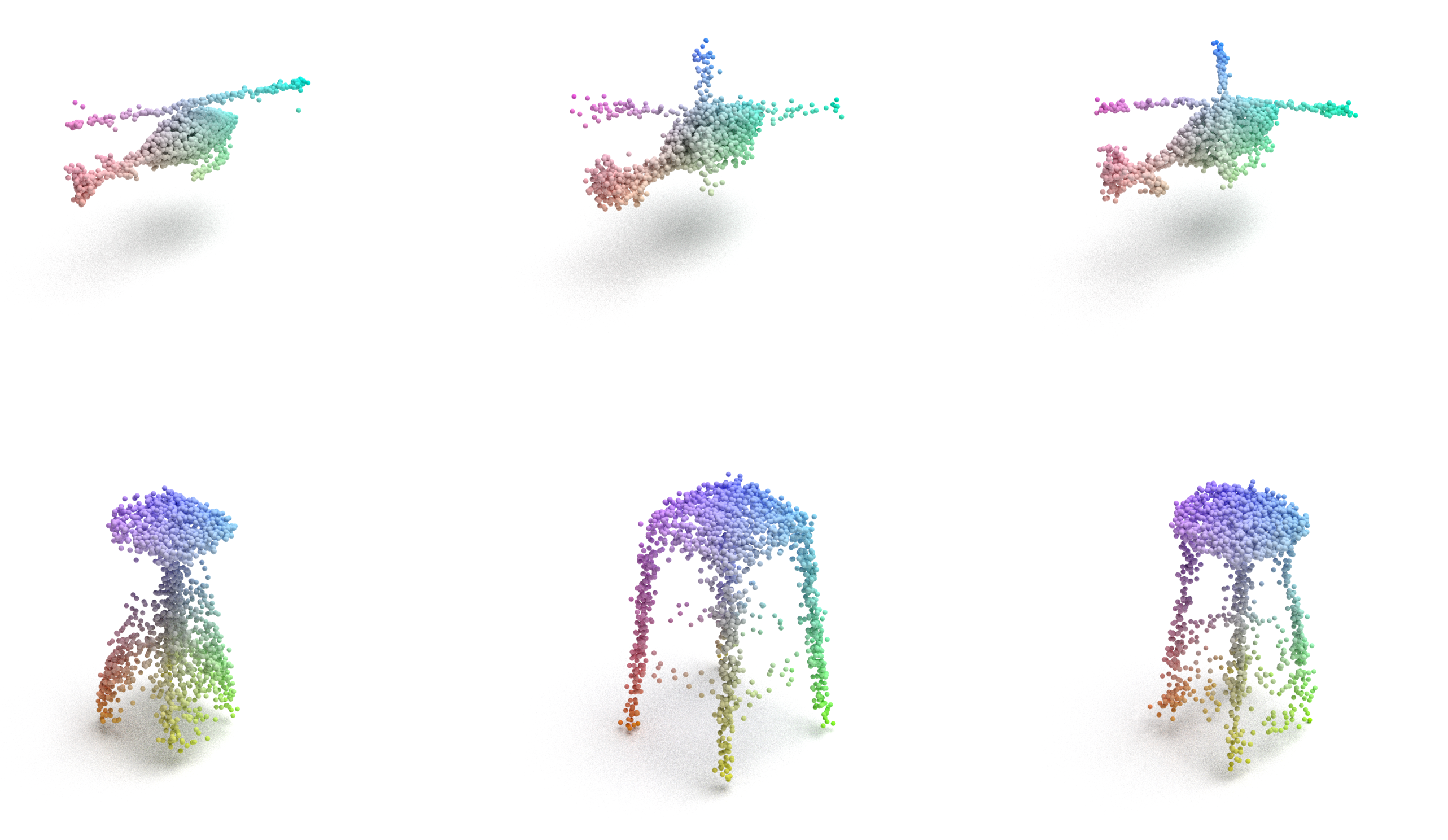
Figure 2 shows some visual comparison results. Here, we randomly pick several shape generated by RGDM given specific sub-categories. From these results, we can see that the point clouds generated by our method consists of fine details (e.g., propeller blade of helicopters) and little noise and few outlier points. The points in the shapes are also distributed uniformly, with no significant “holes”.

5.2 Controlled 3D Molecular Generations

Dataset

QM9 [30] is a dataset of 130k stable and synthetically accessible organic molecules with up to 9 heavy atoms (29 atoms including hydrogens). In this section, we train diffusion models to generate atoms’ (1) 3-dimensional coordinates; (2) types (H, C, N, O, F) and (3) integer-valued atom charges. We use the train/val/test partitions introduced in Anderson et al. 2019 (train/val/test: 100K/18K/13K samples) for evaluation.

Evaluation Metrics

Our goal here is to generate molecules targeting some desired properties while at the same time not harming general generation quality (e.g., molecules’ validity (the proportion of atoms with right valency) and stability, etc.). In such a scenario, a molecule is represented as a point cloud, in which each point denotes a single atom and has its own (atom) type. Following [35], for each pair of atoms, we use the distance between them and the atoms’ types to predict bonds (single, double, triple, or none) between atoms.

In this section, we consider optimizing two desired properties: (1) quantitative estimate of drug-likeness (QED) [2] (how likely a molecule is a potential drug candidate based on marketed drug molecules) and (2) synthetic accessibility score (SA) (the difficulty of drug synthesis), which are crucial in drug discovery domain. A good method should have a high averaged QED and SA. Note that we conduct separated experiments for these two properties, which means only one property is considered in a single experiment. We adopt widely-used open-source cheminformatics software RDKit⁴⁴ 4 https://www.rdkit.org to calculate the properties above.

Baselines

In this section, we adopt E(3) equivariant diffusion model (EDM) [14], which achieves SOTA performance in 3D conditional molecule generation, as the baseline method. EDM specifies a diffusion process that operates on both continuous coordinates and categorical atom types. Particularly, EDM adopts equivariant graph neural networks (EGNN) [36] to model molecular geometries, which are equivariant to the action of rotations, reflections and translations. For both the baseline and the proposed method, we use the neural network architecture specified in Hoogeboom et al. 2022 as the backbone. We exclude TPM [7] as a comparison method because it requires gradients from a pre-trained classifier (scoring function) to guide the controlled generation. Nevertheless, the property calculators for QED and SA are non-differentiable.

Implementation Details

For all the experiments in this section, we set the number of steps $T$ in the diffusion process to 1,000. The noise scheduling factor of step $t$ , i.e. $\beta_{t}$ , is set to the cosine noise schedule introduced in Nichol and Dhariwal 2021, Hoogeboom et al. 2022. We choose to implement the noise estimator as EGNNs with 256 hidden features and 9 layers. The rewards in RGDM come from RDKit QED and SA calculator.

5.2.1 Result Analysis

The results of controlled molecule generation are reported in Table 2. Compared with EDM, the proposed reward-guided framework RGDM generates molecules with higher QED and SA scores without hurting their general chemistry characteristics (i.e. high rate of validity and stability). Such results again demonstrate the superiority of reward-guided diffusion models over existing conditional diffusion models, such as EDM.

Table 2: Molecule stability (Mol Stable), Validity (Valid), QED and SA across 3 runs on QM9, each drawing 1,000 samples from the model.

Methods		EDM	RGDM
General Properties	Mol Stable (%)	90.7	90.5
General Properties	Valid (%)	91.2	91.4
Properties to Optimize	Avg. QED	0.461	0.542
Properties to Optimize	Avg. SA	4.41	5.87

Moreover, it is worth emphasising that the molecular point clouds are much more sparse and discontinuous than 3D shape clouds. This characteristics makes it difficult for conventional RL learners to find highly-rewarded refinements in reversed trajectories. Nevertheless, by taking advantage of the reward-aware payoff distribution, the proposed RGDM successfully overcomes such difficulty and achieves impressive performance.

6 Conclusions

This paper presents a reward-guided learning framework for diffusion models that enables flexible controlled generation. Unlike the conventional RL framework, the proposed RGDM estimates policy (model) gradients through samples from the stationary reward-aware payoff distribution rather than the policy itself. Thus, the learning objective is turned into a reward re-weighted biased noise prediction loss, which can effectively guide the reversed process towards highly-rewarded directions and simultaneously reduce variances of the estimated gradients. Experimental results on 3D shape generation and molecular generation tasks show that the proposed framework outperforms existing controlled diffusion models by a clear margin. In the future, we plan to explore more effective sampling strategies for payoff distributions to improve the model performance.

References

Anderson et al. [2019] Brandon Anderson, Truong Son Hy, and Risi Kondor. Cormorant: Covariant molecular neural networks. Advances in neural information processing systems, 32, 2019.
Bickerton et al. [2012] G Richard Bickerton, Gaia V Paolini, Jérémy Besnard, Sorel Muresan, and Andrew L Hopkins. Quantifying the chemical beauty of drugs. Nature chemistry, 4(2):90–98, 2012.
Cai et al. [2020] Ruojin Cai, Guandao Yang, Hadar Averbuch-Elor, Zekun Hao, Serge Belongie, Noah Snavely, and Bharath Hariharan. Learning gradient fields for shape generation. In European Conference on Computer Vision, pages 364–381. Springer, 2020.
Chang et al. [2015] Angel X Chang, Thomas Funkhouser, Leonidas Guibas, Pat Hanrahan, Qixing Huang, Zimo Li, Silvio Savarese, Manolis Savva, Shuran Song, Hao Su, et al. Shapenet: An information-rich 3d model repository. arXiv preprint arXiv:1512.03012, 2015.
Chen et al. [2020] Nanxin Chen, Yu Zhang, Heiga Zen, Ron J Weiss, Mohammad Norouzi, and William Chan. Wavegrad: Estimating gradients for waveform generation. arXiv preprint arXiv:2009.00713, 2020.
Choi et al. [2021] Jooyoung Choi, Sungwon Kim, Yonghyun Jeong, Youngjune Gwon, and Sungroh Yoon. Ilvr: Conditioning method for denoising diffusion probabilistic models. arXiv preprint arXiv:2108.02938, 2021.
Dhariwal and Nichol [2021] Prafulla Dhariwal and Alexander Nichol. Diffusion models beat gans on image synthesis. Advances in Neural Information Processing Systems, 34:8780–8794, 2021.
Goldfeder and Allen [2008] Corey Goldfeder and Peter Allen. Autotagging to improve text search for 3d models. In Proceedings of the 8th ACM/IEEE-CS joint conference on Digital libraries, pages 355–358, 2008.
Grathwohl et al. [2018] Will Grathwohl, Ricky TQ Chen, Jesse Bettencourt, Ilya Sutskever, and David Duvenaud. Ffjord: Free-form continuous dynamics for scalable reversible generative models. arXiv preprint arXiv:1810.01367, 2018.
Haarnoja [2018] Tuomas Haarnoja. Acquiring diverse robot skills via maximum entropy deep reinforcement learning. University of California, Berkeley, 2018.
Ho and Salimans [2022] Jonathan Ho and Tim Salimans. Classifier-free diffusion guidance. arXiv preprint arXiv:2207.12598, 2022.
Ho et al. [2020] Jonathan Ho, Ajay Jain, and Pieter Abbeel. Denoising diffusion probabilistic models. arXiv preprint arXiv:2006.11239, 2020.
Ho et al. [2022] Jonathan Ho, Chitwan Saharia, William Chan, David J Fleet, Mohammad Norouzi, and Tim Salimans. Cascaded diffusion models for high fidelity image generation. J. Mach. Learn. Res., 23:47–1, 2022.
Hoogeboom et al. [2022] Emiel Hoogeboom, Vıctor Garcia Satorras, Clément Vignac, and Max Welling. Equivariant diffusion for molecule generation in 3d. In International Conference on Machine Learning, pages 8867–8887. PMLR, 2022.
[15] https://www.yobi3d.com. Yobi3d-free 3d model search engine [online].
Kappen et al. [2012] Hilbert J Kappen, Vicenç Gómez, and Manfred Opper. Optimal control as a graphical model inference problem. Machine learning, 87(2):159–182, 2012.
Kingma et al. [2021] Diederik P Kingma, Tim Salimans, Ben Poole, and Jonathan Ho. Variational diffusion models. arXiv preprint arXiv:2107.00630, 2, 2021.
Klokov et al. [2020] Roman Klokov, Edmond Boyer, and Jakob Verbeek. Discrete point flow networks for efficient point cloud generation. In European Conference on Computer Vision, pages 694–710. Springer, 2020.
Kong et al. [2020] Zhifeng Kong, Wei Ping, Jiaji Huang, Kexin Zhao, and Bryan Catanzaro. Diffwave: A versatile diffusion model for audio synthesis. arXiv preprint arXiv:2009.09761, 2020.
Li et al. [2021] Ruihui Li, Xianzhi Li, Ka-Hei Hui, and Chi-Wing Fu. Sp-gan: Sphere-guided 3d shape generation and manipulation. ACM Transactions on Graphics (TOG), 40(4):1–12, 2021.
Liu et al. [2021] Xinhai Liu, Zhizhong Han, Yu-Shen Liu, and Matthias Zwicker. Fine-grained 3d shape classification with hierarchical part-view attention. IEEE Transactions on Image Processing, 30:1744–1758, 2021.
Luo and Hu [2021] Shitong Luo and Wei Hu. Diffusion probabilistic models for 3d point cloud generation. In Proceedings of the IEEE/CVF Conference on Computer Vision and Pattern Recognition, pages 2837–2845, 2021.
Mittal et al. [2022] Paritosh Mittal, Yen-Chi Cheng, Maneesh Singh, and Shubham Tulsiani. Autosdf: Shape priors for 3d completion, reconstruction and generation. In Proceedings of the IEEE/CVF Conference on Computer Vision and Pattern Recognition, pages 306–315, 2022.
Mnih et al. [2013] Volodymyr Mnih, Koray Kavukcuoglu, David Silver, Alex Graves, Ioannis Antonoglou, Daan Wierstra, and Martin Riedmiller. Playing atari with deep reinforcement learning. arXiv preprint arXiv:1312.5602, 2013.
Mnih et al. [2016] Volodymyr Mnih, Adria Puigdomenech Badia, Mehdi Mirza, Alex Graves, Timothy Lillicrap, Tim Harley, David Silver, and Koray Kavukcuoglu. Asynchronous methods for deep reinforcement learning. In International conference on machine learning, pages 1928–1937. PMLR, 2016.
Nichol and Dhariwal [2021] Alex Nichol and Prafulla Dhariwal. Improved denoising diffusion probabilistic models. arXiv preprint arXiv:2102.09672, 2021.
Norouzi et al. [2016] Mohammad Norouzi, Samy Bengio, Navdeep Jaitly, Mike Schuster, Yonghui Wu, Dale Schuurmans, et al. Reward augmented maximum likelihood for neural structured prediction. Advances In Neural Information Processing Systems, 29, 2016.
Peters and Schaal [2007] Jan Peters and Stefan Schaal. Reinforcement learning by reward-weighted regression for operational space control. In Proceedings of the 24th international conference on Machine learning, pages 745–750, 2007.
Qi et al. [2017] Charles R Qi, Hao Su, Kaichun Mo, and Leonidas J Guibas. Pointnet: Deep learning on point sets for 3d classification and segmentation. In Proceedings of the IEEE conference on computer vision and pattern recognition, pages 652–660, 2017.
Ramakrishnan et al. [2014] Raghunathan Ramakrishnan, Pavlo O Dral, Matthias Rupp, and O Anatole Von Lilienfeld. Quantum chemistry structures and properties of 134 kilo molecules. Scientific data, 1(1):1–7, 2014.
Ramasinghe et al. [2020] Sameera Ramasinghe, Salman Khan, Nick Barnes, and Stephen Gould. Spectral-gans for high-resolution 3d point-cloud generation. In 2020 IEEE/RSJ International Conference on Intelligent Robots and Systems (IROS), pages 8169–8176. IEEE, 2020.
Rombach et al. [2022] Robin Rombach, Andreas Blattmann, Dominik Lorenz, Patrick Esser, and Björn Ommer. High-resolution image synthesis with latent diffusion models. In Proceedings of the IEEE/CVF Conference on Computer Vision and Pattern Recognition, pages 10684–10695, 2022.
Saharia et al. [2022a] Chitwan Saharia, William Chan, Huiwen Chang, Chris Lee, Jonathan Ho, Tim Salimans, David Fleet, and Mohammad Norouzi. Palette: Image-to-image diffusion models. In ACM SIGGRAPH 2022 Conference Proceedings, pages 1–10, 2022a.
Saharia et al. [2022b] Chitwan Saharia, Jonathan Ho, William Chan, Tim Salimans, David J Fleet, and Mohammad Norouzi. Image super-resolution via iterative refinement. IEEE Transactions on Pattern Analysis and Machine Intelligence, 2022b.
Satorras et al. [2021a] Victor Garcia Satorras, Emiel Hoogeboom, Fabian Fuchs, Ingmar Posner, and Max Welling. E(n) equivariant normalizing flows. Advances in Neural Information Processing Systems, 34, 2021a.
Satorras et al. [2021b] Victor Garcia Satorras, Emiel Hoogeboom, and Max Welling. E (n) equivariant graph neural networks. arXiv preprint arXiv:2102.09844, 2021b.
Shu et al. [2019] Dong Wook Shu, Sung Woo Park, and Junseok Kwon. 3d point cloud generative adversarial network based on tree structured graph convolutions. In Proceedings of the IEEE/CVF international conference on computer vision, pages 3859–3868, 2019.
Sohl-Dickstein et al. [2015] Jascha Sohl-Dickstein, Eric A. Weiss, Niru Maheswaranathan, and Surya Ganguli. Deep unsupervised learning using nonequilibrium thermodynamics. In Francis R. Bach and David M. Blei, editors, Proceedings of the 32nd International Conference on Machine Learning, ICML, 2015.
Song and Ermon [2019] Yang Song and Stefano Ermon. Generative modeling by estimating gradients of the data distribution. CoRR, abs/1907.05600, 2019. URL http://arxiv.org/abs/1907.05600.
Song et al. [2021] Yang Song, Liyue Shen, Lei Xing, and Stefano Ermon. Solving inverse problems in medical imaging with score-based generative models. arXiv preprint arXiv:2111.08005, 2021.
Sun et al. [2020] Yongbin Sun, Yue Wang, Ziwei Liu, Joshua Siegel, and Sanjay Sarma. Pointgrow: Autoregressively learned point cloud generation with self-attention. In Proceedings of the IEEE/CVF Winter Conference on Applications of Computer Vision, pages 61–70, 2020.
Sutton et al. [1999] Richard S Sutton, David McAllester, Satinder Singh, and Yishay Mansour. Policy gradient methods for reinforcement learning with function approximation. Advances in neural information processing systems, 12, 1999.
Tang et al. [2022] Yingzhi Tang, Yue Qian, Qijian Zhang, Yiming Zeng, Junhui Hou, and Xuefei Zhe. Warpinggan: Warping multiple uniform priors for adversarial 3d point cloud generation. In Proceedings of the IEEE/CVF Conference on Computer Vision and Pattern Recognition, pages 6397–6405, 2022.
Yang et al. [2019] Guandao Yang, Xun Huang, Zekun Hao, Ming-Yu Liu, Serge Belongie, and Bharath Hariharan. Pointflow: 3d point cloud generation with continuous normalizing flows. In Proceedings of the IEEE/CVF International Conference on Computer Vision, pages 4541–4550, 2019.
Zhou et al. [2021] Linqi Zhou, Yilun Du, and Jiajun Wu. 3d shape generation and completion through point-voxel diffusion. In Proceedings of the IEEE/CVF International Conference on Computer Vision, pages 5826–5835, 2021.

Appendix A Appendix I - Detailed Derivations

A.1 Derivation from Eq. (7) to (11)

Below is the detailed derivation from Eq. (7) to (11):

\scriptsize\begin{split}&\mathcal{L}_{RL}\\ =&-\mathbb{E}_{D}\bigg\{\sum_{t=1}^{T}\big[\mathcal{H}(p_{\theta}(\mathbf{X}_{t-1}\mid\mathbf{X}_{t}))+\mathbb{E}_{p_{\theta}(\mathbf{X}_{t-1}\mid\mathbf{X}_{t})}r(\mathbf{X}_{t-1})\big]\bigg\}\\ =&-\mathbb{E}_{D}\bigg\{\sum_{t=1}^{T}\big[\int p_{\theta}(\mathbf{X}_{t-1}\mid\mathbf{X}_{t})\log p_{\theta}(\mathbf{X}_{t-1}\mid\mathbf{X}_{t})\text{d}\mathbf{X}_{t-1}+\int p_{\theta}(\mathbf{X}_{t-1}\mid\mathbf{X}_{t})r(\mathbf{X}_{t-1})\text{d}\mathbf{X}_{t-1}\big]\bigg\}\\ {\color[rgb]{0,0,0}\bm{\propto}}&-\mathbb{E}_{D}\bigg\{\sum_{t=1}^{T}\big[\int p_{\theta}(\mathbf{X}_{t-1}\mid\mathbf{X}_{t})\log p_{\theta}(\mathbf{X}_{t-1}\mid\mathbf{X}_{t})\text{d}\mathbf{X}_{t-1}-p_{\theta}(\mathbf{X}_{t-1}\mid\mathbf{X}_{t})\big(r(\mathbf{X}_{t-1})-\underbrace{\log Z+\int q(\tilde{\mathbf{X}}_{t-1}\mid\mathbf{X}_{t},\mathbf{X}_{0})\text{d}\tilde{\mathbf{X}}_{t-1}}_{Constants}\big)\text{d}\mathbf{X}_{t-1}\\ {\color[rgb]{0,0,0}\bm{\propto}}&-\mathbb{E}_{D}\bigg\{\sum_{t=1}^{T}\big[\int p_{\theta}(\mathbf{X}_{t-1}\mid\mathbf{X}_{t})\log p_{\theta}(\mathbf{X}_{t-1}\mid\mathbf{X}_{t})\text{d}\mathbf{X}_{t-1}+\int p_{\theta}(\mathbf{X}_{t-1}\mid\mathbf{X}_{t})\int p(\mathbf{X}_{t-1}\mid\tilde{\mathbf{X}}_{t-1})q(\tilde{\mathbf{X}}_{t-1}\mid\mathbf{X}_{t},\mathbf{X}_{0})\text{d}\tilde{\mathbf{X}}_{t-1}\text{d}\mathbf{X}_{t-1}\big]\bigg\}\\ =&\mathbb{E}_{D}\bigg\{\sum_{t=1}^{T}\big[\int p_{\theta}(\mathbf{X}_{t-1}\mid\mathbf{X}_{t})\bigg(\log p_{\theta}(\mathbf{X}_{t-1}\mid\mathbf{X}_{t})-\log q_{pd}(\mathbf{X}_{t-1}\mid\mathbf{X}_{t},\mathbf{X}_{0})\bigg)\text{d}\mathbf{X}_{t-1}\big]\bigg\}\\ =&\mathbb{E}_{D}\sum_{t=1}^{T}\bigg\{\big[D_{\text{KL}}(p_{\theta}(\mathbf{X}_{t-1}\mid\mathbf{X}_{t})\mid\mid q_{pd}(\mathbf{X}_{t-1}\mid\mathbf{X}_{t},\mathbf{X}_{0}))\big]\bigg\},\end{split}

(16)

where $\int q(\tilde{\mathbf{X}}_{t-1}\mid\mathbf{X}_{t},\mathbf{X}_{0})\text{d}\tilde{\mathbf{X}}_{t-1}$ and $\int p_{\theta}(\mathbf{X}_{t-1}\mid\mathbf{X}_{t})\text{d}\mathbf{X}$ are constants.

A.2 Derivation of Eq. (13)

Below is the detailed derivation of Eq. (13). Here, we introduce $\mathcal{F}(\mathbf{X}_{t-1})$ , which denotes the feasible set of $\tilde{\mathbf{X}}_{t-1}$ given $\mathbf{X}_{t-1}$ . In this paper, $\tilde{\mathbf{X}}_{t-1}$ lies within an $\ell_{2}$ ball of radius $d$ (as defined in Eq. (9)).

\scriptsize\begin{split}&\mathcal{L}_{RMLE}\\ =&\mathbb{E}\bigg\{\sum_{t=1}^{T}\int q_{pd}(\mathbf{X}_{t-1}\mid\mathbf{X}_{t},\mathbf{X}_{0})\big(\log q_{pd}(\mathbf{X}_{t-1}\mid\mathbf{X}_{t},\mathbf{X}_{0})-\log p_{\theta}(\mathbf{X}_{t-1}\mid\mathbf{X}_{t})\big)\text{d}\mathbf{X}_{t-1}\bigg\}\\ =&\mathbb{E}\bigg\{\sum_{t=1}^{T}\int\left[\int_{\mathcal{F}(\mathbf{X}_{t-1})}p(\mathbf{X}_{t-1}\mid\tilde{\mathbf{X}}_{t-1})q(\tilde{\mathbf{X}}_{t-1}\mid\mathbf{X}_{t},\mathbf{X}_{0})\text{d}\tilde{\mathbf{X}}_{t-1}\bigg(\log\int_{\mathcal{F}(\mathbf{X}_{t-1})}p(\mathbf{X}_{t-1}\mid\tilde{\mathbf{X}}_{t-1})q(\tilde{\mathbf{X}}_{t-1}\mid\mathbf{X}_{t},\mathbf{X}_{0})\text{d}\tilde{\mathbf{X}}_{t-1}\right.\\ &\left.\hskip 8.19447pt-(\frac{1}{2}\log\beta_{t}-\frac{1}{2}\log\pi-\frac{1}{2}\log 2-\frac{\|\mathbf{X}_{t-1}-\bm{\mu}_{\theta}(\mathbf{X}_{t},t)\|^{2}}{2\beta_{t}})\bigg)\right]\text{d}\mathbf{X}_{t-1}\bigg\}\hskip 16.38895pt\text{ {\color[rgb]{0,0,1}$\Longleftarrow\frac{1}{Z}\exp(r(\mathbf{X}_{t-1}))$ does not include $\tilde{\mathbf{X}}_{t-1}$.} }\\ =&\mathbb{E}\bigg\{\sum_{t=1}^{T}\int\frac{1}{Z}\exp(r(\mathbf{X}_{t-1}))\left[\int_{\mathcal{F}(\mathbf{X}_{t-1})}q(\tilde{\mathbf{X}}_{t-1}\mid\mathbf{X}_{t},\mathbf{X}_{0})\text{d}\tilde{\mathbf{X}}_{t-1}\bigg(\log\big(\frac{1}{Z}\exp(r(\mathbf{X}_{t-1}))\int_{\mathcal{F}(\mathbf{X}_{t-1})}q(\tilde{\mathbf{X}}_{t-1}\mid\mathbf{X}_{t},\mathbf{X}_{0})\text{d}\tilde{\mathbf{X}}_{t-1}\big)\right.\\ &\left.\hskip 8.19447pt-(\frac{1}{2}\log\beta_{t}-\frac{1}{2}\log\pi-\frac{1}{2}\log 2-\frac{\|\mathbf{X}_{t-1}-\bm{\mu}_{\theta}(\mathbf{X}_{t},t)\|^{2}}{2\beta_{t}})\bigg)\right]\text{d}\mathbf{X}_{t-1}\bigg\}\hskip 16.38895pt\text{ {\color[rgb]{0,0,1}$\Longleftarrow$ finite integral of Gaussian family is a constant.} }\\ =&\mathbb{E}\bigg\{\sum_{t=1}^{T}\int\frac{1}{Z}\exp(r(\mathbf{X}_{t-1}))\bigg(r(\mathbf{X}_{t-1})-\log Z+\log\int_{\mathcal{F}(\mathbf{X}_{t-1})}q(\tilde{\mathbf{X}}_{t-1}\mid\mathbf{X}_{t},\mathbf{X}_{0})\text{d}\tilde{\mathbf{X}}_{t-1}\\ &\hskip 8.19447pt-(\frac{1}{2}\log\beta_{t}-\frac{1}{2}\log\pi-\frac{1}{2}\log 2-\frac{\|\mathbf{X}_{t-1}-\bm{\mu}_{\theta}(\mathbf{X}_{t},t)\|^{2}}{2\beta_{t}})\bigg)\text{d}\mathbf{X}_{t-1}\bigg\}\\ =&\mathbb{E}\bigg\{\sum_{t=1}^{T}\int\frac{1}{Z}\exp(r(\mathbf{X}_{t-1}))\bigg(constant+\frac{\|\mathbf{X}_{t-1}-\bm{\mu}_{\theta}(\mathbf{X}_{t},t)\|^{2}}{2\beta_{t}}\bigg)\text{d}\mathbf{X}_{t-1}\bigg\}\hskip 16.38895pt\text{ {\color[rgb]{0,0,1} $\Longleftarrow$ the formulation of $r(\mathbf{X}_{t-1})$ is unknown. } }\\ \propto\;&\mathbb{E}\bigg\{\sum_{t=1}^{T}\mathbb{E}_{\mathbf{X}_{t}}\exp(r(\mathbf{X}_{t-1}))\frac{\|\mathbf{X}_{t-1}-\bm{\mu}_{\theta}(\mathbf{X}_{t},t)\|^{2}}{2\beta_{t}}\bigg\}.\end{split}

(17)