DCFace: Synthetic Face Generation with Dual Condition Diffusion Model

Minchul Kim Email: kimminc2@msu.edu Feng Liu Email: liufeng6@msu.edu Anil Jain Email: jain@msu.edu Xiaoming Liu Email: liuxm@msu.edu Michigan State University Affiliation: East Lansing, MI 48824

Abstract

Generating synthetic datasets for training face recognition models is challenging because dataset generation entails more than creating high fidelity images. It involves generating multiple images of same subjects under different factors (e.g., variations in pose, illumination, expression, aging and occlusion) which follows the real image conditional distribution. Previous works have studied the generation of synthetic datasets using GAN or 3D models. In this work, we approach the problem from the aspect of combining subject appearance (ID) and external factor (style) conditions. These two conditions provide a direct way to control the inter-class and intra-class variations. To this end, we propose a Dual Condition Face Generator (DCFace) based on a diffusion model. Our novel Patch-wise style extractor and Time-step dependent ID loss enables DCFace to consistently produce face images of the same subject under different styles with precise control. Face recognition models trained on synthetic images from the proposed DCFace provide higher verification accuracies compared to previous works by $6.11\%$ on average in $4$ out of $5$ test datasets, LFW, CFP-FP, CPLFW, AgeDB and CALFW. Code Link

1 Introduction

What does it take to create a good training dataset for visual recognition? An ideal training dataset for recognition tasks would have 1) large inter-class variation, 2) large intra-class variation and 3) small label noise. In the context of face recognition (FR), it means, the dataset has a large number of unique subjects, large intra-subject variations, and reliable subject labels. For instance, large-scale face datasets such as WebFace4M zhu2021webface260m contain over $1$ M subjects and large number of images/subject. Both the number of subjects and the number of images per subject are important for training FR models deng2019arcface; kim2022adaface. Also, datasets amassed by crawling the web are not free from label noise zhu2021webface260m; cao2018vggface2.

Refer to caption — Figure 1: Illustration of three factors that characterize a labeled face dataset. It contains large subject variation, style variation and label consistency. Synthetic face datasets should be created with all three factors in mind. Face images in this figure are samples generated by our proposed method which combines arbitrary ID condition with style condition while preserving subject identity.

In various domains, synthetic datasets are traditionally used to help generalize deep models when only limited real datasets could be collected engelsma2022printsgan; tremblay2018training; zunair2021synthesis; hu2021sail or when bias exists in the real dataset kupas2021solving; van2021decaf. Lately, more attention has been drawn to training with only synthetic datasets in the face domain, as synthetic data can avoid leaking the privacy of real individuals. This is important as real face datasets have been under scrutiny for their lack of informed consent, as web-crawling is the primary means of large-scale data collection msceleb; zhu2021webface260m; casia. Also, synthetic training datasets can remedy some long-standing issues in real datasets, e.g. the long tail distribution, demographic bias, etc.

When it comes to generating synthetic training datasets, the following questions should be raised. (i) How many novel subjects can be synthesized (ii) How well can we mimic the distribution of real images in the target domain and (iii) How well can we consistently generate multiple images of the same subjects? We start with the hypothesis that face dataset generation can be formulated as a problem that maximizes these criteria together.

Previous efforts in generating synthetic face datasets touch on one of the three aspects but do not consider all of them together qiu2021synface; bae2022digiface. SynFace qiu2021synface generates high-fidelity face images based on DiscoFaceGAN deng2020disentangled, coming close to real images in terms of FID metric fid. However, we were surprised to find that the actual number of unique subjects that can be generated by DiscoFaceGAN is less than $500$ , a finding that will be discussed in Sec. 3.1. The recent state of the art (SoTA), DigiFace bae2022digiface, can generate $1$ M large-scale synthetic face images with many unique subjects based on $3$ D parametric model rendering. However, it falls short in matching the quality and style of real face images.

We propose a new data generation scheme that addresses all three criteria, i.e. the large number of novel subjects (uniqueness), real dataset style matching (diversity) and label consistency (consistency). In Fig. 1, we illustrate the high-level idea by showcasing some of our generated face samples. The key motivation of our paper is that the synthetic dataset generator needs to control the number of unique subjects, match the training dataset’s style distribution and be consistent in the subject label.

In light of this, we formulate the face image generation as a dual condition inverse problem, retrieving the unknown image $\mathbf{Y}$ from the observable Identity condition $\mathbf{X}_{id}$ and Style condition $\mathbf{X}_{sty}$ . Specifically, $\mathbf{X}_{id}$ specifies how a person looks and $\mathbf{X}_{sty}$ specifies how $\mathbf{X}_{id}$ should be portrayed in an image. $\mathbf{X}_{sty}$ contains identity-independent information such as pose, expression, and image quality.

Our choice of dual conditions (identity and style) is important in how we generate a synthetic dataset as ID and style conditions are controllable factors that govern the dataset’s characteristics. To achieve this, we propose a two-stage generation paradigm. First, we generate a high-quality face image $\mathbf{X}_{id}$ using a face image generator and sample a style image $\mathbf{X}_{sty}$ from a style bank. Secondly, we mix these two conditions using a dual condition generator which predicts an image that has the ID of $\mathbf{X}_{id}$ and a style of $\mathbf{X}_{sty}$ . An illustration is given in Fig. 2.

Training the mixing generator in stage 2 is not trivial as it would require a triplet of ( $\mathbf{X}^{A}_{id},\mathbf{X}^{B}_{sty}$ , $\mathbf{X}^{A}_{sty}$ ) where $\mathbf{X}^{A}_{sty}$ is a hypothetical combination of the ID of subject $A$ and the style of subject $B$ . To solve this problem, we propose a new dual condition generator that can learn from ( $\mathbf{X}^{A}_{id},\mathbf{X}^{A}_{sty}$ ), a tuple of same subject images that can always be obtained in a labeled dataset. The novelty lies in our style condition extractor and ID loss which prevents the training from falling into a degenerate solution. We modify the diffusion model sohl2015deep; ho2020denoising to take in dual conditions and apply an auxiliary time-dependent ID loss that can control the balance between sample diversity and label consistency.

We show that our Dual Condition Face Dataset Generator (DCFace) is capable of surpassing the previous methods in terms of FR performance, establishing a new benchmark in face recognition with synthetic face datasets. We also show the roles dataset subject uniqueness, diversity and consistency play in face recognition performance.

The followings are the contributions of the paper.

•

We propose a two-stage face dataset generator that controls subject uniqueness, diversity and consistency.
•

For this, we propose a dual condition generator that mixes the two independent conditions $\mathbf{X}_{id}$ and $\mathbf{X}_{sty}$ .
•

We propose uniqueness, consistency and diversity metrics that quantify the respective properties of a given dataset, useful measures that allow one to compare datasets apart from the recognition performance.
•

We achieve SoTA in FR with $0.5$ M image synthetic training dataset by surpassing the previous methods by $6.11\%$ on average in $5$ popular test datasets.

2 Related Works

Face Recognition. Face Recognition (FR) is the task of matching query imagery to an enrolled identity database. SoTA FR models are trained on large-scale web-crawled datasets zhu2021webface260m; msceleb; deng2019arcface with margin-based softmax losses wang2018cosface; deng2019arcface; liu2017sphereface; huang2020curricularface; kim2022adaface. The FR performance is measured on various benchmark datasets such as LFW lfw, CFP-FP cfpfp, CPLFW cplfw, AgeDB agedb and CALFWcalfw. These datasets are designed to measure factors such as pose changes and age variations. Performance on these datasets for models trained on large-scale datasets such as WebFace260M is well above $97\%$ kim2022adaface in verification accuracy.

Synthetic Face Generation. Recent advances in generative models allow high fidelity synthetic face image generations karras2019style; choi2018stargan; karras2017progressive; karras2020analyzing; brock2018large; ho2020denoising; song2020denoising. GANs have been widely used to manipulate, animate or enhance face images hu2018disentangling; deng2020disentangled; xiao2018elegant; pumarola2018ganimation; sun2019single; choi2018stargan; lin2018conditional; disentangled-representation-learning-gan-for-pose-invariant-face-recognition. They typically learn disentangled representations in GAN latent space that control desired face properties. On the contrary, some works leverage the 3D face prior from 3D datasets (e.g., $3$ DMM blanz1999morphable) for controllable synthesis shen2018facefeat; kim2018deep; deng2018uv; gecer2018semi; geng20193d; piao2019semi; nguyen2019hologan; most-gan-3d-morphable-stylegan-for-disentangled-face-image-manipulation. These methods have advantages in the fine-grained control over face generation and 3D consistency yet lack in style or domain variation.

Recent advances in the latent variable models such as diffusion or score-based models have shown great success in high-quality image generation with a more stable and simple objective of MSE loss ho2020denoising; nichol2021improved; sohl2015deep; song2019generative; song2020improved; song2021maximum; song2020denoising. Diffusion models have advanced the conditional image generation in tasks such as text-conditional image generation, inpainting, etc piti; dalle2; blattmann2022retrieval; rombach2022high. We adopt the diffusion model as a backbone and explore how the two image characteristics, namely ID and style images, can control complementary information, the subject appearance and the style of an image.

Face Recognition with Synthetic Dataset. Synthetic training datasets offer an advantage over real datasets with regards to ethical issues and class imbalance problems as large-scale face datasets have been criticized for lacking informed consent and reflecting racial biases zhu2021webface260m; deng2019arcface; yi2014learning; bae2022digiface. Despite the benefit, use of synthetic datasets as the sole training data is not widely adopted due to the resulting low recognition performance. In various domains such as face recognition qiu2021synface; bae2022digiface; controllable-and-guided-face-synthesis-for-unconstrained-face-recognition, fingerprint recognition engelsma2022printsgan; wyzykowski2022synthetic, and anti-spoofing 9779478; noise-modeling-synthesis-and-classification-for-generic-object-anti-spoofing, synthetic datasets have been shown to improve recognition when combined with real images.

In the face domain, SynFace qiu2021synface studied the efficacy of using DiscoFaceGAN deng2020disentangled for synthetic face generation. Recently, DigiFace-1M bae2022digiface studied the efficacy of 3D model based face rendering in combination with image augmentations to create a synthetic dataset. We propose a face dataset generation method that can generate both a large number of subjects and diverse styles that are close to the real dataset.

3 Proposed Approach

We propose Dual Condition Face Dataset Generator (DCFace), a two-stage dataset generator (see Fig. 2). Stage $1$ is the Condition Sampling Stage, generating a high-quality ID image ( $\mathbf{X}_{id}$ ) of a novel subject and selects one arbitrary style image ( $\mathbf{X}_{sty}$ ) from the bank of real training data. Stage $2$ is the Mixing Stage which combines the two images using the Dual Condition Generator.

For trainable models in each stage, Stage $1$ requires training an ID image generator $G_{id}$ . For the style bank, we can conveniently use any real face dataset that we wish generated samples to follow. Stage $2$ requires training a dual condition mixer $G_{mix}$ . Both $G_{id}$ and $G_{mix}$ are based on diffusion models ho2020denoising. We describe each component and the associated training procedure in the following subsections.

Figure 3: Comparison of the number of unique subjects generated by DiscoFaceGAN deng2020disentangled and unconditional DDPM ho2020denoising. Uniqueness is the number of unique subjects measured by a face recognition model. By varying the threshold which determines a match between two subjects, we plot the number of unique subjects as defined in Eq. 11. Unconditional DDPM and DiscoFaceGAN are trained on FFHQ karras2019style and each generates

10,000

samples. The ability to generate novel subjects is larger for DDPM. Refer to Supp.E for additional details on the threshold.

3.1 Preliminary

Diffusion models sohl2015deep; ho2020denoising are a class of denoising generative models that are trained to predict an image from random noise through a gradual denoising process. One notable difference from the class of GAN-based generators goodfellow2020generative is in the objective function and the sampling procedure. The forward process as expressed in Eq. 1 corrupts the input $\bm{X}$ using variance controlled Gaussian noise over $t$ time-steps,

q\left(\bm{\bm{X}}_{t}|\bm{\bm{X}}_{t-1}\right)=\mathcal{N}\left(\bm{\bm{X}}_{t};\sqrt{1-\beta_{t}}\bm{\bm{X}}_{t-1},\beta_{t}\bm{I}\right),

(1)

and the denoising is done by training a model $\bm{\epsilon}_{\theta}(\bm{X}_{t},t)$ to predict the initial noise $\bm{\epsilon}$ with an $L_{2}$ objective,

\mathcal{L}=\mathbb{E}_{t,\bm{X}_{0},\bm{\epsilon}}\Big[\big\|\bm{\epsilon}_{\theta}(\underbrace{\sqrt{\alpha_{t}}\bm{X}_{0}+\sqrt{1-\alpha_{t}}\bm{\epsilon}}_{\bm{X}_{t}},t)-\bm{\epsilon}\big\|_{2}^{2}\Big].

(2)

$\beta_{t}$ and $\alpha_{t}$ are pre-set variance scheduling scalars. The denoising diffusion model (DDPM) has shown success in producing diverse samples in text-conditioned image generation dalle2. We find that in unconditional face generation, DDPM is also capable of generating many unique subjects. For instance, Fig. 3 compares DiscoFaceGAN deng2020disentangled with DDPM ho2020denoising in their capacity to generate different subjects for every sample. It shows that DDPM ho2020denoising is a good model choice for $G_{id}$ and $G_{mix}$ as it can generate many unique subjects. For $G_{id}$ , we adopt the unconditional DDPM trained on FFHQ karras2019style, having observed that it is capable of generating a large number of unique subject images.

3.2 Dual Condition Generator $G_{mix}$

The two-stage data generation requires Dual Condition Generator $G_{mix}$ which is a conditional DDPM. Two conditions $\bm{X}_{id}$ and $\bm{X}_{sty}$ are injected into the denoiser $\bm{\epsilon}_{\theta}(\bm{X}_{t},t,E_{id}(\bm{X}_{id}),E_{sty}(\bm{X}_{sty}))$ using trainable feature extractors $E_{id}$ and $E_{sty}$ and cross-attentions. $G_{mix}$ is responsible for the operation $\bm{X}_{id}^{A}+\bm{X}_{sty}^{B}\!\rightarrow\!\bm{X}_{sty}^{A}$ , a mixing of an image of a novel subject $A$ and an arbitrary style image of different subject $B$ .

Naive training would require the reference image $\bm{X}_{sty}^{A}$ , an image of subject $A$ in the style of $\bm{X}_{sty}^{B}$ . This reference is absent in the labeled training dataset. As such, we modify the operation to $\bm{X}_{id}^{A}+\bm{X}_{sty}^{A}\!\rightarrow\!\bm{X}_{sty}^{A}$ , using two different images from the same subject as illustrated in Fig. 4(a). But this formulation is prone to a trivial solution of ignoring $\bm{X}_{id}^{A}$ , making the ID condition unused during test time. To mitigate this issue, we propose the following two elements.

Patch-wise Style Extractor $E_{sty}$ . The motivation of Style Extractor is to map an image $\bm{X}_{sty}$ to a feature that contains little ID information, forcing $G_{mix}$ to rely on $\bm{X}_{id}$ for ID information. In prior works such as StyleGAN, $1^{st}$ and $2^{nd}$ order statistics of a feature are shown to resemble the image style karras2019style; caface; lee2019srm. Yet, resulting statistics are reduced in spatial dimensions and consequently without spatially local informations such as pose.

We propose a module that can extract style information without losing spatial information. Specifically, consider a pretrained and fixed face recognition model $F_{s}$ and its intermediate feature $F_{s}(\mathbf{X}_{sty})=\mathbf{I}_{sty}\!\in\!\mathbb{R}^{C\!\times\!H\!\times\!W}$ . We divide the feature into a $k\times\!k$ grid. For each element in the grid $\mathbf{I}_{sty}^{k_{i}}\!\in\!\mathbb{R}^{C\!\times\!\frac{H}{k}\!\times\!\frac{W}{k}}$ , we perform non-linear mapping on the mean and variance of $\mathbf{I}_{sty}^{k_{i}}$ . Specifically,

	$\displaystyle\mathbf{\hat{I}}^{k_{i}}=\text{BN}(\text{Conv}(\text{ReLU}(\text{Dropout}(\mathbf{I}_{sty}^{k_{i}})))),$		(3)
	$\displaystyle\bm{\mu}_{\text{sty}}^{k_{i}}=\text{SpatialMean}(\mathbf{\hat{I}}^{k_{i}}),\quad\bm{\sigma}_{\text{sty}}^{k_{i}}=\text{SpatialStd}(\mathbf{\hat{I}}^{k_{i}}),$		(4)
	$\displaystyle\bm{s}^{k_{i}}=\text{LN}\left((\bm{W}_{1}\odot\bm{\mu}_{\text{sty}}^{k_{i}}+\bm{W}_{2}\odot\bm{\sigma}_{\text{sty}}^{k_{i}})+\bm{P}_{emb}\right),$		(5)
	$\displaystyle E_{sty}(\bm{X}_{sty}):=\bm{s}=[\bm{s}^{1},\bm{s}^{2},\bm{s}^{k_{i}}...,\bm{s}^{k\!\times\!k},\bm{s}^{\prime}],$		(6)

where $\bm{s}^{\prime}$ corresponds to $\mathbf{I}_{sty}^{k_{i}}$ being a global feature, where $k\!=\!1$ . The final output $\bm{s}$ is a concatenation of all style vectors for each patch. Each $\bm{s}^{k_{i}}$ is a mean and variance of local information which is constrained from containing full pixel-level details with the ID information. And $\bm{P}_{emb}$ is a learned position embedding to let the model differentiate different patch locations. BN and LN are BatchNorm ioffe2015batch and LayerNorm ba2016layer. $F_{s}$ is a shallow CNN taken from the early layers of a pretrained FR model. It is fixed and not updated to prevent it from optimizing $\mathbf{I}_{sty}$ , serving only to create style information. By varying the grid size $k\!\times\!k$ , we can represent style at different spatial locations. An illustration of $E_{sty}$ can be found in Fig. 4(b).

Figure 5: Illustration of conditional distributions in 2D space. Colored regions represent the true data distribution with individual colors representing different labels. Colored triangles represent generated samples with corresponding labels. For each scenario except (a), the generated distribution does not follow the true distribution. Consistency, diversity and uniqueness analysis can quantify the shortcomings.

Time-step Dependent ID Loss. To train Dual Condition Generator $G_{mix}$ , the original DDPM objective of $L_{2}$ loss, Eq. 2 is not sufficient to guarantee the consistency in subject identity between the ID condition $\bm{X}_{id}$ and the prediction, $\hat{\bm{X}}_{0}$ . To ensure the ID consistency, one could devise a loss function to maximize the similarity between $\bm{X}_{id}$ and the predicted denoised image $\hat{\bm{X}}_{0}$ , in the ID feature space using a pretrained FR model, $F$ . Specifically, following the Eq.15 of DDPM ho2020denoising, one-step prediction of the original image is

\displaystyle\hat{\bm{X}}_{0}=(\bm{X}_{t}-\sqrt{1-\bar{\alpha}_{t}}\bm{\epsilon}_{\theta}(\bm{X}_{t},t,\bm{X}_{id},\bm{X}_{sty}))/\sqrt{\bar{\alpha}_{t}}.

(7)

A simple ID loss to increase cosine similarity (CS) is

L_{\text{naive1}}=-\text{CS}\left(F(\bm{X}_{id}),F(\hat{\bm{X}}_{0}))\right).

(8)

However, this loss is in conflict with MSE loss and is empirically observed to reduce the predicted image quality. This is because the FR model, $F$ is not invariant to image style; some style of $\bm{X}_{id}$ has to match in order to completely reduce $L_{\text{naive1}}$ . In contrast, one could also use

L_{\text{naive2}}=-\text{CS}\left(F(\bm{X}_{sty}),F(\hat{\bm{X}}_{0}))\right),

(9)

as during training the label of $\bm{X}_{sty}$ and $\bm{X}_{id}$ are the same. However, $L_{\text{naive2}}$ causes the model to depend on $\bm{X}_{sty}$ for ID information. Thus, during evaluation, when $\bm{X}_{sty}$ and $\bm{X}_{id}$ are different subjects, the label consistency in the generated dataset is compromised. We show this in Tab. 2.

Instead, we propose to interpolate between $F(\bm{X}_{id})$ and $F(\bm{X}_{sty})$ across diffusion time-steps. Specifically,

\begin{split}L_{\text{ID}}=&-\gamma_{t}\text{CS}\left(F(\bm{X}_{id}),F(\hat{\bm{X}}_{0}))\right)\\ &-(1-\gamma_{t})\text{CS}\left(F(\bm{X}_{sty}),F(\hat{\bm{X}}_{0}))\right),\vskip-8.53581pt\end{split}

(10)

where $\gamma_{t}\!=\!\frac{t}{T}$ is a time-dependent weight that linearly changes from $0$ to $1$ . When $t\!=\!T$ , $\bm{\epsilon}_{\theta}$ is predicting $\bm{X}_{t-1}$ from random noise, and we let the model fully exploit the ID information of $\bm{X}_{id}$ . Gradually as $t$ increases, we let the model’s prediction walk into the direction of $\bm{X}_{sty}$ . Note that during training, the actual label of $\bm{X}_{sty}$ and $\bm{X}_{id}$ are the same. So the interpolation in the loss forces the prediction to be the same in identity but gradually shifting in style toward $\bm{X}_{sty}$ . This loss allows $\bm{\epsilon}_{\theta}(\bm{X}_{t},t,\bm{X}_{id},\bm{X}_{sty}))$ to play different roles depending on $t$ . For $t\approx T$ , $\bm{\epsilon}_{\theta}$ will exploit $\bm{X}_{id}$ to infer front-view ID rich image. And as $t\rightarrow 0$ , it will change the image’s style to match the style of $\bm{X}_{sty}$ . The final loss is $L_{MSE}+\lambda L_{ID}$ with $\lambda$ as a scaling parameter.

$\bm{E}_{id}$ and Conditioning Mechanism. Following the success text-conditional image generation and inpainting using DDPM dalle2; piti; diffae, we adopt a similar architecture for inserting conditions into the model. We concatenate $E_{id}(\bm{X}_{id})$ and $E_{sty}(\bm{X}_{sty})$ and put in $\bm{\epsilon}_{\theta}$ using cross-attention and adaptive group normalization layers (AdaGN) diffae. $E_{id}$ is a CNN, with the same architecture as a small FR model (e.g. ResNet50). And $E_{id}$ is trained end-to-end with $\bm{\epsilon}_{\theta}$ to extract useful ID feature for $\bm{\epsilon}_{\theta}$ . More training details can be found in Supp.

3.3 Condition Sampling Strategy

ID Image Sampling. For sampling ID images, we generate $200,000$ facial images from $G_{ID}$ , from which we remove faces that are wearing sunglasses or too similar to the subjects in CASIA-WebFace with the Cosine Similarity threshold of $0.3$ using $F_{eval}$ . We are left with $105,446$ images. Then we narrow them down to $62,570$ images that are unique according to uniqueness, Eq. 11 using $F_{eval}$ and $r=0.3$ . Then we explore two different options, 1) random sampling and 2) gender/ethnicity balanced sampling as $G_{id}$ has a skewed distribution towards White subjects as shown in Tab. 1. We use faceparsing to classify the ethnicity and use glasses; glassesgit to detect sunglasses. We denote the sampling option 1 as random and 2 as balance.

Style Image Sampling. For style sampling, for each $\mathbf{X}_{id}$ , we randomly sample $\mathbf{X}_{sty}$ from the style bank. We denote this option as random. We also explore the option of sampling $\mathbf{X}_{sty}$ from the pool of images whose gender/ethnicity matches that of $\mathbf{X}_{id}$ . We denote this option as match.

	White	Asian	Others	Black	Indian
CASIA-WebFace	$0.634$	$0.144$	$0.074$	$0.074$	$0.072$
DDPM $G_{id}$	$0.660$	$0.209$	$0.034$	$0.046$	$0.048$
Balanced Ethnicity	$0.200$	$0.200$	$0.200$	$0.200$	$0.200$

Table 1: Ethnicity Distribution of CASIA-WebFace. Ethnicity prediction is made using faceparsing. DDPM

G_{id}

is trained on FFHQ karras2019style.

4 Dataset Evaluation

In evaluating the synthesized dataset, one often adopts 1) FID fid for evaluating the distribution similarity to the real images and 2) subsequent recognition performance. In this section, we propose three class-dependent metrics that aid us in understanding the property of generated labeled datasets. We let $F_{eval}$ be an recognition model used for evaluating synthesized face datasets. Note that this is different from $F$ in ID loss. $F$ is a model for training loss and $F_{eval}$ is for evaluating metrics. The more generalizable $F_{eval}$ is, the more accurate the metrics become in capturing the identity and diversity of the synthesized dataset.

Let $y_{c}$ be a class label, and $f_{i}=F_{eval}(\bm{X}_{i})$ . Let $d(f_{i},f_{j})$ be the distance between two images in $F_{eval}$ feature space.

Uniqueness. Consider the following non-overlapping $r$ -ball in $F_{eval}$ space,

U\!=\!\{f_{i}:d(f_{i},f_{j})>r,\;j<i,\;i,j\in\{1,..,N\}\},

(11)

where $d(f_{i},f_{j})$ is the cosine distance. Then $|U|$ is the count of unique subjects determined by the threshold $r$ in an unlabeled dataset. Note that the set $U$ is equivalent to sequentially adding a $r$ -ball into $F_{eval}$ -space until you cannot add more without collision. $|U|$ is subject to both $r$ and $F_{eval}$ . In FR, $r$ is a threshold in the FR model that is set to determine match or non-match.

For a labeled synthetic dataset, one generates multiple feature sets $\{f_{i}^{c}\}$ for the same label. To count the number of unique subjects, we calculate the number of unique centers, $f^{c}=\frac{1}{N_{c}}\sum_{i}^{N_{c}}f_{i}^{c}$ for $c\in\{1,...,C\}$ , where $C$ is the number of subjects and $N_{c}$ is the number of images per subject. Then we define the number of unique subjects in a labeled dataset with $|U_{c}|$ where $U_{c}$ is

U_{c}\!=\!\{f_{c}\!:\!d(f^{c_{n}},f^{c_{m}})\!>\!r,m\!<\!n,n,m\!\in\!\{1,..,C\}\},

(12)

For the metric, we use $U_{class}=|U_{c}|/C$ , the ratio between the number of unique subjects and the number of labels.

Intra-class Consistency. It measures how consistent the generated samples are in adhering to the label condition, as

C_{intra}=\frac{1}{C}\sum_{c=1}^{C}\frac{1}{N_{c}}\sum_{i=1}^{N_{c}}d(f_{i}^{c},f^{c})<r,

(13)

which is the ratio of individual features $f_{i}^{c}$ being close to the class center $f^{c}$ . For a given threshold $r$ , higher values of $C_{intra}$ mean the samples are more likely to be the same subject under the same label.

Intra-class Diversity. It measures how diverse the generated samples are under the same label condition. Note that the diversity is in the style of an image, not in the subject’s identity. We define the style space as a vector space defined by Inception Network salimans2016improved features pretrained on ImageNet deng2009imagenet following the convention of kynkaanniemi2019improved, denoting the real and generated image inception vectors as $\{s_{i}^{c}\}$ , $\{\hat{s}_{j}^{c}\}$ .

For intra-class diversity, we measure how many real images fall into the style space manifold defined by the generated images under the same label condition. We compute this by extending the Improved Recall Metric kynkaanniemi2019improved, from comparing the unconditional distributions of real and fake images to comparing the label-conditional distributions. Specifically, for a set of real and generated feature vectors $\{s_{i}^{c}\}$ , $\{\hat{s}_{j}^{c}\}$ under the same label condition $y_{c}$ , we define $k$ -nearest feature distance $r_{k}$ as $r_{k}=d\bigl(\hat{s}_{j}^{c}-\text{NN}_{k}\left(\hat{s}_{j}^{c},\{\hat{s}_{j}^{c}\}\right)\bigr)$ , where $\text{NN}_{k}$ returns the $k$ -nearest feature vector in $\{\hat{s}_{j}^{c}\}$ and

\small\mathbf{I}(s_{i}^{c},\{\hat{s}_{j}^{c}\})\!=\!\begin{cases}1,\exists\hat{s}_{j}^{c}\in\{\hat{s}_{j}^{c}\}\text{ s.t. }d\left(s_{i}^{c}-\hat{s}_{j}^{c}\right)\leq r_{k}\\ 0,\text{ otherwise}.\end{cases}

(14)

$d(\cdot)$ is an Euclidean distance. Then diversity is defined by

\text{D}_{intra}=\frac{1}{C}\frac{1}{N}\sum_{c=1}^{C}\sum_{i=1}^{N_{c}}\mathbf{I}(s_{i}^{c},\{\hat{s}_{j}^{c}\}),

(15)

which is the fraction of real image styles manifold covered by the generated image style manifold as defined by $k$ -nearest neighbor ball. If the style variation is small, then $r_{k}$ becomes small, reducing the chance of $d\left(s_{i}^{c}-\hat{s}_{j}^{c}\right)\leq r_{k}$ . We compute the recall per class to capture style variation conditional on the subject label.

In Fig. 5, we illustrate different scenarios of conditional generation and how these metrics can capture the shortcomings in each scenario. In Sec. 5 and Fig. 6, we measure the metrics on our generated datasets and compare with previous synthetic datasets qiu2021synface; bae2022digiface. We find that FR performance is at best when consistency and diversity are balanced. Also, we find SynFace and DigiFace have high $C_{intra}$ and low $D_{intra}$ compared to our method in Fig. 5.

Figure 6: A plot of FR performance on

5

synthetic datasets with respect to Consistency and Diversity metrics. Color intensity and circle size denotes the FR accuracy.

5 Experiments

For $G_{id}$ which generates ID images, we adopt the publicly released unconditional DDPM ho2020denoising trained on FFHQ karras2019style. For $G_{mix}$ , we train it on CASIA-WebFace casia after initializing weights from $G_{id}$ . Although using all of CASIA-WebFace is a valid setting, we split it into a $95$ - $5$ split between train and validation sets. The validation set is used as a real dataset in measuring the uniqueness, consistency and diversity metrics. $G_{mix}$ is trained for $10$ epochs with a batch-size of $256$ using AdamW Optimizer kingma2014adam; loshchilov2017decoupled with the learning rate of $0.001$ . Training takes $8$ hours using two A100 GPUs. Once $G_{mix}$ is trained, we use $G_{id}$ , $G_{mix}$ and a style bank to generate a synthetic labeled dataset. The style bank is the CASIA-WebFace training set. For sampling, we use DDIM song2020denoising with $200$ intervals. Generating $500$ K samples takes about $20$ hours using one A100 GPU.

To train FR models, for a fair comparison, we adopt the training scheme of bae2022digiface; qiu2021synface using IR-SE-50 deng2019arcface as a backbone and AdaFace kim2022adaface as a loss function. We evaluate the trained FR models on five datasets, LFW lfw, CFP-FP cfpfp, CPLFW cplfw, AgeDB agedb and CALFWcalfw. CFP-FP and CPLFW are designed to measure the FR in the large pose variation and AgeDB and CALFW are for the large age variation. To measure the consistency, diversity and uniqueness during evaluation, we adopt $F_{eval}$ as IR101 deng2019arcface model trained on WebFace4M zhu2021webface260m with AdaFace kim2022adaface loss.

Grid Size	Loss	Loss Model	$U_{class}$	$C_{intra}$	$D_{intra}$	FR Perf.
SynFace	-	-	$0.080$	$0.9966$	$0.131$	$74.75$
DigiFace	-	-	$0.178$	$0.9973$	$0.297$	$83.45$
$1\!\times\!1$	$L_{ID}$	$F$	$\bm{0.978}$	$\bm{0.9987}$	$0.4418$	$79.28$
$3\!\times\!3$			$0.956$	$0.9809$	$0.7030$	$85.79$
$\bm{5\!\times\!5}$			$0.924$	$0.9035$	$0.7734$	$\bm{89.04}$
$7\!\times\!7$			$0.690$	$0.5937$	$\bm{0.7950}$	$50.00$
$5\!\times\!5$	$L_{naive1}$	$F$	$\bm{0.988}$	$\bm{0.9996}$	$0.6546$	$84.75$
	$L_{naive2}$		$0.866$	$0.8046$	$0.7835$	$50.00$
	$\bm{L_{ID}}$		$0.924$	$0.9035$	$\bm{0.7734}$	$\bm{89.04}$
$5\!\times\!5$	$L_{ID}$	$\bm{F}$	$0.924$	$0.9035$	$0.7734$	$89.04$
$5\!\times\!5$	$L_{ID}$	$F_{bigger}$	$\bm{0.954}$	$\bm{0.9197}$	$0.7715$	$\bm{89.89}$

Table 2: Model Ablation. For FR performance, we generate a synthetic dataset of

10K

subjects with

50

images per subject using (random, random) ID and style sampling strategy. Blue color indicates the adopted setting for subsequent experiments.

5.1 Model Ablation

To show the efficacy of our proposed modules, we ablate on 1) the grid size in Style extractor $E_{sty}$ , 2) Time-step dependent ID loss and 3) the ID loss backbone $F$ ’s. The number of samples we generate for the ablation are $10K$ subjects with $50$ images per subject, similar to CASIA-WebFace image counts. We report the FR performance with the synthetic data by averaging the $5$ validation set verification accuracies. To measure $U_{class}$ , $C_{intra}$ and $D_{intra}$ , we use $500$ subjects with $20$ real images from the held-out validation set of CASIA-WebFace and generate an equivalent number of images from each method.

Grid Size. We choose $4$ grid sizes ranging from $1\!\times\!1$ to $7\!\times\!7$ . Note that $1\!\times\!1$ corresponds to the style vector of a whole image. We expect to see higher spatial control in $\bm{X}_{sty}$ as the grid size increases. In Tab. 2, we report the three metrics $U_{class}$ , $C_{intra}$ and $D_{intra}$ . As the grid size increases, $E_{sty}$ features contain more fine-grained information, possibly related to ID, lowering the consistency. However, the diversity increases, making the conditional distribution similar to the real dataset. The subsequent FR performance using the model is the best in the setting $5\!\times\!5$ , which is a good compromise between consistency and diversity. In Fig. 7, we show the effect of the grid size with examples.

ID Loss. For ID loss, we compare $L_{\text{ID}}$ with $L_{\text{naive1}}$ and $L_{\text{naive2}}$ in Tab. 2. Using $L_{\text{naive1}}$ or $L_{\text{naive2}}$ both suffer from lower FR performance, but for different reasons. $L_{\text{naive1}}$ has low diversity because it is optimized to be similar to $\bm{X}_{id}$ of front-view high quality face images. $L_{\text{naive2}}$ has low consistency because of the lack of dependence on $\bm{X}{id}$ , making the resulting dataset with random labels. FR performance of $0.5$ means the model diverged and is returning random predictions. $L_{\text{ID}}$ , a linear interpolation of the $L_{\text{naive1}}$ and $L_{\text{naive2}}$ across time-steps results in the best performance.

ID Loss Backbone $\bm{F}$ . ID Loss requires a pretrained FR model, $F$ . For all of our experiments, we use $F$ as IR50 trained on CASIA-WebFace. But, we are curious if there is a benefit to have a better representation from $F$ . For this, we ablate $F_{bigger}$ , a model pretrained on a larger dataset, WebFace4M zhu2021webface260m. Tab. 2 shows that a better FR backbone induce the generator to synthesize better datasets, even without explicitly showing WebFace4M images to generators. But for fairness in comparing to the real CASIA-WebFace dataset, we do not use $\bm{F}_{bigger}$ for subsequent analysis.

5.2 Sampling Ablation

Using the sampling strategy defined in Sec. 3.3, we ablate on the ID sampling options (random, balance) and style sampling methods (random, match) in Tab. 3. We find that either balancing the gender/ethnicity distribution or making the gender/ethnicity of style image equal to that of ID images does not bring significant performance gain.

ID	Style	LFW	CFPFP	CPLFW	AGEDB	CALFW	AVG
random	random	$98.05$	$84.17$	$82.20$	$89.38$	$91.40$	$89.04$
random	match	$98.28$	$84.61$	$82.32$	$89.12$	$91.28$	$89.12$
balance	random	$98.30$	$83.27$	$81.60$	$89.40$	$91.27$	$88.77$
balance	match	$98.38$	$84.06$	$82.45$	$89.30$	$91.38$	$89.11$
balance	over smpl	$\bm{98.55}$	$\bm{85.33}$	$\bm{82.62}$	$\bm{89.70}$	$\bm{91.60}$	$\bm{89.56}$

Table 3: Sampling Ablation. We generate a synthetic dataset of

10K

subjects with

50

images per subject, using the setting indicated by the blue text in Tab. 2. over smpl is over-sampling

\bm{X}_{id}

during training for showing more front-view faces.

Methods	Venue	# images (# IDs $\!\times\!$ # imgs/ID)	LFW	CFP-FP	CPLFW	AgeDB	CALFW	Avg	Gap to Real
SynFace	ICCV21	$0.5$ M ( $10$ K $\!\times\!$ $50$ )	$91.93$	$75.03$	$70.43$	$61.63$	$74.73$	$74.75$	$26.58$
DigiFace	WACV23	$0.5$ M ( $10$ K $\!\times\!$ $50$ )	$95.4$	$\bm{87.4}$	$78.87$	$76.97$	$78.62$	$83.45$	$13.39$
DCFace (Ours)	-	$0.5$ M ( $10$ K $\!\times\!$ $50$ )	$\bm{98.55}$	$85.33$	$\bm{82.62}$	$\bm{89.70}$	$\bm{91.60}$	$\bm{89.56}$	$\pagecolor{gray}\bm{5.65}$
DigiFace	WACV23	$1.2$ M ( $10$ K $\!\times\!$ $72$ + $100$ K $\!\times\!$ 5)	$96.17$	$\bm{89.81}$	$82.23$	$81.10$	$82.55$	$86.37$	$9.55$
DCFace (Ours)	-	$1.0$ M ( $20$ K $\!\times\!$ $50$ )	$\bm{98.83}$	$88.4$	$84.22$	$90.45$	$92.38$	$90.86$	$4.14$
DCFace (Ours)	-	$1.2$ M ( $20$ K $\!\times\!$ $50$ + $40$ K $\!\times\!$ $5$ )	$98.58$	$88.61$	$\bm{85.07}$	$\bm{90.97}$	$\bm{92.82}$	$\bm{91.21}$	$\bm{3.74}$
CASIA-WebFace (Real)		$0.49$ M (approx. $10.5$ K $\!\times\!$ $47$ )	$99.42$	$96.56$	$89.73$	$94.08$	$93.32$	$94.62$	$0.0$

Table 4: Verification accuracies of FR models trained with SoTA synthetic training datasets. SynFace qiu2021synface is a GAN-based dataset with a latent space mixup technique. DigiFace bae2022digiface is a 3D model-based dataset with heavy image augmentation. DCFace uses the model setting from the ablation study, Tab. 2, 3 indicated by blue colors. FR backbone is IR-SE50 deng2019arcface + AdaFace kim2022adaface to match the setting of DigiFace.

On the other hand, to compensate for lower label consistency compared to the real dataset, we include the same $\bm{X}_{id}$ for $5$ additional times for each label. This has the effect of oversampling $\bm{X}_{id}$ during training FR model. When we add the oversampling option to (balance, match) setting, we observe an average verification accuracy of $89.56\%$ , $0.52\%$ increase over the (random, random) setting.

5.3 Comparison with Previous Methods

For training FR models with synthetic datasets, we compare with SynFace qiu2021synface and DigiFace bae2022digiface. We compare $0.5$ M and $1.2$ M image count settings. The first setting corresponds to the size of the CASIA-WebFace real dataset. The second setting is to evaluate the effect of increasing the training dataset size. In Tab. 4, we show the verification accuracies of $5$ validation sets. In $0.5$ M regime, our DCFace can surpass DigiFace in $4$ out of $5$ datasets with an improvement of $6.11\%$ on average. In CFP-FP dataset with extremely large pose variation, DigiFace performs better, showing the merit of 3D consistent face synthesis using 3D models. DCFace has a good balance of consistency and diversity with many unique subjects, leading to a better FR performance in general. Note the larger style variation compared to SynFace and DigiFace in Fig. 7.

The last column of Tab. 4 shows the gap between synthetic and real, calculated as $(\text{REAL}\!-\!\text{SYN})/\text{SYN}$ , e.g. $5.65\%\!=\!\frac{94.62-89.56}{89.56}$ . It indicates how much improvement is needed to be on par with the real dataset. In $0.5$ M setting, DCFace reduces the gap to real performance by $57\%$ over the SoTA. When we use more synthetic data as in $1.2$ M regime, the synthetic dataset performance comes closer to that of the real dataset ( $3.74\%$ in gap), a $60.9\%$ improvement from the previous method ( $9.55\%$ in gap).

6 Conclusion

This paper presents a method for creating a synthetic training dataset for face recognition. Dataset generation is studied from the perspective of generating many unique subjects with large style diversity and label consistency. We propose the Dual Condition Face Generator to this end and show its large FR performance gain over previous methods on synthetic dataset generation. We believe our approach takes one step towards matching the performance of real training datasets with synthetic training datasets.

Limitations. This work addresses the problem of generating label consistent and diverse datasets for face recognition model training. In our model ablation, we find that sacrificing label consistency for diversity to some degree is beneficial for the FR model training. However, this is not ideal; for instance, our synthetic face generator lacks 3D consistency across pose, which is an advantage of generative models with 3D priors. Secondly, the goal of our research is to release a synthetic face dataset that alleviates the dependence on large-scale web-crawled images. As shown in our experiments, there is still some performance gap between real and synthetic training datasets. In this work, we take one step towards the goal and hope that the continued research will introduce a standalone synthetic face dataset.

Acknowledgments. This research is based upon work supported in part by the Office of the Director of National Intelligence (ODNI), Intelligence Advanced Research Projects Activity (IARPA), via 2022-21102100004. The views and conclusions contained herein are those of the authors and should not be interpreted as necessarily representing the official policies, either expressed or implied, of ODNI, IARPA, or the U.S. Government. The U.S. Gov. is authorized to reproduce and distribute reprints for governmental purposes notwithstanding any copyright annotation therein.

References

(1) TFace. https://github.com/Tencent/TFace.git. Accessed: 2021-10-3.
(2) Vítor Albiero. Face analysis pytorch. https://github.com/vitoralbiero/face_analysis_pytorch, 2022.
(3) Vishal Asnani, Xi Yin, Tal Hassner, Sijia Liu, and Xiaoming Liu. Proactive image manipulation detection. In CVPR, 2022.
(4) Jimmy Lei Ba, Jamie Ryan Kiros, and Geoffrey E Hinton. Layer normalization. arXiv preprint arXiv:1607.06450, 2016.
(5) Gwangbin Bae, Martin de La Gorce, Tadas Baltrusaitis, Charlie Hewitt, Dong Chen, Julien Valentin, Roberto Cipolla, and Jingjing Shen. Digiface-1m: 1 million digital face images for face recognition. In WACV, 2023.
(6) Volker Blanz and Thomas Vetter. A morphable model for the synthesis of 3D faces. In SIGGRAPH, 1999.
(7) Andreas Blattmann, Robin Rombach, Kaan Oktay, and Björn Ommer. Retrieval-augmented diffusion models. arXiv preprint arXiv:2204.11824, 2022.
(8) Andrew Brock, Jeff Donahue, and Karen Simonyan. Large scale gan training for high fidelity natural image synthesis. arXiv preprint arXiv:1809.11096, 2018.
(9) Qiong Cao, Li Shen, Weidi Xie, Omkar M Parkhi, and Andrew Zisserman. VGGFace2: A dataset for recognising faces across pose and age. In FG, 2018.
(10) Zhiyi Cheng, Xiatian Zhu, and Shaogang Gong. Low-resolution face recognition. In ACCV, 2018.
(11) Yunjey Choi, Minje Choi, Munyoung Kim, Jung-Woo Ha, Sunghun Kim, and Jaegul Choo. StarGAN: Unified generative adversarial networks for multi-domain image-to-image translation. In CVPR, 2018.
(12) Jiankang Deng, Shiyang Cheng, Niannan Xue, Yuxiang Zhou, and Stefanos Zafeiriou. UV-GAN: Adversarial facial uv map completion for pose-invariant face recognition. In CVPR, 2018.
(13) Jia Deng, Wei Dong, Richard Socher, Li-Jia Li, Kai Li, and Li Fei-Fei. Imagenet: A large-scale hierarchical image database. In CVPR. Ieee, 2009.
(14) Jiankang Deng, Jia Guo, Niannan Xue, and Stefanos Zafeiriou. ArcFace: Additive angular margin loss for deep face recognition. In CVPR, 2019.
(15) Yu Deng, Jiaolong Yang, Dong Chen, Fang Wen, and Xin Tong. Disentangled and controllable face image generation via 3D imitative-contrastive learning. In CVPR, 2020.
(16) Stefan Elfwing, Eiji Uchibe, and Kenji Doya. Sigmoid-weighted linear units for neural network function approximation in reinforcement learning. Neural Networks, 107, 2018.
(17) Joshua J Engelsma, Steven A Grosz, and Anil K Jain. Printsgan: synthetic fingerprint generator. TPAMI, 2022.
(18) Baris Gecer, Binod Bhattarai, Josef Kittler, and Tae-Kyun Kim. Semi-supervised adversarial learning to generate photorealistic face images of new identities from 3D morphable model. In ECCV, 2018.
(19) Zhenglin Geng, Chen Cao, and Sergey Tulyakov. 3D guided fine-grained face manipulation. In CVPR, 2019.
(20) Sharath Girish, Saksham Suri, Sai Saketh Rambhatla, and Abhinav Shrivastava. Towards discovery and attribution of open-world gan generated images. In ICCV, 2021.
(21) Ian Goodfellow, Jean Pouget-Abadie, Mehdi Mirza, Bing Xu, David Warde-Farley, Sherjil Ozair, Aaron Courville, and Yoshua Bengio. Generative adversarial networks. Communications of the ACM, 63(11), 2020.
(22) Yandong Guo, Lei Zhang, Yuxiao Hu, Xiaodong He, and Jianfeng Gao. MS-Celeb-1M: A dataset and benchmark for large-scale face recognition. In ECCV, 2016.
(23) Kaiming He, Xiangyu Zhang, Shaoqing Ren, and Jian Sun. Deep residual learning for image recognition. In CVPR, 2016.
(24) Martin Heusel, Hubert Ramsauer, Thomas Unterthiner, Bernhard Nessler, and Sepp Hochreiter. Gans trained by a two time-scale update rule converge to a local nash equilibrium. NeurIPS, 30, 2017.
(25) Jonathan Ho, Ajay Jain, and Pieter Abbeel. Denoising diffusion probabilistic models. NeurIPS, 33, 2020.
(26) Jonathan Ho and Tim Salimans. Classifier-free diffusion guidance. arXiv preprint arXiv:2207.12598, 2022.
(27) Qiyang Hu, Attila Szabó, Tiziano Portenier, Paolo Favaro, and Matthias Zwicker. Disentangling factors of variation by mixing them. In CVPR, 2018.
(28) Yuan-Ting Hu, Jiahong Wang, Raymond A Yeh, and Alexander G Schwing. Sail-vos 3d: A synthetic dataset and baselines for object detection and 3d mesh reconstruction from video data. In CVPR, 2021.
(29) Gary Huang, Marwan Mattar, Honglak Lee, and Erik Learned-Miller. Learning to align from scratch. NeurIPS, 25, 2012.
(30) Gary B Huang, Marwan Mattar, Tamara Berg, and Eric Learned-Miller. Labeled Faces in the Wild: A database forstudying face recognition in unconstrained environments. In Workshop on Faces in’Real-Life’Images: Detection, Alignment, and Recognition, 2008.
(31) Yuge Huang, Yuhan Wang, Ying Tai, Xiaoming Liu, Pengcheng Shen, Shaoxin Li, Jilin Li, and Feiyue Huang. CurricularFace: adaptive curriculum learning loss for deep face recognition. In CVPR, 2020.
(32) Sergey Ioffe and Christian Szegedy. Batch normalization: Accelerating deep network training by reducing internal covariate shift. In ICML, 2015.
(33) Xiaoyi Jiang, Michael Binkert, Bernard Achermann, and Horst Bunke. Towards detection of glasses in facial images. Pattern Analysis & Applications, 3(1), 2000.
(34) Nathan D Kalka, Brianna Maze, James A Duncan, Kevin O’Connor, Stephen Elliott, Kaleb Hebert, Julia Bryan, and Anil K Jain. IJB–S: IARPA Janus Surveillance Video Benchmark. In BTAS, 2018.
(35) Tero Karras, Timo Aila, Samuli Laine, and Jaakko Lehtinen. Progressive growing of gans for improved quality, stability, and variation. In ICLR, 2018.
(36) Tero Karras, Samuli Laine, and Timo Aila. A style-based generator architecture for generative adversarial networks. In CVPR, 2019.
(37) Tero Karras, Samuli Laine, Miika Aittala, Janne Hellsten, Jaakko Lehtinen, and Timo Aila. Analyzing and improving the image quality of stylegan. In CVPR, 2020.
(38) Hyeongwoo Kim, Pablo Garrido, Ayush Tewari, Weipeng Xu, Justus Thies, Matthias Niessner, Patrick Pérez, Christian Richardt, Michael Zollhöfer, and Christian Theobalt. Deep video portraits. TOG, 2018.
(39) Minchul Kim, Anil K Jain, and Xiaoming Liu. AdaFace: Quality adaptive margin for face recognition. In CVPR, 2022.
(40) Minchul Kim, Feng Liu, Anil Jain, and Xiaoming Liu. Cluster and aggregate: Face recognition with large probe set. NeurIPS, 2022.
(41) Diederik P Kingma and Jimmy Ba. Adam: A method for stochastic optimization. In ICLR, 2015.
(42) David Kupas and Balazs Harangi. Solving the problem of imbalanced dataset with synthetic image generation for cell classification using deep learning. In EMBC, 2021.
(43) Tuomas Kynkäänniemi, Tero Karras, Samuli Laine, Jaakko Lehtinen, and Timo Aila. Improved precision and recall metric for assessing generative models. NeurIPS, 32, 2019.
(44) HyunJae Lee, Hyo-Eun Kim, and Hyeonseob Nam. Srm: A style-based recalibration module for convolutional neural networks. In ICCV, 2019.
(45) Jianxin Lin, Yingce Xia, Tao Qin, Zhibo Chen, and Tie-Yan Liu. Conditional image-to-image translation. In CVPR, 2018.
(46) Feng Liu, Minchul Kim, Anil Jain, and Xiaoming Liu. Controllable and guided face synthesis for unconstrained face recognition. In ECCV, 2022.
(47) Weiyang Liu, Yandong Wen, Zhiding Yu, Ming Li, Bhiksha Raj, and Le Song. SphereFace: Deep hypersphere embedding for face recognition. In CVPR, 2017.
(48) Yaojie Liu and Xiaoming Liu. Spoof trace disentanglement for generic face anti-spoofing. TPAMI, 45(3), 2023.
(49) Ilya Loshchilov and Frank Hutter. Decoupled weight decay regularization. arXiv preprint arXiv:1711.05101, 2017.
(50) Safa C. Medin, Bernhard Egger, Anoop Cherian, Ye Wang, Joshua B. Tenenbaum, Xiaoming Liu, and Tim K. Marks. MOST-GAN: 3d morphable stylegan for disentangled face image manipulation. In AAAI, 2022.
(51) Stylianos Moschoglou, Athanasios Papaioannou, Christos Sagonas, Jiankang Deng, Irene Kotsia, and Stefanos Zafeiriou. AGEDB: the first manually collected, in-the-wild age database. In CVPRW, 2017.
(52) Thu Nguyen-Phuoc, Chuan Li, Lucas Theis, Christian Richardt, and Yong-Liang Yang. HoloGAN: Unsupervised learning of 3d representations from natural images. In ICCV, 2019.
(53) Alexander Quinn Nichol and Prafulla Dhariwal. Improved denoising diffusion probabilistic models. In ICML, pages 8162–8171. PMLR, 2021.
(54) Jingtan Piao, Chen Qian, and Hongsheng Li. Semi-supervised monocular 3D face reconstruction with end-to-end shape-preserved domain transfer. In ICCV, 2019.
(55) Konpat Preechakul, Nattanat Chatthee, Suttisak Wizadwongsa, and Supasorn Suwajanakorn. Diffusion autoencoders: Toward a meaningful and decodable representation. In CVPR, 2022.
(56) Albert Pumarola, Antonio Agudo, Aleix M Martinez, Alberto Sanfeliu, and Francesc Moreno-Noguer. Ganimation: Anatomically-aware facial animation from a single image. In ECCV, 2018.
(57) Haibo Qiu, Baosheng Yu, Dihong Gong, Zhifeng Li, Wei Liu, and Dacheng Tao. SynFace: Face recognition with synthetic data. In ICCV, 2021.
(58) Aditya Ramesh, Prafulla Dhariwal, Alex Nichol, Casey Chu, and Mark Chen. Hierarchical text-conditional image generation with clip latents. arXiv preprint arXiv:2204.06125, 2022.
(59) Robin Rombach, Andreas Blattmann, Dominik Lorenz, Patrick Esser, and Björn Ommer. High-resolution image synthesis with latent diffusion models. In CVPR, 2022.
(60) Tim Salimans, Ian Goodfellow, Wojciech Zaremba, Vicki Cheung, Alec Radford, and Xi Chen. Improved techniques for training gans. NeurIPS, 29, 2016.
(61) Soumyadip Sengupta, Jun-Cheng Chen, Carlos Castillo, Vishal M Patel, Rama Chellappa, and David W Jacobs. Frontal to profile face verification in the wild. In WACV, 2016.
(62) Zeyang Sha, Zheng Li, Ning Yu, and Yang Zhang. De-fake: Detection and attribution of fake images generated by text-to-image diffusion models. arXiv preprint arXiv:2210.06998, 2022.
(63) Yujun Shen, Bolei Zhou, Ping Luo, and Xiaoou Tang. Facefeat-GAN: a two-stage approach for identity-preserving face synthesis. arXiv preprint arXiv:1812.01288, 2018.
(64) Jascha Sohl-Dickstein, Eric Weiss, Niru Maheswaranathan, and Surya Ganguli. Deep unsupervised learning using nonequilibrium thermodynamics. In ICML, 2015.
(65) Jiaming Song, Chenlin Meng, and Stefano Ermon. Denoising diffusion implicit models. In ICLR, 2021.
(66) Yang Song, Conor Durkan, Iain Murray, and Stefano Ermon. Maximum likelihood training of score-based diffusion models. NeurIPS, 34, 2021.
(67) Yang Song and Stefano Ermon. Generative modeling by estimating gradients of the data distribution. NeurIPS, 32, 2019.
(68) Yang Song and Stefano Ermon. Improved techniques for training score-based generative models. NeurIPS, 33:12438–12448, 2020.
(69) Joel Stehouwer, Amin Jourabloo, Yaojie Liu, and Xiaoming Liu. Noise modeling, synthesis and classification for generic object anti-spoofing. In CVPR, 2020.
(70) Tiancheng Sun, Jonathan T Barron, Yun-Ta Tsai, Zexiang Xu, Xueming Yu, Graham Fyffe, Christoph Rhemann, Jay Busch, Paul E Debevec, and Ravi Ramamoorthi. Single image portrait relighting. TOG, 2019.
(71) Luan Tran, Xi Yin, and Xiaoming Liu. Disentangled representation learning gan for pose-invariant face recognition. In CVPR, 2017.
(72) Jonathan Tremblay, Aayush Prakash, David Acuna, Mark Brophy, Varun Jampani, Cem Anil, Thang To, Eric Cameracci, Shaad Boochoon, and Stan Birchfield. Training deep networks with synthetic data: Bridging the reality gap by domain randomization. In CVPRW, 2018.
(73) Boris van Breugel, Trent Kyono, Jeroen Berrevoets, and Mihaela van der Schaar. Decaf: Generating fair synthetic data using causally-aware generative networks. NeurIPS, 34:22221–22233, 2021.
(74) Laurens Van der Maaten and Geoffrey Hinton. Visualizing data using t-SNE. Journal of Machine Learning Research, 2008.
(75) Ashish Vaswani, Noam Shazeer, Niki Parmar, Jakob Uszkoreit, Llion Jones, Aidan N Gomez, Łukasz Kaiser, and Illia Polosukhin. Attention is all you need. In NeurIPS, 2017.
(76) Hao Wang, Yitong Wang, Zheng Zhou, Xing Ji, Dihong Gong, Jingchao Zhou, Zhifeng Li, and Wei Liu. CosFace: Large margin cosine loss for deep face recognition. In CVPR, 2018.
(77) Sheng-Yu Wang, Oliver Wang, Richard Zhang, Andrew Owens, and Alexei A Efros. Cnn-generated images are surprisingly easy to spot… for now. In CVPR, 2020.
(78) Tengfei Wang, Ting Zhang, Bo Zhang, Hao Ouyang, Dong Chen, Qifeng Chen, and Fang Wen. Pretraining is all you need for image-to-image translation. arXiv preprint arXiv:2205.12952, 2022.
(79) Cameron Whitelam, Emma Taborsky, Austin Blanton, Brianna Maze, Jocelyn Adams, Tim Miller, Nathan Kalka, Anil K Jain, James A Duncan, Kristen Allen, et al. IARPA Janus Benchmark-B face dataset. In CVPRW, 2017.
(80) Tianxing Wu. Realtime glasses detection. https://github.com/TianxingWu/realtime-glasses-detection, 2022.
(81) Yuxin Wu and Kaiming He. Group normalization. In ECCV, 2018.
(82) Andre Brasil Vieira Wyzykowski and Anil K Jain. Synthetic latent fingerprint generator. In WACV, 2023.
(83) Taihong Xiao, Jiapeng Hong, and Jinwen Ma. Elegant: Exchanging latent encodings with GAN for transferring multiple face attributes. In ECCV, 2018.
(84) Dong Yi, Zhen Lei, Shengcai Liao, and Stan Z Li. Learning face representation from scratch. arXiv preprint arXiv:1411.7923, 2014.
(85) Ning Yu, Larry S Davis, and Mario Fritz. Attributing fake images to gans: Learning and analyzing gan fingerprints. In ICCV, 2019.
(86) Kaipeng Zhang, Zhanpeng Zhang, Zhifeng Li, and Yu Qiao. Joint face detection and alignment using multitask cascaded convolutional networks. Signal Processing Letters, 2016.
(87) Tianyue Zheng and Weihong Deng. Cross-Pose LFW: A database for studying cross-pose face recognition in unconstrained environments. Beijing University of Posts and Telecommunications, Tech. Rep, 5, 2018.
(88) Tianyue Zheng, Weihong Deng, and Jiani Hu. Cross-Age LFW: A database for studying cross-age face recognition in unconstrained environments. CoRR, abs/1708.08197, 2017.
(89) Zheng Zhu, Guan Huang, Jiankang Deng, Yun Ye, Junjie Huang, Xinze Chen, Jiagang Zhu, Tian Yang, Jiwen Lu, Dalong Du, et al. WebFace260M: A benchmark unveiling the power of million-scale deep face recognition. In CVPR, 2021.
(90) Hasib Zunair and A Ben Hamza. Synthesis of covid-19 chest x-rays using unpaired image-to-image translation. Social network analysis and mining, 11(1), 2021.

DCFace: Synthetic Face Generation with Dual Condition Diffusion Model

Supplementary Material

A Training Details

A.1 Architecture Detals

The dual condition generator $G_{mix}$ is a modification of DDPM ho2020denoising to incorporate two conditions. We insert two conditions $\bm{X}_{id}$ and $\bm{X}_{sty}$ into the denoising U-Net $\bm{\epsilon}_{\theta}(\bm{X}_{t},t,\bm{X}_{id},\bm{X}_{sty})$ . Conditioning images $\bm{X}_{sty}$ and $\bm{X}_{id}$ are mapped to features using $E_{sty}$ and $E_{id}$ , respectively. According to Eq. 6 of the main paper, the style information $E_{sty}(\bm{X}_{sty})$ is the concatenation of style vectors at different $k\!\times\!k$ patch locations,

E_{sty}(\bm{X}_{sty}):=\bm{s}=\left[\bm{s}^{1},\bm{s}^{2},\bm{s}^{k_{i}}...,\bm{s}^{k\!\times\!k},\bm{s}^{\prime}\right]\in\mathbb{R}^{(k^{2}+1)\!\times\!C}.

(1)

On the other hand, ID information is a concatenation of features extracted from a trainable CNN (e.g. ResNet50 he2016deep), which produces an intermediate feature $\bm{I}_{id}$ of shape $\mathbb{R}^{7\!\times\!7\!\times\!512}$ and a feature vector $\bm{f}_{id}$ of shape $\mathbb{R}^{512}$ . Specifically,

\displaystyle E_{id}(\bm{X}_{id}):=\bm{i}=\left[\text{Flatten}(\bm{I}_{id}),\bm{f}_{id}\right]+\bm{P}_{emb}\in\mathbb{R}^{50\!\times\!C},

(2)

where Flatten refers to removing the $H\!\times\!W$ spatial dimension and $\mathbb{R}^{50\!\times\!C}$ is from concatenating features of length $7\!*\!7$ and $1$ . $\bm{P}_{emb}$ is a learnable position embedding for distinguishing each feature position for the subsequent cross-attention operation. Detailed illustrations of $E_{sty}(\bm{X}_{sty})$ and $E_{id}(\bm{X}_{id})$ are shown in Fig. 1. $C$ for the channel dimension of $E_{sty}(\bm{X}_{sty})$ and $E_{id}(\bm{X}_{id})$ is $512$ .

When $E_{sty}(\bm{X}_{sty})$ and $E_{id}(\bm{X}_{id})$ is prepared, they together form $(k^{2}+1)+50$ vectors of shape $512$ . These can be injected into the U-Net $\bm{\epsilon}_{\theta}$ by following the convention of the DDPM based text-conditional image generators dalle2. Specifically, cross attention operation can be written as a modification of attention equation vaswani2017attention with query $\bm{Q}$ , key $\bm{K}$ and value $\bm{V}$ with additional query $\bm{Q}_{c}$ , key $\bm{K}_{c}$ .

	$\displaystyle\text{Attn}(\bm{Q},\bm{K},\bm{V})$	$\displaystyle=\text{SoftMax}\left(\frac{\bm{Q}\bm{W}_{q}\left(\bm{K}\bm{W}_{k}\right)^{\intercal}}{\sqrt{d}}\right)\bm{W}_{v}\bm{V},$		(3)
	$\displaystyle\text{Cross-Attn}(\bm{Q},\bm{K},\bm{V},\bm{K}_{c},\bm{V}_{c})$	$\displaystyle=\text{SoftMax}\left(\frac{\bm{Q}\bm{W}_{q}\left([\bm{K},\bm{K}_{c}]\bm{W}_{k}\right)^{\intercal}}{\sqrt{d}}\right)\bm{W}_{v}[\bm{V},\bm{V}_{c}],$		(4)

where $\bm{W}_{q},\bm{W}_{k}$ and $\bm{W}_{v}$ are learnable weights and $[\cdot]$ refers to concatenation operation. In our case, $\bm{Q}\!=\!\bm{K}\!=\!\bm{V}$ are an arbitrary intermediate feature in the U-Net. And $\bm{K}_{c}=\bm{V}_{c}$ are conditions generated by $E_{sty}(\bm{X}_{sty})$ and $E_{id}(\bm{X}_{id})$ , concatenated together. This operation allows the model to update the intermediate features with the conditions if necessary. We insert the cross-attention module in the last two DownSampling Residual Blocks in the U-Net, as shown in Fig. 2.

To increase the effect of $\bm{X}_{id}$ in the conditioning operation, we also add $\bm{f}_{id}$ to the time-step embedding $\bm{t}_{emb}$ . As shown in the right side of Fig. 2, the Residual Block in the U-Net modulates the intermediate features according to the scaling vector provided by $\bm{f}_{id}+\bm{t}_{emb}$ . GNorm wu2018group refers to Group Normalization and SiLU refers to Sigmoid Linear Units elfwing2018sigmoid. Adding $\bm{f}_{id}$ to $\bm{t}_{emb}$ for the Residual Block allows more paths for $\bm{X}_{id}$ to change the output of U-Net.

A.2 Training Hyper-Parameters

The final loss for training the model end-to-end is $L_{MSE}+\lambda L_{ID}$ with $\lambda$ as a scaling parameter. We set $\lambda=0.05$ to compensate for the different scale between L2 and Cosine Similarity. All our input image sizes are $112\!\times\!112$ , following the convention of SoTA face recognition model datasets casia; zhu2021webface260m; deng2019arcface. And our code is implemented in Pytorch.

B More Experiment Results

B.1 Adding Real Dataset

We include additional experiment results that involve adding real images. Although the motivation of the paper is to use an only-synthetic dataset to train a face recognition model, the performance comparison with an addition of a subset of the real dataset has its merits; it shows 1) whether the synthetic dataset is complementary to the real dataset and 2) whether the synthetic dataset can work as an augmentation for real images.

Tab. 1 shows the performance comparison between DigiFace bae2022digiface and our proposed DCFace when 1) a few real images are added and 2) both synthetic datasets are combined. The performance gap for DigiFace is large, jumping from $86.37$ to $92.67$ on average when $2K$ real subjects with $20$ images per subject are added. In contrast, ours show a relatively less dramatic gain, $91.21$ to $92.90$ when few real images are added. This indicates that DigiFace bae2022digiface is quite different from the real images and ours is similar to the real images. This is in-line with our expectation as we have created a synthetic dataset that tries to mimic the style distribution of the training dataset, whereas DigiFace simulates image styles using 3D models.

B.2 Combining Multiple Synthetic Datasets

In the second to the last row of Tab. 1, when we combined the two synthetic datasets without the real images, the performance is the highest, reaching $93.06$ on average. This result indicates that different synthetic datasets can be complementary when they are generated using different methods.

	# Synthetic Imgs	# Real Imgs	LFW	CFPFP	CPLFW	AGEDB	CALFW	AVG	Gap to Real
DigiFace	$1.2$ M ( $10\text{K}\!\times\!72\!+\!100\text{K}\!\times\!5$ )	0	$96.17$	$89.81$	$82.23$	$81.10$	$82.55$	$86.37$	$8.72$
DigiFace	$1.2$ M ( $10\text{K}\!\times\!72\!+\!100\text{K}\!\times\!5$ )	2K×20	$99.17$	$94.63$	$88.1$	$90.5$	$90.97$	$92.67$	$2.06$
DCFace	$1.2$ M ( $20\text{K}\!\times\!50\!+\!40\text{K}\!\times\!5$ )	0	$98.58$	$88.61$	$85.07$	$90.97$	$92.82$	$91.21$	$3.61$
DCFace	1.2M ( $20\text{K}\!\times\!50\!+\!40\text{K}\!\times\!5$ )	2K×20	$98.97$	$94.01$	$86.78$	$91.80$	$92.95$	$92.90$	$1.82$
DCFace+DigiFace (2.4M)		0	$99.20$	$93.63$	$87.25$	$92.25$	$92.95$	$93.06$	$\bm{1.65}$
CASIA	0	0.5M	$99.42$	$96.56$	$89.73$	$94.08$	$93.32$	$94.62$	$0$

Table 1: Verification accuracies of FR models trained with synthetic datasets and subset of real datasets. In all settings, the backbone is set to IR50 deng2019arcface model with AdaFace loss kim2022adaface for a fair comparison.

C Analysis

C.1 Unique Subject Counts. In Fig. 3, we plot the number of unique subjects that can be sampled as we increase the sample size. The blue curve shows that the number of unique samples that can be generated by a DDPM of our choice does not saturate when we sample $200,000$ samples. At $200,000$ samples, the unique subjects are about $60,000$ . And by extrapolating the curve, we estimate the number might reach $80,000$ with more samples. Our DDPM of choice is trained on FFHQ karras2019style dataset which contains $70,000$ unlabeled high-quality images. The orange line shows the number of unique samples that are sufficiently different from the subjects in the CASIA-WebFace dataset. The green line shows the number of unique samples left after filtering images that contain sunglasses. The flat region is due to the filtering stage reducing the total candidates. The plot shows that DDPM trained on FFHQ dataset can sufficiently generate a large number of unique and new samples that are different from CASIA-WebFace dataset. However, with more samples, eventually there is a limit to the number of unique samples that can be generated. When the number of total generated samples is $100,000$ , one additional sample has approximately $24\%$ chance of being unique, whereas, at $200,000$ , the probability is $15\%$ . The rate of sampling another unique subject decreases with more samples. The model used for evaluating the uniqueness is IR101 deng2019arcface trained on the WebFace4M zhu2021webface260m dataset. And we use the threshold of $0.3$ . We would like to note a typo in Sec. 3.3 of the main paper, where the number of unique subjects should be corrected from $62,570$ to $42,763$ .

Figure 3: Plot of unique subject count as the number of samples from

G_{id}

is increased from

1000

200,000

. At

200,000

, one additional sample has approximately

15\%

chance of being unique. And the rate decreases with more samples.

C.2 Feature Plot. In Fig. 4, we show the 2D t-SNE van2008visualizing plot of synthetic images generated by $3$ different methods (DiscoFaceGAN deng2020disentangled, DigiFace bae2022digiface and proposed DCFace). The red circles represent real images from CASIA-WebFace. We extract the features from each image using a pre-trained face recognition model, IR101 deng2019arcface trained on WebFace4M zhu2021webface260m. We show two settings we sample (a) $50$ subjects with $1$ image per subject and (b) $1$ subject with $50$ images per subject. Note that the proximity of DCFace image features is closer to CASIA-WebFace image features, highlighted in a circle. For each setting, we show the features extracted from an intermediate layer of IR101 and the last layer. As the layer becomes deeper, the features become suitable for recognition, as shown in the last column of the figure.

Figure 4: (a) the t-SNE plot of features from synthetic and real datasets of

50

subjects per dataset. It shows how

50

randomly sampled subjects from each dataset are distributed. The distribution between real (red) and DCFace (green) is the closest. (b) the t-SNE plot of features from synthetic and real datasets of

1

subject per dataset with

50

images. We randomly sample

1

subject from each dataset. The last layer features are well separated as the model is a face recognition model that separates the features of different subjects.

C.3 Comparison with Classifier Free Guidance.

When $\bm{\epsilon}(x_{t},c)$ learns to use the condition $c$ , the difference $\bm{\epsilon}(x_{t},c)\!-\!\bm{\epsilon}(x_{t})$ can give further guidance during sampling to increase the dependence on $c$ . But, in our case, the ID condition is the fine-grained facial difference that is hard to learn with MSE loss. Proposed Time-dependent ID loss, $L_{ID}$ helps the model learn this directly. Row 3 vs 4 of Tab. 2 shows that $L_{ID}$ is more effective than CFG.

	Conditions	Train Loss	Sampling	FR.Perf $\uparrow$
1	CNN( $X_{id}$ ), CNN( $X_{sty}$ )	MSE	+ Guide	$73.38$
2	CNN( $X_{id}$ ), $E_{sty}$ ( $X_{sty}$ )	MSE	$\times$	$82.30$
3	CNN( $X_{id}$ ), $E_{sty}$ ( $X_{sty}$ )	MSE	+ Guide	$84.05$
4	CNN( $X_{id}$ ), $E_{sty}$ ( $X_{sty}$ )	MSE+ $L_{ID}$	$\times$	$\bm{89.56}$

Table 2: Green

E_{sty}

and

L_{ID}

indicates the novelty of our paper. For guidance, we adopt

10\%

condition masking during training and the guidance scale of 3 during sampling. FR.Perf is an average of 5 face recognition performances as in the main paper.

Interestingly, with a large guidance scale, CFG becomes harmful. CFG decreases diversity as pointed out by ho2022classifier. We observe that guidance with $X_{id}$ leads to consistent ID but with little facial variation, the same phenomenon in DCFace with grid-size 1x1 in $E_{sty}$ , in Tab. 2 (main). Good FR datasets need both large intra and inter-subject variability and we combine $E_{sty}$ and $L_{ID}$ to achieve this.

C.4 FID Scores. Note that our generated data is not high-res images like FFHQ when compared to how SynFace is similar to FFHQ. (Tab. 3 row 5 vs 6). But, we point out that our aim is not to create HQ images but to create a database with realistic inter/intra-subject variations. In that regard, we have successfully approximated the distribution of the popular FR training dataset CASIA-WebFace (FID=13.67).

	Generator Train Data	Source (real/syn)	Target (real)	FID $\downarrow$
1	-	CASIA (train)	CASIA (val)	$\bm{9.57}$
2	CASIA (train)	DCFace	CASIA (val)	$\bm{13.67}$
3	FFHQ+3DMM	SynFace	CASIA (val)	$38.48$
4	3D Face Capture	DIGIFACE1M	CASIA (val)	$71.65$
5	CASIA (train)	DCFace	FFHQ (train+val)	$35.45$
6	FFHQ+3DMM	SynFace	FFHQ (train+val)	$\bm{21.75}$
7	3D Face Capture	DIGIFACE1M	FFHQ (train+val)	$68.67$

Table 3: FID scores of synthetic vs real datasets. For synthetic datasets, we randomly sampled

10,000

images. See Line 630 for Casia-WebFace Train and Val set split. All images are aligend and cropped to

112\!\times\!112

to be in accordance with CASIA-WebFace.

Having said this, we note FID is not comprehensive in evaluating labeled datasets. It cannot capture the label consistency nor directly relate to the FR performance. As such, SynFace/DigiFace do not report FID. We propose U,D,C metrics that enable holistic analysis of labeled datasets.

C.5 Does DCFace change gender?. DCFace combines $X_{ID}$ and $X_{sty}$ , while adhering to the subject ID as defined by a pre-trained FR model. Factors weakly related to ID, such as age and hair style, can vary. Biometric ambiguity can occur due to makeup, wig, weight change, etc. even in real life. The perceived gender may change, but changes such as hair are less relevant to subject ID for the FR model.

C.6 Why DCFace is better in U,D,C metrics?. We note DCFace is not better in all U,D,C. Fig. 6 (main) shows SynFace has the highest consistency (C). But, DCFace excels in the tradeoff between C and D. In other words, style similarity to the real dataset (i.e. D) is lacking in other datasets and it is as important as ID consistency. As such, U,D,C metrics reveal weak/strong points of synthetic datasets.

D Visualizations

D.1 Time-step Visualizaton

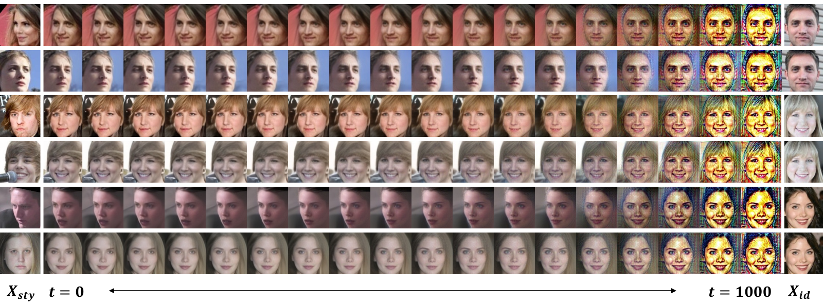
Fig. 5 shows how DDPM generates output at each time-step. The far left column shows $\bm{X}_{sty}$ , the desired style of an image. The far right column shows $\bm{X}_{id}$ , the desired ID image of choice. In early time-steps, the network reconstructs the front-view image with an ID of $\bm{X}_{id}$ . And gradually, it interpolates the image into the desired style of $\bm{X}_{sty}$ . The gradual transition can be in the pose, hair-style, expression, etc.

D.2 Interpolation

In Fig. 6, we show the plot of interpolation in $\bm{X}_{sty}$ . While keeping the same identity $\bm{X}_{id}$ , we take two style images $\bm{X}_{sty1}$ and $\bm{X}_{sty2}$ . We interpolate with $\alpha$ in $\alpha E_{stry}(\bm{X}_{sty1})+(1-\alpha)E_{stry}(\bm{X}_{sty2})$ with $\alpha$ increasing linearly from $0$ to $1$ . The interpolation is smooth, creating an intermediate pose and expression that did not exist before.

E Miscelaneous

Similarity threshold. Threshold=0.3 is based on FR evaluation model having a threshold of $0.3080$ for verification with TPR@FPR= $0.01\%:97.17$ % on IJB-B ijbb. FPR= $0.01\%$ is widely used in practice and the scale of similarity is $(\!-\!1\!,1\!)$ . At threshold=0.3, FFHQ has 200 (2%) more unique subjects than DDPM, signaling a similar level of uniqueness.

Style Extracting Model. We use the early layers of face recognition model for style extractor backbone. Our rationale for adopting the early layers of the FR model, as opposed to that of the ImageNet-trained model is that the early layers extract low-level features and we wanted features optimized with the face dataset. But, it is possible to take other models as long as it generates low-level features.

Evaluation on Harder Datasets. We evaluate on harder datasets, IJB-B ijbb (TPR@FPR=0.01%: $75.12$ ) and TinyFace tinyface (Rank1: $41.66$ ). We include this result for future works to evaluate on harder datasets.

Real and Generated Similarity Analysis. In addition to Fig.7 mathcing $\hat{X}_{id}$ with CASIA-WebFace, matching all $\hat{X_{0}}$ (generated) images against CASIA-WebFace at threshold=0.3, we get 0.0026% FMR. This implies that only a small fraction of CAISA-WebFace images are similar to the generated images.

F Societal Concerns

We believe that the Machine Learning and Computer Vision community should strive together to minimize the negative societal impact. Our work falls into the category of 1) image generation using generative models and 2) synthetic labeled dataset generation. In the field of image generation, unfortunately, there are numerous well-known malicious applications of generative models. Fake images can be used to impersonate high-profile figures and create fake news. Conditional image generation models make the malicious use cases easier to adapt to different use cases because of user controllability. Fortunately, GAN-based generators produce subtle artifacts in the generated samples that allow the visual forgery detection wang2020cnn; yu2019attributing; girish2021towards; proactive. With the recent advance in DDPM, the community is optimistic about detecting forgeries in diffusion models sha2022fake. It is also known that proactive treatments on generated images increase the forgery detection performance proactive, and as generative models become more sophisticated, proactive measures may be advised whenever possible.

Synthetic dataset generation is, on the other hand, an effort to avoid infringing the privacy of individuals on the web. Large-scale face dataset is collected without informed consent and only a few evaluation datasets such as IJB-S ijbs has IRB compliance for safe and ethical research. Collecting large-scale datasets with informed consent is prohibitively challenging and the community uses web-crawled datasets for the lack of an alternative option. Therefore, efforts to create synthetic datasets with synthetic subjects can be a practical solution to this problem. In our method, we still use real images to train the generative models. We hope that research in synthetic dataset generation will eventually replace real images, not just in the recognition task, but also in the generative tasks as well, removing the need for using real datasets in any form.

G Implementation Details and Code

The code will be released at https://github.com/mk-minchul/dcface. For preprocessing the training data CASIA-WebFace casia, we reference AdaFace kim2022adaface and use MTCNN zhang2016joint for alignment and cropping faces. For the backbone model definition, TFace TFace and for evaluation of LFW lfw, CFP-FP cfpfp, CPLFW cplfw, AgeDB agedb and CALFW calfw, we use AdaFace repository kim2022adaface.

DCFace: Synthetic Face Generation with Dual Condition Diffusion Model

Abstract

1 Introduction

2 Related Works

3 Proposed Approach

3.1 Preliminary

3.2 Dual Condition Generator Gm​i​xG_{mix}

3.3 Condition Sampling Strategy

4 Dataset Evaluation

5 Experiments

5.1 Model Ablation

5.2 Sampling Ablation

5.3 Comparison with Previous Methods

6 Conclusion

References

A Training Details

A.1 Architecture Detals

A.2 Training Hyper-Parameters

B More Experiment Results

B.1 Adding Real Dataset

B.2 Combining Multiple Synthetic Datasets

C Analysis

D Visualizations

D.1 Time-step Visualizaton

D.2 Interpolation

E Miscelaneous

F Societal Concerns

G Implementation Details and Code

3.2 Dual Condition Generator $G_{mix}$