One-dimensional pseudoharmonic oscillator: classical remarks and quantum-information theoryJournal: Journal of Physics Communications
Abstract
Motion along semi-infinite straight line in a potential that is a combination of positive quadratic and inverse quadratic functions of the position is considered with the emphasis on the analysis of its quantum-information properties. Classical measure of symmetry of the potential is proposed and its dependence on the particle energy and the factor describing a relative strength of its constituents is described; in particular, it is shown that a variation of the parameter alters the shape from the half-harmonic oscillator (HHO) at to the perfectly symmetric one of the double frequency oscillator (DFO) in the limit of huge . Quantum consideration focuses on the analysis of information-theoretical measures, such as standard deviations, Shannon, Rényi and Tsallis entropies together with Fisher information, Onicescu energy and non–Gaussianity. For doing this, among others, a method of calculating momentum waveforms is proposed that results in their analytic expressions in form of the confluent hypergeometric functions. Increasing parameter modifies the measures in such a way that they gradually transform into those corresponding to the DFO what, in particular, means that the lowest orbital saturates Heisenberg, Shannon, Rényi and Tsallis uncertainty relations with the corresponding position and momentum non–Gaussianities turning to zero. A simple expression is derived of the orbital-independent lower threshold of the semi-infinite range of the dimensionless Rényi/Tsallis coefficient where momentum components of these one-parameter entropies exist which shows that it varies between at HHO and zero when tends to infinity. Physical interpretation of obtained mathematical results is provided.
1 Introduction
It is well known [1, 2, 3, 4] that a three-dimensional (3D) spherically symmetric potential
| (1) |
written in position coordinates describes quite well roto-vibrational phenomena in diatomic molecules, with and being the dissociation energy between two atoms and equilibrium bond length, respectively. Its slightly amended 2D version
| (2) |
is indispensable in the analysis of the flat quantum rings [5, 6, 7, 8, 9, 10, 11, 12, 13, 14, 15]. Here, is a mass of the carrier, frequency defines a steepness of the confining in-plane outer surface of the annulus with its characteristic radius , and positive dimensionless constant describes a strength of the repulsive potential near the origin. 1D analogue of the above expressions for the straight motion along the positive semi-axis
| (3) |
was first introduced (with the simplifying assumption ) more than sixty years ago in a problem-solving textbook on quantum mechanics [16]. Despite of a such venerable age [17, 18, 19, 20, 21, 22, 23, 24, 25, 26, 27, 28, 29, 30, 31, 32, 33, 34], some properties of the movement in the similar type potentials that are commonly referred to as pseudoharmonic oscillator (PHO) still have not been addressed; namely, whereas quantum information measures, such as Shannon [35, 36], Rényi [37, 38] and Tsallis [39] entropies, Fisher information [40, 41], Onicescu energy [42], have recently been calculated for the 2D [14, 15] and 3D [4] PHO, their 1D counterparts still almost have not been tackled with: the only exception is the discussion of the position and momentum Shannon and position Fisher functionals for the half harmonic oscillator (HHO) [43], i.e., the structure with . The primary aim of the present exposition is to close this gap. Mentioned above measures play a very important role in quantum information theory and it is essential for everyone dealing with this subject to have (at least superficial) knowledge about them. Experimental advances in evaluating, e.g., the Shannon [44, 45] and Rényi [45, 46, 47, 48] entropies force the researchers to better understand their theoretical foundations what will facilitate an implementation of these quantities in quantum-information processing. From this point of view, a consideration of the relatively simple models that allow manageable analytic expressions for the above-mentioned functionals sheds new light on their properties and, accordingly, enriches our knowledge about them. The main focus of our research aims at the influence of the variation of the dimensionless coefficient on the classical and quantum properties of the structure. As shown below, the 1D geometry with the potential from equation (3) provides analytic dependencies of standard deviations on for any orbital in either position or momentum space whereas for the Fisher information it is done for the position component only with all other measures exhibiting evident formulas just for the ground-state position parts. A cornerstone result on which the whole subsequent analysis is based highlights that an alteration of the parameter transforms the shape described by equation (3) from the highly asymmetric potential at where the minimum of the HO with frequency serves simultaneously as its left infinitely high boundary to the symmetric with respect to its only extremum regular HO with the frequency – in the opposite limit of the very large . In this process, the lowest-energy waveforms in either space undergo transformation from non–Gaussian to Gaussian dependencies. Non–Gaussianity is an important property of the quantum systems that finds its applications, among others, in quantum-information protocols, such as, e.g., entanglement distillation and entanglement swapping [49]. To quantify it, below the measure based on the relative Shannon entropy [50, 51, 52, 53] is used and its components’ decaying at the huge is analyzed. Simultaneously, the non–Gaussianity based on the quantum von Neumann entropy is calculated and compared to its position and momentum counterparts. Since, at the same time, the HO ground level at saturates Heisenberg, Shannon, Rényi and Tsallis uncertainty relations, from fundamental point of view it is extremely important and instructive to track and describe the approach of the corresponding measures to their HO counterparts when, e.g., the product of the position and wave vector deviations or the sum of the corresponding Shannon parts come closer and closer to the basal limits of one half and , respectively. This is why below the main attention is devoted (but not limited) to the lowest-energy orbital.
Simultaneously with the vigorous research in the field, the leading Universities actively include quantum-information theory into their curricula [54, 55] and for other academical institutions it seems in the nearest future an inevitable but welcome reality [56] what forces the educators to seek didactic and methodological ways to discuss with the students physical and mathematical basics of the corresponding functionals. Lately, several such attempts aimed at the graduate and senior undergraduate level have been made [57, 58, 59, 60]. Postgraduate courses on a more general topic of ’the concept of information in physics’ are being offered not only to the physicists but to a wider audience of ”students of other natural sciences as well as mathematics, informatics, engineering, sociology, and philosophy” [61]. In this context, the present exposition might be considered as a continuation of those previous pedagogical efforts.
The outline of presentation is as follows. Before addressing quantum aspects, Sec. 2 that considers a classical motion shows that some quantities such as, e.g., periodic time, distance between the two turning points and average speed, stay unaffected by . The first of them is not influenced by the particle energy either what is a consequence of the fact that the two latter ones obey a square root dependence on . A classical measure of symmetry is proposed that is the ratio of the distances between the zero potential position and the left and right turning points, respectively. This quantity monotonically increases from zero for HHO to its asymptotic value of unity at the very large . Initial step of Sec. 3 describes quantized energy spectrum and the corresponding position waveforms, which are the eigen values and eigen vectors of the time-independent Schrödinger equation. Analytic method of calculating momentum functions is proposed and its advantages are discussed. All this knowledge serves as a foundation to the main part that copes with the miscellaneous functionals of the position and momentum densities and their dependence. Measures addressed are: standard deviations, Shannon, Rényi and Tsallis entropies, Fisher informations, Onicescu energies and non–Gaussianities. Since their physical significance is described in many sources, including pedagogical ones [57, 58, 59, 60, 62], they are only briefly considered. For the first four of them, the uncertainty relations between the position and wave vector components are known and, as shown below, for the ground level they saturate with the growth of since the squares of the corresponding waveforms come closer and closer to the Gaussian dependencies. Discussion of the momentum wave function that started in section 3.1 and revealed that its expression contains a finite sum of confluent hypergeometric functions is employed for a derivation of a simple formula for the lowest limit of the semi-infinite range of the Rényi and Tsallis coefficients where these momentum functionals make sense. Derived mathematical formulas received their physical interpretation; in particular, a special role of the HO is highlighted.
2 Potential profile and classical motion
Throughout the whole discussion, we will interchangeably use the energy and its quantum equivalent where the confining frequency, which in classical mechanics is determined by the force constant as , defines the length according to
| (4) |
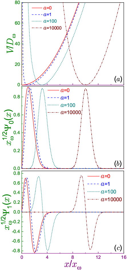
Figure 1(a) exhibits the shape of the potential profile, equation (3), for several parameters . Its zero minimum is achieved at
| (5) |
Around this only extremum, at the positive coefficient, , its behaviour is governed by the Taylor expansion:
| (6) | |||||
At , equation (3) describes the geometry of a particle confined to the right-hand half of the HO of the frequency . Increasing repulsive factor shifts the minimum of the potential to the right, as it follows from equation (5), simultaneously transforming it at the greater into the more symmetric shape: the leading term of equation (6) corresponds to the HO with frequency centered at with the influence of the subsequent items there decreasing in the limit .

Symmetrization of the potential with the growing is confirmed from the classical analysis; namely, for the particle with the energy , its motion is confined between the left and right turning points:
| (7) |
with the asymptotes:
| (8c) | ||||
As a measure of symmetry, one can use the ratio
| (9) |
with being the distances between the position of the minimum and right/left turning points:
| (10) |
Its limits are:
| (11) |
Vanishing ratio at tending to zero is naturally explained by the potential minimum in this regime moving closer and closer to the left turning point and actually merging with it for HHO, , whereas in the opposite limit of the huge parameter the zero-velocity positions are located almost symmetrically with respect to . On the other hand, since at the zero energy the particle does not move, both and are equal to what mathematically directly follows from equations (7) and (5), and, accordingly, the ratio of the two zero values of and yields the unity symmetry factor, . Dependence is depicted in figure 2. Observe that at any the symmetry decreases with the energy growing.
Closely related to the above topic is a concept of a periodic time which is a duration of a travel from, e.g., the left turning point towards its right counterpart, bouncing at it and a subsequent return to the initial position [63]:
| (12) |
where the argument at underlines that in general this quantity is a function of energy. Plugging in the 1D potential from equation (3) into this formula and calculating the integral with its limits from equation (7) yields:
| (13a) | ||||
| This result deserves some attention. First, it manifests that for our shape the periodic time does not depend on . Potentials obeying such condition are called isochronous [64]. It is known that to be isochronous, the potential needs to guarantee that its diameter should vary with energy as its square root [65]. Calculating with the help of equation (7), one elementary obtains that it is really the case for the PHO: | ||||
| (13b) | ||||
It was shown that a combination of the quadratic and inverse quadratic dependencies like the one from equation (3) (up to a shift and adding a constant) is the only 1D rational potential satisfying isochronous requirement [29]. Second, the diameter , equation (13b), and, as a consequence, the periodic time , equation (13a), of our system are not influenced by the parameter either and, moreover, they are equal to the one half of their HO counterparts with frequency :
| (14a) | ||||
| (14b) | ||||
in other words, regardless of the coefficient , the periodic time of the potential, equation (3), is equal to that of the HO with frequency . It is the easiest to explain these results in the limiting cases of the strong and weak ; e.g., for the HHO, , the distance traveled along one closed loop is precisely two times shorter than for the HO with the shape of the cut part being a mirror symmetric of that at what results in halving the time. Note that the average speed for both potentials is the same:
| (15) |
3 Quantum-information measures
3.1 Energy spectrum and position and momentum wave functions
A first step in the quantum analysis is a finding of the energies and position waveforms , , which are eigen values and eigen functions of the 1D Schrödinger equation:
| (16) |
For the -dependent potential from equation (3), they are:
| (17a) | ||||
| (17b) | ||||
Here, , is -function [66], is th order associated Laguerre polynomial [66], and the set at any parameter is orthonormalized:
| (18) |
, with being a Kronecker delta. In the limiting cases, the energy spectrum simplifies to:
at the small :
| (17a′) | ||||
| at the huge parameter: | ||||
| (17a′′) | ||||
Latter relation manifests that, as expected, the shift of the minimum to the right subdues the effect of the boundary what results in the gradual transformation of the potential to the HO shape with frequency . Observe that, according to equation (17a), the spectrum at any stays equidistant and the variation of this parameter from zero to the huge values shifts the energies downward by keeping the orbital-independent difference constant, . As it follows from equation (17b) and relation between Hermite and Laguerre polynomials [66], at the spatial dependence reads [43]:
| (17b′) |
and the corresponding eigen values are, according to equation (17a′), those of the -frequency HO with the odd indices only. Parts (b) and (c) of Figure 1, which depict waveforms of the ground- and first-excited orbitals, respectively, demonstrate that the increasing parameter transforms the function [] into the dependence that becomes more and more symmetric (anti symmetric) with respect to . Let us also note that the divergence of the potential from equation (3) at the left edge forces the function to vanish there at any and : , what is directly seen from solutions (17b) and (17b′) and is depicted in panels (b) and (c).

Momentum (or, more correctly, wave vector) dependencies are Fourier transforms of their position counterparts:
| (19) |
and as such they inherit the orthonormalization from equation (18):
| (20) |
Fourier transform that is inverse to equation (19) reads:
| (21) |
Substituting from equation (17b) into (19), one gets after elementary algebra:
| (22) |
with the integral here being essentially complex:
| (23) |
where both and are real and obey the even, , and odd, , symmetry, respectively. Unfortunately, there is no in the known literature [66, 67, 68] any relevant formula for the integral in equation (22). To deal with in our subsequent consideration, we found it convenient to use an explicit expression of the associated Laguerre polynomial in terms of powers of its argument [66]:
| (24) |
which, when substituted into equation (22), produces a finite sum of Weber parabolic cylinder functions [66] since their integral representation reads
| (25) |
Next, a splitting of the Weber function with purely imaginary argument into the real and imaginary parts [66] leads to the same result of the momentum dependence, equation (23); in particular, for the ground level one has:
| (26a) | ||||
| (26b) | ||||
where Kummer confluent hypergeometric functions [69] emerge since the parabolic cylinder functions are expressed with their help [66]. Figure 3 depicts dependencies from equations (26) at several . It is seen that the frequency of fading oscillations of the real and imaginary parts does increase at the growing parameter but, irrespective of it, the absolute value is a smooth monotonically decreasing to zero function of the magnitude of the wave vector with no nodes on the -axis. As was shown before [43], the real part of the HHO momentum dependence of any orbital is expressed with the help of the imaginary error function , with being error function [66] whereas is a polynomial of the degree multiplied by . In the opposite limit of the extremely huge , the asymptotic behaviour of the Kummer functions [66] yields:
| (27) |
where the last step in this chain elementary follows, according to equation (4), from the identity . Second exponent in the right-hand side of relation (27) explains the increase of the frequency of the fading oscillations with the unrestricted growth of whereas all remaining multipliers there represent the ground-state momentum waveform [57, 59, 62] of the HO with confining potential determined by . In a similar way, Kummer representation might be applied to the excited levels; for instance,
| (28a) | ||||
| (28b) | ||||
Then, as Figure 4 exemplifies, the even function exhibits two equal maxima located symmetrically with respect to the zero momentum whereas the minimum with the growth of the parameter decreases and at the huge is almost indistinguishable from zero with the whole shape approaching closer and closer its HO counterpart.


3.2 Standard deviations and Heisenberg uncertainty relation
Understanding of the position and momentum waveforms developed in the previous subsection paves the way to the analysis of the miscellaneous measures describing different facets of the particle localization/delocalization, oscillating structure of its distribution and its deviation from the uniformity in the corresponding domain. The most famous of them that is known to each undergraduate student [62] is a standard deviation that for the arbitrary 1D case has the following expression in the position and wave vector spaces:
| (29a) | ||||
| (29b) | ||||
where the brackets denote quantum expectation values of the operators or for the orbital with subscripts denoting the domain over which this averaging is calculated:
| (30a) | ||||
| (30b) | ||||
If the corresponding operators simplify to -numbers, i.e., and , then expressions (30) read:
| (31a) | ||||
| (31b) | ||||
and are the distribution densities:
| (32a) | ||||
| (32b) | ||||
Below, if the averaging domain is obvious, the subscript or will be dropped.
Standard deviations are quantitative measures of indeterminacy of the particle behaviour and as such describe the amount of information about its location () or motion () that is not known. The product of two satisfies the following inequality:
| (33) |
what is a mathematical expression of the celebrated Heisenberg uncertainty relation. It saturates for the HO ground state when the corresponding waveforms in either space are described by the Gaussian dependence [62]. Let us note that position (wave vector) component is measured in the units of length (inverse length) what makes equation (33) the most symmetric (and, accordingly, advantageous) compared to the use of the momentum instead of .
For PHO, the position mean value reads:
| (34) |
Here, is a generalized hypergeometric function [70]. In arriving at this relation, the value of the integral [67, 68]
has been used. It is worthwhile to point out that in equation (34) and majority of all other relations below the lengths are expressed in units of . In this way, at the huge the quantities take the values characteristic to HO. For the ground state, the above identity simplifies to
| (35a) | ||||
| and its asymptotic cases are: | ||||
| (35b) | ||||
| (35c) | ||||
Last equation shows that in the corresponding limit the function is localized around the minimum of the potential, as expected.
Expression takes a simple form for any orbital:
| (36) |
Accordingly, the ground-state position variance is calculated as
| (37a) | ||||
| with asymptotes | ||||
| (37b) | ||||
| (37c) | ||||
Here, and its square root that will be used below is .
In evaluating momentum variances and standard deviations, it has to be noticed first that, obviously, . For finding , one initially transforms it to averaging over the position space [62]:
| (38) |
with being a wave vector operator in -representation. Next, multiplying Schrödinger equation (16) by and integrating, the following relation is obtained:
| (39) |
Here,
| (40) |
Last expectation value in the right-hand side is calculated analytically [68]:
| (41) |
Ultimately,
| (42a) | ||||
| with asymptotes: | ||||
| (42b) | ||||
| (42c) | ||||
Then,
| (43) |
with .
Figure 5 shows evolution with of the ground-state dimensionless position and wave vector standard deviations together with their product. Both parts are monotonic functions of the parameter : position component grows from the above-mentioned HHO value of to the inverse square root of two at whereas its momentum counterpart decreases from at to for HO. This means that our knowledge about particle position (momentum) decreases (increases) with the enlarging . Momentum rate of change dominates over the position variation; as a result, the left-hand side of the Heisenberg inequality (33) monotonically gets smaller from the above-mentioned to the fundamental limit of one half that consists of the two equal contributions from and .
Let us finish this subsection by a brief note on the standard deviations of the excited states. It is known [62] that for the HO their position and wave vector components are and , respectively, with their product . Since at their variation with qualitatively reproduces their ground-orbital counterparts [what for, e.g., is directly seen from equations (42)], we do not plot them here.

3.3 Shannon quantum information entropies and non–Gaussianities
In general, for the motion in -dimensional space, Shannon position and wave vector entropies are defined as:
| (44a) | ||||
| (44b) | ||||
with and being the regions where the position and momentum densities, respectively, are defined with hyperindex counting the states in the increasing order of their energies. Two components of the Shannon quantum information entropy are not independent of each other but obey the inequality [71, 72]:
| (45) |
with . Similar to the quantities from the previous subsection, these measures quantify the amount of information that is not known but, compared to , they present a much more general base for defining ’uncertainty’ what, in particular, results in the fact that inequality (49) is much stronger than its Heisenberg fellow [73].
It is important to note that functionals from equations (44) present an extension to the continuous distributions of the entropy of a discrete case:
| (46) |
as was done already by C. E. Shannon himself [36]. Here, , , is a probability belonging to a discrete set of all (that might by finite or infinite) possible events, so that . This has several implications. First, contrary to the dimensionless , position and momentum entropies are measured in units of, respectively, positive and negative logarithm of length times dimensionality . Second, discrete Shannon entropy is never negative varying between zero (sure event, one of is equal to unity with all others disappearing) and (equiprobable situation, all happenings have the same chance to occur, ) whereas its continuous counterparts might fall below zero what takes place when the parts of the corresponding density, say, , which are larger than unity, in their contribution to the integral in equation (44a) overweigh those segments where . In this regard, it is important and instructive to point out that in equations (44) the classical rule from equation (46) is applied to the position and momentum spreadings of the pure state that is represented by the state vector. From this point of view, and should not be considered as ’quantum extensions’ of the quantities defined for classical dependencies but rather they are ’classical quantities’ applied to some quantum–related probability distributions. However, the most general quantum formulation employs the density operator suitable for the description of the mixed states. The corresponding von Neumann entropy
| (47) |
is non-negative and turns to zero for the pure state only. The distinction between quantum von Neumann entropy, equation (47), and components of the Shannon quantum–information entropy, equations (44), applies equally well for the Rényi and Tsallis measures considered in subsection 3.6.
For the system under consideration, equations (44) read:
| (48a) | ||||
| (48b) | ||||
and inequality (45) degenerates to
| (49) |
that is transformed into the identity for the Gaussian distributions, as it was the case for the standard deviations too. For the HO with its characteristic length , one has and .
As already stressed above, Shannon entropies of the continuous distributions from equations (48) are measured in units of the positive (position part) or negative (wave vector component) logarithm of the length. To avoid this physical ambiguity, in line with the previous discussions [74, 75], below the dimensionless quantities and are studied.
Due to the complicated form of the integrands in equations (48) for the excited orbitals, only ground-state position measure can be written analytically:
| (50a) | ||||
| is -function [66]. Limiting cases of equation (50a) are: | ||||
| (50b) | ||||
| (50c) | ||||
Here, is Euler’s constant [66], and . Leading term of right-hand side of equation (50b) does coincide with the HHO Shannon entropy [43]. All other position and momentum measures are calculated numerically only.
Ground-state dimensionless position and wave vector entropies together with their sum are shown in figure 6. The growth of decreases (increases) our knowledge about particle location (motion): position (wave vector) component monotonically gets bigger (smaller). Remarkably, the loss or gain of information is a purely quantum phenomenon: in classical picture, the diameter is not influenced by , as it follows from equation (13b). Similar to the standard deviations, section 3.2, momentum rate of change prevails over its position counterpart: as the potential with the enlarging shapes into the HO, the total unavailable information shrinks to the fundamental limit of approaching it from above with equal contribution from each item.
As was already stated several times, at large the ground orbital comes closer and closer to the Gaussian shape. To quantify the deviation from Gaussianity, we adapt for our geometry the measure introduced for the von Neumann entropy [50]; namely, position and momentum non–Gaussianities for the PHO read:
| (51a) | ||||
| (51b) | ||||
which are nothing else but relative entropies or Kullback–Leibler divergences [76]. Here, and are reference position and wave vector Gaussian states that have the same first and second position , and wave vector , moments, respectively, as the PHO ground level. Properties of the dimensionless functionals from equations (51) are very similar to those of the mixed states [50, 51]; in particular,
| (52) |
Their calculation is quite straightforward; for example, recalling that for the centered at the origin position HO with characteristic length the variance is , one equates it with its counterpart from equation (37a) finding in this way . Its knowledge effortlessly leads to the evaluation of the associated position entropy yielding ultimately:
| (53a) | ||||
| with the asymptotes: | ||||
| (53b) | ||||
| (53c) | ||||
Here, and . The sign of the last number shows that the position non–Gaussianity decreases at the small and equation (53c) expands this statement to the huge parameter. In a similar way, one finds the characteristic length of the reference momentum Gaussian state, which in general is different from its position fellow, and then evaluates the associated entropy:
| (54) |

Figure 7(a) shows evolution of both non–Gaussianities with the parameter . Either of them is a positive monotonically decreasing function of that tends to zero in the limit . For the HHO, momentum component with its value of is greater than its position counterpart but the magnitude of its speed of change at the small is faster and at it plunges below and stays much closer to zero. Interestingly, such asymptotic behaviour is opposite to that of the Shannon entropies, as a comparison between figures 6 and 7 reveals.
Having seen the evolution of and , which are ’classical’ measures of the quantum probability position and wave vector distributions, one might wonder how they match up with essentially quantum non–Gaussianity that for the single-mode orbitals reads [52]:
| (55a) | ||||
| and since for the pure states, which we only consider here, , this relation simplifies to: | ||||
| (55b) | ||||
with
| (56) |
Dimensionless elements of the (symmetric) covariance matrix
| are: | ||||
| (57c) | ||||
| (57d) | ||||
| (57e) | ||||
Similar to other 1D structures considered before [52], it is elementary to show that there are no correlations for our potential either what makes the covariance matrix a diagonal one, .
Panel (b) of figure 7 depicts the change of with . Similar to its position and momentum counterparts discussed above, it is a monotonically decreasing function of its argument being however, a few times greater than them; for example, close to the HHO, it behaves as
| (58a) | ||||
| and the coefficient at being negative: . In the opposite regime when the potential shape approaches the perfectly symmetric double frequency oscillator, the non–Gaussianity fades to zero according to: | ||||
| (58b) | ||||
Comparison of the latter relation with the position asympote from equation (53c) shows much slower wane of .

3.4 Fisher informations
Whereas Shannon entropy is a global measure of uncertainty, presence of the gradients and in the mathematical expressions of Fisher informations [40] makes them local indicators appraising the rates of change of the corresponding distribution:
| (59a) | ||||
| (59b) | ||||
These equations state that the steeper or more oscillatory the distribution is, the larger the corresponding Fisher term becomes. Avalanche-like growing diversity of applications of this quantity is reflected in a remarkable fact: first edition of book [41] was entitled ’Physics from Fisher information’ and in the later printings it has been changed to its present wording. Important for our consideration, one has to point out at the crucial role of this measure in building the bridge between the energy and information: it was shown that in density-functional theory its position component is nothing else than the functional of the kinetic energy of the many-particle system [77]. Contrary to the Shannon entropy, inequality (45), there is no similar universal relation between position and momentum components of the Fisher information. For the D Gaussian distribution with characteristic frequency , i.e., for the HO lowest-energy orbital, , dimensionless parts are equal to each other [78], as is the case with all other measures too:
| (60) |
For the 1D PHO, equations (59) become:
| (61a) | ||||
| (61b) | ||||
After straightforward [67, 68] but lengthy calculation, the position component takes the form:
| (62a) | ||||
| with the asymptotes: | ||||
| (62b) | ||||
| (62c) | ||||
In equation (62b), the leading term describes a contribution from the HHO [43].
Energy spectrum, equation (17a), and characteristics (62a) have many features in common: both are equidistant with linear dependence on quantum index, both are monotonically decreasing functions with almost coinciding shapes what can be, for example, seen from the same asymptotic behaviour at huge , cf. equations (17a′′) and (62c). This very close similarity is another exemplification of the intimate relation between the energy and position Fisher information whose curve is shown in figure 8: with the the increase of the parameter , from its value of it steadily approaches from above HO magnitude of two.
Momentum components are calculated numerically only. Dotted curve in figure 8 shows that its dependence grows with (as all other do too): for HHO, it is equal to whereas in the opposite regime it nears the value of the HO with frequency . Similar to its position counterpart, at any is an increasing function of the index. Note that at , position and wave vector parts are almost vertically symmetric with respect to line. As a result, their product in this range is practically indistinguishable from four, e. g., . For all other quantities studied here, the convergence of the combined measure is much slower.

3.5 Onicescu energies
Physically, Onicescu energies [42]
| (63a) | ||||
| (63b) | ||||
quantify a deviation of the corresponding distribution from the homogeneous one. This is easiest to show on the example of the function with compact support when the uniform distribution is just a constant that is an inverse of the corresponding volume, . Then, the global measure of the difference between any other dependence and its uniform fellow can be described by the quantity:
Elementary, one obtains:
| (64) |
Hence, the smaller the Onicescu energy is, the closer the corresponding density is to the uniform one.
As it follows from their definitions for the continuous functions, Onicescu energies are measured in units of the inverse volume of the corresponding domain; accordingly, they are not those energies that, e.g., are eigen values of the Schrödinger equation and measured in Joules. To underline the difference, the Romanian mathematician who proposed them for the discrete probabilities
| (65) |
used the term ’information energy’ [42]. Interchangeably and less confusing, they are also often called ’disequilibria’. Chronologically, it has to be mentioned that equation (65) has been used more than half a century before O. Onicescu [42] with a brief history described in ref. [79]. There is no known rigorous proof on the limits of the product of the position and wave vector components but apparently it should not exceed that of the HO:
| (66) |
with the equal HO contributions which for the ground orbital are:
| (67) |
For our system, disequilibria take the form:
| (68a) | ||||
| (68b) | ||||
with the ground-level position component being:
| (69a) | ||||
| with its limits: | ||||
| (69b) | ||||
| (69c) | ||||
Dashed line in figure 9 manifests that the increasing parameter makes the position density more homogeneous: the curve decreases from HHO value of to HO limit of . Simultaneously, wave vector component smoothly deviates from the uniformity: HHO magnitude of transforms at the huge parameter into its HO counterpart. Since the speed of change of is greater than the one of , combined position and momentum non-homogeneity gets stronger with . Qualitatively, the very similar dependencies are observed for other levels too when each component gets smaller for the higher lying states: , , what, of course, results in a similar behaviour of their product.
3.6 Rényi and Tsallis entropies
| (70a) | ||||
| (70b) | ||||
and Tsallis [39] (or, more correctly from a historical point of view, Havrda-Charvát-Daróczy-Patil-Taillie-Tsallis [80, 81, 82])
| (71a) | ||||
| (71b) | ||||
entropies with non-negative coefficient present one-parameter generalizations of the Shannon measure reducing to the latter in the limit :
| (72a) | ||||
| as can be easily established with the help of the l’Hôpital’s rule. Onicescu energy is their another particular case: | ||||
| (72b) | ||||
| Just second-order many-body Rényi entanglement entropy of an ensemble of triphenylphosphine molecules [45] and Bose-Einstein condensates of the interacting 87Rb atoms [46, 47] and 40Ca+ ions [48] was measured in recent cutting-edge experiments. In addition, Rényi and Tsallis entropies are expressed through each other as: | ||||
| (72c) | ||||
| (72d) | ||||
Physically, introduction of the parameter can be construed as a description of the deviation of the system from equilibrium and, then, these measures quantify the intensity of the response of the structure to this deflection. At the zero value of the Rényi/Tsallis coefficient, all random occurrences are treated on an equal footing, regardless of their actual happening, and in the opposite regime of the huge , the events with the highest probabilities are the only ones that contribute. As a result, both functionals and are monotonically decreasing functions of their parameter; e.g., at , the Rényi entropy (provided it does exist) is equal to the logarithm of the volume over which it is evaluated and at it is:
| (73) |
with the subscript in the right-hand side denoting a global maximum of the corresponding distribution. Fundamental difference between the two entropies is their treatment of the combined outcome of the two random events and ; namely, Rényi entropy is additive (or extensive):
| (74) |
what mathematically establishes the fact that the uncertainty of the happening is not influenced by the second set, if and are the two independent occurrences. Physically, equation (74) manifests that the total information acquired from the independent distributions is the sum of its counterparts for each of them. The concept of additivity was a cornerstone requirement for the Rényi search of the generalization of the Shannon entropy [37], which is extensive too:
| (75) |
Contrary, the Tsallis measure is only pseudo-additive:
| (76) |
It is known that momentum components are defined not on the whole non-negative semi-infinite axis (with the only exception of the HO) but this range is limited from below by the positive threshold [15, 59, 74, 75, 83, 84, 85]. This value is determined by the system geometry, its dimensionality [74, 83, 84, 85] and external influences, such as, e.g., electric or magnetic fields [15]. In addition, it might depend on the orbital itself [15, 85].
Sobolev inequality of the Fourier transform [86]
| (77) |
with the conjugation between and
| (78) |
straightforwardly leads to the Tsallis uncertainty relation [87]:
| (79) |
that in the neighbourhood of degenerates to [15]:
| (80) |
Here, is some characteristic length of the system (e.g., for our geometry, it is either or , as discussed above) and overlined quantities denote dimensionless Shannon entropies [75]:
| (81) |
Equation (80) immediately shows that the limit saturates Tsallis uncertainty relation what, of course, is also directly seen from equation (77). Besides, recalling inequality for the Shannon functionals, equation (45), one concludes that relation (80) is violated at ; hence, in addition to the conjugation from equation (78), Tsallis inequality (79) is valid in the range
| (82) |
only. Taking the logarithm of both sides of Sobolev inequality (77) yields the Rényi uncertainty relation [88, 89]:
| (83) |
simultaneously removing restriction (82). In the limit , it degenerates into its Shannon counterpart, equation (45). This is another manifestation of the differences between Rényi and Tsallis entropies. Uncertainty relations are an indispensable tool in data compression, quantum cryptography, entanglement witnessing, quantum metrology and other tasks employing correlations between the position and momentum components of the information measures [90, 91, 92, 93, 94, 95].
As it follows from equations (70), Rényi entropies, similar to the Shannon ones, are measured in units of the logarithm of the distance whereas the expressions of the Tsallis measures, equations (71), contain a dimensional incompatibility when the term of some power of length is subtracted from the unitless number. The reason of this ambiguity lies in the fact that definitions (70) and (71), similar to the Shannon entropy, were directly transferred to the continuous distributions from the discrete case where they are defined as:
| (84a) | ||||
| (84b) | ||||
Despite this incompatibility, Tsallis inequality (79) is dimensionally correct what, in particular, is exemplified by equation (80) with the use of conjugation (78):
| (85) |
Let us start our discussion of the 1D PHO from the dependence of the threshold coefficient on the parameter . For simplicity, consider the ground-state momentum Rényi entropy:
| (86) |
where, upon using the density , according to equations (32b) and (26), one has to evaluate the logarithm of the following integral:
| (87) |
To understand under which conditions this improper integral does converge, one employs asymptotic expansion of the Kummer confluent hypergeometric functions [66] to find out that at infinity both terms in integral (87) have the same dependence:
| (88a) | |||
| (88b) | |||
Accordingly, the integral will converge at what immediately leads to the following expression for the threshold:
| (89a) | ||||
| with asymptotes | ||||
| (89b) | ||||
| (89c) | ||||
It is easy to show that this fundamental relation is a level-independent one; indeed, at any , for example, the real part of the waveform will contain the sum of the functions with , what will result in the dependence at infinity. This, in turn, means that the term with will determine the overall convergence. Very similar reasoning applies to the imaginary parts too. Equations (89) promulgate that the HHO lower edge is equal to one quarter and, as the PHO coefficient grows, it decreases to zero when the potential takes the form of HO. As it is known [59], the HO is the only structure for which the momentum functional, similar to it position counterpart, exists at any non-negative . Obviously, the same conclusions apply to the Tsallis measures too.

Among many other properties of the 1D PHO entropies, we will discuss below the corresponding uncertainty relations. General Tsallis inequality (79) in our case reads:
| (90) |
where explicit expressions of the dimensionless position and momentum Tsallis components due to their unwieldiness are not written here. As already discussed above, this equation is dimensionally correct. Figure 10(a) shows and for HHO and . It confirms our earlier conclusion that the Tsallis inequality holds true only inside the range from equation (82) and it turns into the trivial identity at . Remarkably, the ground orbital saturates it at the opposite edge of one half too. This phenomenon was discovered before [15, 59, 74, 75, 83, 84] and its PHO explanation is very similar to other structures [15, 74, 75, 83, 84]; namely, at , left-hand side of relation (79) or, equivalently, (77), turns to
| (91) |
whereas in the right-hand one its coefficient tending to infinity picks up from the integral the maximum of the momentum waveform . Next, in equation (91) the absolute value of the function can be replaced by the function itself for the ground level only, , since is a sole position dependence that does not have nodes. Then, from the Fourier transform (19) one gets:
| (92) |
Zero wave vector is an extremum of the corresponding distribution for any orbital and, as figure 3 demonstrates, it is a global maximum of . This concludes a proof of the statement that at the ground state converts Tsallis relation into the identity. To develop it further, panel (b) plots the same dependencies for the first excited orbital. It shows that the corresponding curves intersect at only whereas at any smaller parameter, including the left edge of the interval (82), position part is strictly greater than the momentum component. In addition, it is important to point out that at the increasing PHO factor, the difference between and shrinks; for example, at , the designated lines are practically unresolved in the scale of panel (a). To elaborate on this, window (c) exhibits the difference
| (93) |
which monotonically dwindles unless at the infinitely large it turns to zero on the whole semi-axis : for the HO ground-state, irrespectively of the Tsallis coefficient, dimensionless part of each side is equal to with the constraint from requirement (82) being waived [59]. This is another manifestation of a special cachet of the Gaussian distribution [96].
Switching to the Rényi entropy again, let us note first that its ground-state position component is calculated analytically:
| (94a) | ||||
| For the vanishing coefficient, it reads: | ||||
| (94b) | ||||
| and for the infinite Rényi factor it is: | ||||
| (94c) | ||||
| Divergence at the zero , which in this regime does not depend on the PHO parameter, is explained by the semi-infinite range of integration. Relation (94c) was derived from equation (73) by zeroing first a derivative of the corresponding expression of and finding in this way the location of the maximum (note that at it approaches minimum of the potential, equation (5), as expected) and then substituting it back into . Also, in the limit Rényi entropy degenerates into its Shannon counterpart (50a): | ||||
| (94d) | ||||
| , , is a polygamma function [66], and at its exponent turns, according to relation (72b), into the Onicescu energy, equation (69a). Since the Rényi functional is a monotonically decreasing function of its parameter, expression in the square brackets in equation (94d) is negative at any what can be easily checked by direct calculation. It is also possible to derive the limiting cases of the potential; namely, near-HHO geometry yields | ||||
| (94e) | ||||
| and the functional approaches its HO counterpart [59] by obeying the rule: | ||||
| (94f) | ||||
In deriving the last dependence, a crucial role was played by Stirling’s formula [66]:
It is instructive to point out that the unit value of the Rényi parameter, , transforms equation (94f) into its Shannon simplification, equation (50c). The same is true about equations (94e) and (50b), respectively, where however, contrary to the previous link, the l’Hôpital’s rule is applied.

Figure 11(a) exhibits a dependence of the left-hand side of the ground-state Rényi uncertainty relation (83) in terms of the PHO and Rényi parameters. At any , this inequality turns into the identity at when its either part is equal to . Explanation of this is the same as for the Tsallis entropy presented above and is not discussed here. as a function of the coefficient possesses HHO broad maximum of located at approximately . As the potential shape changes, this maximum shrinks narrower simultaneously decreasing and shifting to the smaller until at the corresponding dependence turns to the HO one when the maximum of is located at the Shannon case [59]. For comparison, the HO dependence is shown by the black line at the front panel. To underline the convergence of the uncertainty relation (83) into the identity with the change of the shape, panel (b) depicts the difference between its left- and right-hand sides:
| (95) |
Of course, it is equal to zero at and any potential profile. It is seen also that at the difference get smaller with the increase of until at it identically turns to zero: for the HO, the ground-state uncertainty relation has its both sides equal to each other at any Rényi parameter [59].
4 Concluding remarks
Consideration of the models where a variation of one parameter leads to the change of the physical characteristics of the system enriches our knowledge from scientific and technological perspectives. One of such examples is introduced and scrutinized in the present research where a modification of the 1D potential profile is controlled by the dimensionless coefficient whose growth transforms asymmetric HHO into the regular HO with double frequency. Such evolution was investigated here with the emphasis on the analysis of quantum information measures. Some quantities, e.g., standard deviations and associated Heisenberg uncertainty relations or position components - either all, as for the Fisher information, or, at least, ground-state ones, as for the Shannon and Rényi entropies - allow analytic mathematical expressions whose asymptotes shed a bright light on the way they approach their HO counterparts. For the vast majority of the momentum components, numerical calculations are the only possible source of getting information but even here it has to be mentioned that a method was proposed for obtaining the analytic form of the corresponding waveforms what allowed, in particular, to derive a simple formula for the lower boundary that defines the range of the existence of the Rényi or Tsallis functionals. Exposition pays a large attention to the physical interpretation of the obtained results.
With contemporary nanotechnology advances, it is possible to grow quantum structures of any desired geometry. Accordingly, it should be no difficulty to build up 1D systems whose profile is described by equation (3) and to investigate their properties at different . Alternatively, at the fixed parameter one can vary the position of the minimum with respect to the left border by introducing an electric field directed along the axis what experimentally is achieved by, e.g., applying the appropriate gate voltage. Mathematically, an insertion of the item into the right-hand side of equation (3) modifies solutions of the Schrödinger equation: now they are expressed with the help of Heun functions [97, 98] - but physically its influence leads to the shift of the potential extremum away from the wall what results in the transformation of the structure into the 1D HO.
Finally, let us point out again that proposed here model of the modified PHO with its shape being controlled by the parameter has been widely used, as mentioned in the Introduction, in the analysis of the 2D quantum rings [5, 6, 7, 8, 9, 10, 11, 12, 13, 14, 15]. It is natural to expand such approach of investigating quantum-information concepts to any other dimension . For the 3D structure, the measures , , , and have been calculated at only [4] and for any higher dimensionality just energy spectrum and position wave functions have been analyzed [99, 100, 101, 102].
References
References
- [1] Davidson P M 1932 Eigenfunctions for calculating electronic vibrational intensities Proc. R. Soc. A 135 459–72
- [2] Sage M L 1984 The vibrations and rotations of the pseudogaussian oscillator Chem. Phys. 87 431–39
- [3] Oyewumi K J and Sen K D 2012 Exact solutions of the Schrödinger equation for the pseudoharmonic potential: an application to some diatomic molecules J. Math. Chem. 50 1039–59
- [4] Yahya W A, Oyewumi K J and Sen K D 2015 Position and momentum information-theoretic measures of the pseudoharmonic potential Int. J. Quantum Chem. 115 1543–52
- [5] Bogachek E N and Landman U 1995 Edge states, Aharonov–Bohm oscillations, and thermodynamic and spectral properties in a two–dimensional electron gas with an antidot Phys. Rev. B 52 14067–77
- [6] Tan W–C and Inkson J C 1996 Landau quantization and the Aharonov–Bohm effect in a two–dimensional ring Phys. Rev. B 53 6947–50
- [7] Tan W–C and Inkson J C 1996 Electron states in a two–dimensional ring – an exactly soluble model Semicond. Sci. Technol.11 1635–41
- [8] Tan W–C and Inkson J C 1999 Magnetization, persistent currents, and their relation in quantum rings and dots Phys. Rev. B 60 5626–35
- [9] Fukuyama H, Sasaki T, Yokoyama K and Ishikawa Y 2002 Orbital magnetism in confined two–dimensional systems J. Low Temp. Phys. 126 1067–80
- [10] Bulaev D V, GeylerV A and Margulis V A 2004 Effect of surface curvature on magnetic moment and persistent currents in two–dimensional quantum rings and dots Phys. Rev. B 69 195313
- [11] Simonin J, Proetto C R, Barticevic Z and Fuste G 2004 Single–particle electronic spectra of quantum rings: A comparative study Phys. Rev. B 70 205305
- [12] Olendski O and Barakat T 2014 Magnetic field control of the intraband optical absorption in two–dimensional quantum rings J. Appl. Phys.115 083710
- [13] Gumber S, Gambhir M, Jha P K and Mohan M 2016 Optical response of a two dimensional quantum ring in presence of Rashba spin orbit coupling J. Appl. Phys.119 073101
- [14] Olendski O 2019 Quantum information measures of the Aharonov-Bohm ring in uniform magnetic fields Phys. Lett. A 383 1110–22
- [15] Olendski O 2019 Rényi and Tsallis entropies of the Aharonov-Bohm ring in uniform magnetic fields Entropy 21 1060
- [16] Gol’dman L L and Krivchenkov V D 1961 Problems in Quantum Mechanics (London: Pergamon)
- [17] Weissman Y and Jortner J 1979 The isotonic oscillator Phys. Lett. A 70 177–9
- [18] Nieto M M and Simmons Jr. L M 1979 Coherent states for general potentials. II. Confining one-dimensional examples Phys. Rev. D 20 1332–41
- [19] Gutschick V P, Nieto M M, Simmons Jr. L M 1980 Coherent states for the ”isotonic oscillator” Phys. Lett. A 76 15–8
- [20] Weissman Y and Jortner J 1981 A comment on coherent states of the isotonic oscillator Phys. Lett. A 81 202
- [21] Nieto M M 1984 Resolution of the identity for minimum-uncertainty coherent states: An example related to charged-boson coherent states Phys. Rev. D 30 770–3
- [22] Sage M and Goodisman J 1985 Improving on the conventional presentation of molecular vibrations: Advantages of the pseudoharmonic potential and the direct construction of potential energy curves Am. J. Phys. 53 350–5
- [23] Ballhausen C J 1988 A note on the potential Chem. Phys. Lett. 146 449–51
- [24] Ballhausen C J 1989 ERRATUM: A note on the potential Chem. Phys. Lett. 154 174
- [25] Ballhausen C J 1988 Step-up and step-down operators for the pseudo-harmonic potential in one and two dimensions Chem. Phys. Lett. 151 428–30
- [26] Hall R L, Saad N and von Keviczky A B 1998 Matrix elements for a generalized spiked harmonic oscillator J. Math. Phys.39 6345–52
- [27] Crawford M G A 1999 The correspondence of two definitions of coherent states in a particular system J. Phys. A: Math. Gen.32 L215–9
- [28] Hall R L, Saad N and von Keviczky A B 2002 Spiked harmonic oscillators J. Math. Phys.43 94–112
- [29] Chalykh O A and Veselov A P 2005 A remark on rational isochronous potentials J. Nonlinear Math. Phys. 12 (Suppl 1) 179–83
- [30] Dong S–H, Lozada–Cassou M, Yu J, Jiménez–Ángeles F and Rivera A L 2007 Hidden symmetries and thermodynamic properties for a harmonic oscillator plus an inverse square potential Int. J. Quantum Chem. 107 336–71
- [31] Dong S–H 2007 Factorization Method in Quantum Mechanics (Dordrecht: Springer)
- [32] Tavassoly M K and Jalali H R 2013 Barut–Girardello and Gilmore–Perelomov coherent states for pseudoharmonic oscillators and their nonclassical properties: Factorization method \CPB22 084202
- [33] Mikulski D, Eder K and Molski M 2014 The algebraic approach for the derivation of ladder operators and coherent states for the Goldman and Krivchenkov oscillator by the use of supersymmetric quantum mechanics J. Math. Chem. 52 1610–23
- [34] Baykal M and Baykal A 2022 The pseudoharmonic oscillator energy spectrum Eur. J. Phys.43 035406
- [35] Shannon C E 1948 A mathematical theory of communication Bell Syst. Tech. J. 27 379–423
- [36] Shannon C E 1948 A mathematical theory of communication. Part III. Mathematical preliminaries Bell Syst. Tech. J. 27 623–56
- [37] Rényi A 1960 On measures of information theory Proceedings of the Fourth Berkeley Symposium on Mathematics, Statistics and Probability (Berkeley University Press: Berkeley, CA, USA)
- [38] Rényi A 1970 Probability Theory (Amsterdam: North-Holland)
- [39] Tsallis C 1988 Possible generalization of Boltzmann-Gibbs statistics J. Stat. Phys. 52 479–87
- [40] Fisher R A 1925 Theory of statistical estimation Math. Proc. Cambridge Philos. Soc. 22 700–25
- [41] Frieden B R 2004 Science from Fisher Information (Cambridge: Cambridge)
- [42] Onicescu O 1966 Énergie informationnelle C. R. Acad. Sci. Ser. A 263 841–2
- [43] Shi Y–J, Sun G–H, Jing J and Dong S–H 2017 Shannon and Fisher entropy measures for a parity-restricted harmonic oscillator Laser Phys. 27 125201
- [44] Lukin A, Rispoli M, Schittko R, Tai M E, Kaufman A M, Choi S, Khemani V, Leonard J and Greiner M 2019 Probing entanglement in a many–body–localized system Science 364 256–60
- [45] Niknam M, Santos L F and Cory D G 2021 Experimental detection of the correlation Rényi entropy in the central spin model Phys. Rev. Lett.127 080401
- [46] Islam R, Ma R, Preiss P M, Tai M E, Lukin A, Rispoli M and Greiner M 2015 Measuring entanglement entropy in a quantum many-body system Nature (London) 528 77–83
- [47] Kaufman A M, Tai M E, Lukin A, Rispoli M, Schittko R, Preiss P M and Greiner M 2016 Quantum thermalization through entanglement in an isolated many–body system Science 353 794–800
- [48] Brydges T, Elben A, Jurcevic P, Vermersch B, Maier C, Lanyon B P, Zoller P, Blatt R and Roos C F 2019 Probing Rényi entanglement entropy via randomized measurements Science 364 260–3
- [49] Walschaers M 2021 Non–Gaussian quantum states and where to find them PRX Quantum 2 030204
- [50] Genoni M G, Paris M G A and Banaszek K 2008 Quantifying the non–Gaussian character of a quantum state by quantum relative entropy Phys. Rev. A 78 060303
- [51] Genoni M G and Paris M G A 2010 Quantifying non–Gaussianity for quantum information Phys. Rev. A 82 052341
- [52] Paris M G A, Genoni M G, Shammah N and Teklu B 2014 Quantifying the nonlinearity of a quantum oscillator Phys. Rev. A 90 012104
- [53] Albarelli F, Genoni M G, Paris M G A and Ferraro A 2018 Resource theory of quantum non–Gaussianity and Wigner negativity Phys. Rev. A 98 052350
- [54] Aiello C D et. al. 2021 Achieving a quantum smart workforce Quantum Sci. Technol. 6 030501
- [55] Cervantes B, Passante G, Wilcox B and Pollock S 2021 An Overview of Quantum Information Science Courses at US Institutions Physics Education Research Conference Proceedings pp. 93–98 (edited by M B Bennett, B W Frank and R Vieyra)
- [56] Fox M F J, Zwickl B M and Lewandowski H J 2020 Preparing for the quantum revolution: What is the role of higher education? Phys. Rev. Phys. Educ. Res. 16 020131
- [57] Saha A, Talukdar B and Chatterjee S 2017 On the realization of quantum Fisher information Eur. J. Phys.38 025103
- [58] Olendski O 2017 Comment on ’On the realisation of quantum Fisher information’ Eur. J. Phys.38 038001
- [59] Olendski O 2019 Rényi and Tsallis entropies: three analytic examples Eur. J. Phys.40 025402
- [60] Nascimento W S, de Almeida M M and Prudente F V 2020 Information and quantum theories: an analysis in one–dimensional systems Eur. J. Phys.41 025405
- [61] Dittrich T 2015 ’The concept of information in physics’: an interdisciplinary topical lecture Eur. J. Phys.36 015010
- [62] Griffiths D J 2018 Introduction to Quantum Mechanics (Non-Relativistic Theory) 3rd ed. (Cambridge: Cambridge University Press)
- [63] Landau L D and Lifshitz E M 1976 Mechanics (New York: Pergamon)
- [64] Calogero F 2008 Isochronous Systems (New York: Oxford)
- [65] Pippard A B 1989 The Physics of Vibration (New York: Cambridge)
- [66] Abramowitz M and Stegun I A 1964 Handbook of Mathematical Functions (New York: Dover)
- [67] Gradshteyn I S and Ryzhik I M 2014 Tables of Integrals, Series, and Products 8th ed. (New York: Academic Press)
- [68] Prudnikov A P, Brychkov Y A and Marichev O I 1992 Integrals and Series vol. 2 (New York: Gordon and Breach)
- [69] Mathews W N Jr, Esrick M A, Teoh Z Y and Freericks J K 2022 A physicist’s guide to the solution of Kummer’s equation and confluent hypergeometric functions Condens. Matter Phys. 25 33203
- [70] Bailey W N 1935 Generalised Hypergeometric Series (Cambridge: Cambridge University Press)
- [71] Białynicki-Birula I and Mycielski J 1975 Uncertainty relations for information entropy in wave mechanics Commun. Math. Phys. 44 129–32
- [72] Beckner W 1975 Inequalities in Fourier analysis Annals Math. 102 159–82
- [73] Deutsch D 1983 Uncertainty in Quantum Measurements Phys. Rev. Lett.50 631–3
- [74] Olendski O 2021 Quantum information measures of the Dirichlet and Neumann hyperspherical dots Eur. Phys. J. Plus 136 390
- [75] Olendski O 2022 Quantum-information theory of a Dirichlet ring with Aharonov-Bohm field Eur. Phys. J. Plus 137 451
- [76] Kullback S and Leibler R A 1951 On information and sufficiency Annals Math. Stat. 22 79–86
- [77] Sears S B, Parr R B and Dinur U 1980 On the quantum–mechanical kinetic energy as a measure of the information in a distribution Israel J. Chem. 19 165–73
- [78] Dehesa J S and Toranzo I V 2020 Dispersion and entropy–like measures of multidimensional harmonic systems: application to Rydberg states and high–dimensional oscillators Eur. Phys. J. Plus 135 721
- [79] Ellerman D 2009 Counting distinctions: on the conceptual foundations of Shannon’s information theory Synthese 168 119–49
- [80] Havrda J and Charvát F 1967 Quantification method of classification processes. Concept of structural a-entropy Kybernetika 3 30–5
- [81] Daróczy Z 1970 Generalized information functions Inform. Control 16 36–51
- [82] Patil G P and Taillie C 1982 Diversity as a concept and its measurement J. Am. Stat. Assoc. 77 548–61
- [83] Olendski O 2020 Rényi and Tsallis entropies of the Dirichlet and Neumann one–dimensional quantum wells Int. J. Quantum Chem. 120 e26220
- [84] Olendski O 2021 Comparative analysis of information measures of the Dirichlet and Neumann two–dimensional quantum dots Int. J. Quantum Chem. 121 e26455
- [85] Aptekarev A I, Belega E D and Dehesa J S 2021 Rydberg multidimensional states: Rényi and Shannon entropies in momentum space \jpa54 035305
- [86] Beckner W 1975 Inequalities in Fourier analysis on P. Natl. Acad. Sci. USA 72 638–41
- [87] Rajagopal A K 1995 The Sobolev inequality and the Tsallis entropic uncertainty relation Phys. Lett. A 205 32–6
- [88] Białynicki-Birula I 2006 Formulation of the uncertainty relations in terms of the Rényi entropies Phys. Rev. A 74 052101
- [89] Zozor S and Vignat C 2007 On classes of non–Gaussian asymptotic minimizers in entropic uncertainty principles Physica A 375 499–517
- [90] Wehner S and Winter A 2010 Entropic uncertainty relations – a survey New J. Phys.12 025009
- [91] Jizba P, Dunningham J A and Joo J 2015 Role of information theoretic uncertainty relations in quantum theory Ann. Phys., NY355 87–115
- [92] Coles P J, Berta M, Tomamichel M and Wehner S 2017 Entropic uncertainty relations and their applications Rev. Mod. Phys.89 015002
- [93] Toscano F, Tasca D S, Rudnicki Ł and Walborn S P 2018 Uncertainty relations for coarse–grained measurements: an overview Entropy 20 454
- [94] Hertz A and Cerf N J 2019 Continuous-variable entropic uncertainty relations \jpa52 173001
- [95] Wang D, Ming F, Hu M-L and Ye L 2019 Quantum–memory–assisted entropic uncertainty relations Ann. Phys. (Berlin) 531 1900124
- [96] De Palma G, Trevisan D, Giovannetti V and Ambrosio L 2018 Gaussian optimizers for entropic inequalities in quantum information J. Math. Phys.59 081101
- [97] Ronveaux A and Arscott F M (eds) 1995 Heun’s differential equations (Oxford: Oxford University Press)
- [98] Hortaçsu M 2018 Heun functions and some of their applications in physics Adv. High Energy Phys. 2018 8621573
- [99] Wang L-Y, Gu X-Y, Ma Z-Q and Dong S-H 2002 Exact solutions to –dimensional Schrödinger equation with a pseudoharmonic oscillator Found. Phys. Lett. 15 569–76
- [100] Oyewumi K J and Bangudu E A 2003 Isotropic harmonic oscillator plus inverse quadratic potential in -dimensional spaces Arab. J. Sci. Eng. 28 173–82
- [101] Oyewumi K J, Akinpelu F O and Agboọla A D 2008 Exactly complete solutions of the pseudoharmonic potential in –dimensions Int. J. Theor. Phys. 47 1039–57
- [102] Das T and Arda A 2015 Exact analytical solution of the –dimensional radial Schrödinger equation with pseudoharmonic potential via Laplace transform approach Adv. High Energy Phys. 2015 137038