跳到论文正文
W Papers独立论文阅读器 arXiv:2304.06326 论文正文 计算阅读时间 · 0%
引用这篇论文根据当前论文元数据生成,正式投稿前建议核对。


License: arXiv.org perpetual non-exclusive license
arXiv:2304.06326v2 [stat.ML] 19 Apr 2023

Understanding Overfitting in Adversarial Training via Kernel Regression

Teng Zhang Email: teng.zhang@ucf.edu Thanks: Department of Mathematics, Univerisity of Central Florida, Orlando, FL ().    Kang Li Email: kang.li@ucf.edu Thanks: Department of Mathematics, Univerisity of Central Florida, Orlando, FL ()
Abstract

Adversarial training and data augmentation with noise are widely adopted techniques to enhance the performance of neural networks. This paper investigates adversarial training and data augmentation with noise in the context of regularized regression in a reproducing kernel Hilbert space (RKHS). We establish the limiting formula for these techniques as the attack and noise size, as well as the regularization parameter, tend to zero. Based on this limiting formula, we analyze specific scenarios and demonstrate that, without appropriate regularization, these two methods may have larger generalization error and Lipschitz constant than standard kernel regression. However, by selecting the appropriate regularization parameter, these two methods can outperform standard kernel regression and achieve smaller generalization error and Lipschitz constant. These findings support the empirical observations that adversarial training can lead to overfitting, and appropriate regularization methods, such as early stopping, can alleviate this issue.

keywords
kernel regression, adversarial training, data augmentation, overfitting
††runningheads: Understanding Overfitting in Adversarial Training / T. Zhang and K. Li
MSC
62J07, 46E22, 65F22

1 Introduction

Over the past decade, deep learning, a subfield of artificial intelligence that utilizes neural network-based models, has undergone a major transformation, leading to significant advancements in various domains such as computer vision, speech recognition, and robotics [20]. As a result, a substantial body of research has emerged aimed at explaining the mathematical foundations of deep learning’s success [3, 2, 43, 42, 15, 29, 56, 16, 5].

Recent studies have demonstrated that neural network models, despite achieving human-level performance on many important tasks, are not robust to adversarial examples—a small and human imperceptible input perturbation can easily change the prediction label. In light of the vulnerability of standard neural network algorithms to adversarial attacks, several algorithms have been proposed that aim to provide resilience to such attacks [41, 49, 40, 50, 39, 10, 34, 7, 48, 27, 59, 38, 47, 35, 54]. For example, adversarial training [47, 35] involves incorporating the generation of adversarial examples into the training process in order to improve the worst-case performance of the model. However, the theoretical foundations of these robust algorithms are not well understood, and adversarial training can present practical challenges such as implicit bias [31] and overfitting [46]. Regularization techniques, such as early stopping, have been employed to mitigate the overfitting issue [12], but the underlying mechanism is unclear.

This research aims to investigate the overfitting problem in adversarial training from a theoretical perspective and explains why regularization techniques can be used to mitigate it. Motivated by the observation that neural networks can be approximated with neural tangent kernel regression [24, 19], we analyze adversarial training and data augmentation with noise in the context of kernel regression in reproducing kernel Hilbert space (RKHS). The present study contributes to the field by:

  • •

    Establishing the limiting formula for adversarial training and data augmentation with noise as the regularization parameter and the size of the attack or noise approach zero.

  • •

    Demonstrating that in comparison with standard kernel regression, adversarial training and data augmentation without regularization have greater generalization error and Lipschitz constant, whereas adversarial training and data augmentation with suitable regularization have lower generalization error and Lipschitz constant.

  • •

    Verifying theoretical findings by experiments on artificial and real data sets.

Our theoretical analysis, in conjunction with the neural tangent kernel, provides a first explanation as to why adversarial training tends to exhibit overfitting, and why regularization techniques are effective in mitigating this issue.

1.1 Existing works

This section presents a comprehensive review of the key developments in the field of neural network-based machine learning, with an emphasis on the tools and results that are relevant to our proposed research.

A Mathematical Understanding of Neural Network-Based Machine Learning Neural network-based models have become increasingly popular for addressing the problem of supervised learning, where a training dataset S=(𝐱i,yi)i=1n⊂ℝd×ℝS={(\mathbf{x}_{i},y_{i})}_{i=1}^{n}\subset\mathbb{R}^{d}\times\mathbb{R} is provided and the goal is to find a model f^:ℝd→ℝ\hat{f}:\mathbb{R}^{d}\rightarrow\mathbb{R} that generalizes well, meaning that f^​(𝐱)\hat{f}(\mathbf{x}) provides accurate predictions of yy on subsequent (𝐱,y)(\mathbf{x},y) pairs. A commonly used measure to measure the goodness of f^\hat{f} is the generalization error ℒ⁡(f)=Expect(𝐱,y)​l​(f⁡(𝐱),y){\mathcal{L}}(f)=\mathrm{Expect}_{(\mathbf{x},y)}l(f(\mathbf{x}),y), where ll is a suitable loss function such as the squared loss.

In neural network-based machine learning, the model f^\hat{f} is selected from a family of highly nonlinear statistical models. As a prototypical example, the feed-forward neural network with LL layer can be parametrized as f⁡(𝐱,θ)f(\mathbf{x};\mathbf{\theta}) by f(𝐱;θ)=σL(𝐖LσL1(𝐖L−1⋯σ1(𝐖1𝐱))),f(\mathbf{x};\mathbf{\theta})=\sigma_{L}(\mathbf{W}_{L}\sigma_{L_{1}}(\mathbf{W}_{L-1}\cdots\sigma_{1}(\mathbf{W}_{1}\mathbf{x}))), where θ=(𝐖1,⋯,𝐖L)\mathbf{\theta}=(\mathbf{W}_{1},\cdots,\mathbf{W}_{L}) in the set of parameters with 𝐖l∈ℝdl×dl−1\mathbf{W}_{l}\in{\mathbb{R}}^{d_{l}\times d_{l-1}}, and σl:ℝdl→ℝdl−1\sigma_{l}:{\mathbb{R}}^{d_{l}}\rightarrow{\mathbb{R}}^{d_{l-1}} are nonlinear activation functions. In practice, the fitted function f^\hat{f}, parameterized by f⁡(𝐱,θ^)f(\mathbf{x};\hat{\theta}), is usually chosen by minimizing the empirical risk function

ℒn​(θ)=1n​∑i=1nl⁡(yi,f⁡(𝐱i,θ)){\mathcal{L}}_{n}(\mathbf{\theta})=\frac{1}{n}\sum_{i=1}^{n}l(y_{i},f(\mathbf{x}_{i};\mathbf{\theta})) (1)

through gradient descent or stochastic gradient descent.

Tangent kernel of neural networks The neural tangent kernel (NTK) is a valuable instrument for comprehending neural network training and implicit regularization in gradient descent. It is shown that the evolution of neural networks during their training by gradient descent can be described using kernel regression with the neural tangent kernel (NTK) [25, 15, 1]. In particular, in any model that ff can be parameterized by f⁡(⋅,θ)f(\cdot,\theta) with θ∈ℝm\theta\in{\mathbb{R}}^{m}, the NTK kernel KK is defined by

K⁡(𝐱,𝐲)=∑i=1m∂θif⁡(𝐱,θ)​∂θif⁡(𝐲,θ).K(\mathbf{x},\mathbf{y})=\sum_{i=1}^{m}\partial_{\theta_{i}}f(\mathbf{x};\theta)\partial_{\theta_{i}}f(\mathbf{y};\theta). (2)

It is shown that as the width of a network goes to infinity, the gradient algorithm that minimizes (1) can be approximated with regression in reproducing kernel Hilbert space (RKHS) with the neural tangent kernel in (2) [24].

Adversarial training Considering that it has been observed that neural network-based algorithm are vulnerable to attacks, there have been numerous works that attempt to locate such adversarial example when the model is given, and on the other hand, develop robust deep learning algorithms.

In general, a defense mechanism called adversarial training [22, 36] generates robust algorithms by modifying the objective function that considers the worst-case perturbations and taking the gradient descent steps at (approximate) worst-case perturbations [21, 28, 36], or by using provably upper bound inner maximization [52, 37, 44, 13]. For example, instead of minimizing the standard objective function (1), these works minimize a modified objective function

ℒn(a​d​v)​(θ)=1n​∑i=1nmaxδ∈𝚫⁡l⁡(yi,f⁡(𝐱i+δ,θ)),{\mathcal{L}}_{n}^{(adv)}(\mathbf{\theta})=\frac{1}{n}\sum_{i=1}^{n}\max_{\mathbf{\delta}\in\mathbf{\Delta}}l(y_{i},f(\mathbf{x}_{i}+\mathbf{\delta};\mathbf{\theta})), (3)

where 𝚫\mathbf{\Delta} is the set of perturbations, such as 𝚫={𝚫:‖𝚫‖≤ϵ}\mathbf{\Delta}=\{\mathbf{\Delta}:\|\mathbf{\Delta}\|\leq\epsilon\}. In terms of implementation, [19, 58] show that in the over-parameterized regime, a heuristic form of robust optimization that alternates between minimization and maximization steps converges to a solution where the training error is within ϵ\epsilon of the optimal robust loss. However, it is unclear whether this algorithm can achieve a low generalization error.

Data augmentation Another commonly used strategy for improving robustness applies the technique of data augmentation [51, 53], which enhances the size of the training datasets by adding noises or attacks artificially and minimize

ℒn(a​u​g)​(θ)=1n​∑i=1nAverageδ∈𝚫​l​(yi,f⁡(𝐱i+δ,θ)),{\mathcal{L}}_{n}^{(aug)}(\mathbf{\theta})=\frac{1}{n}\sum_{i=1}^{n}\mathrm{Average}_{\mathbf{\delta}\in\mathbf{\Delta}}l(y_{i},f(\mathbf{x}_{i}+\mathbf{\delta};\mathbf{\theta})), (4)

where 𝚫\mathbf{\Delta} is the set of noises or attacks. As pointed out by Goodfellow et al. in [20, Section 7.4-7.5], injecting noise in the input to a neural network is a form of data augmentation, and can be considered as a regularization strategy.Empirical studies [45] verify its effectiveness in increasing the robustness of deep neural network methods.

Existing theories for adversarial learning and data augmentation While the adversarial training method has been popular, there has only been a few theoretical studies on it. Li et al. [31] shows that the implicit bias of gradient descent-based adversarial training promotes robustness against adversarial perturbation. For the basic setting of linear regression, Javanmard et al. [26] precisely characterize the standard and robust accuracy and the corresponding tradeoff achieved by a contemporary mini-max adversarial training approach in a high-dimensional regime where the number of data points and the parameters of the model grow in proportion to each other. However, the generalization to nonlinear kernels is not considered in this work. [55] studies adversarial learning, but only in the setting of a few learning algorithms such as kk-nn.

The theoretical analysis of data augmentation with noise is also quite lacking and existing works mostly focus on a few specific settings. Chen et al. [11] develop a framework to explain data augmentation as averaging over the orbits of the group that keeps the data distribution approximately invariant, and show that it leads to variance reduction. However, this analysis does not apply to the “noise injection” approach. Dao et al. [14] use the connection between data augmentation and kernel classifiers to show that a kernel classifier on augmented data approximately decomposes into two components: (i) an averaged version of the transformed features, and (ii) a data-dependent variance regularization term. This suggests that data augmentation improves generalization both by inducing invariance and by reducing model complexity. Hanin and Sun [23] analyze the effect of augmentation on optimization in the simple convex setting of linear regression with MSE loss, and interpret augmented (S)GD as a stochastic optimization method for a time-varying sequence of proxy losses.

Overfitting in adversarial neural network framework It has been observed for adversarial deep learning, overfitting to the training set does in fact harm robust performance to a very large degree in adversarially robust training across multiple datasets [46]: after a certain point in adversarial training, further training will continue to substantially decrease the robust training loss while increasing the robust test loss. In practice, regularization techniques such as early stopping can mitigate the overfitting problem [31]. However, the justification for overfitting in adversarial learning is missing. Interestingly, this is different from the traditional neural networks, where overfitting does not harm the performance [57, 4, 32], and it has been theoretically justified in some settings [17, 9].

1.2 Outline of the paper

The paper is organized as follows. Section 2 presents an introduction to the background and the problem setup that is being considered in this research. Section 3 provides a rigorous derivation of the limiting formula for the data augmented and adversarial estimators. Section 4 examines several scenarios and demonstrates that, in these cases, the ridgeless versions of these estimators exhibit overfitting behavior, as measured by both the generalization error and the Lipschitz constant, and the overfiting behavior can be ameliorated by regularization techniques. Section 5 verifies this phenomenon using both artificial and real data sets.

2 Background

This work studies the problem of supervised learning: assume nn i.i.d. observed pairs (𝐱i,yi)(\mathbf{x}_{i},y_{i}), 1≤i≤n1\leq i\leq n, drawn from an unknown probability distribution μ⁡(𝐱,y)\mu(\mathbf{x},y), and f∗f^{*} is the conditional expectation function f∗​(𝐱)=Expect⁡(y|𝐱=𝐱)f^{*}(\mathbf{x})=\mathrm{Expect}(y|\mathbf{x}=\mathbf{x}), then we aim to find ff such that the generalization risk

ℒ⁡(f)=Expect𝐱∼μ​(f⁡(𝐱)−f∗​(𝐱))2{\mathcal{L}}({f})=\mathrm{Expect}_{\mathbf{x}\sim\mu}({f}(\mathbf{x})-f^{*}(\mathbf{x}))^{2}

is as small as possible.

The supervised learning framework finds the function f∗f^{*} from a set ℋ\mathcal{H}, and here we consider the setting where ℋ\mathcal{H} is a reproducing kernel Hilbert space (RKHS), a set of functions ℝp→ℝ{\mathbb{R}}^{p}\rightarrow{\mathbb{R}} that is associated with a positive definite kernel K⁡(⋅,⋅):ℝp×ℝp→ℝK(\cdot,\cdot):{\mathbb{R}}^{p}\times{\mathbb{R}}^{p}\rightarrow{\mathbb{R}} and endowed with the norm ∥⋅∥ℋ\|\cdot\|_{{\cal H}}. Then we consider the standard estimator (1), with an additional ridge regularization term λ​‖f‖ℋ2\lambda\|f\|_{{\cal H}}^{2} that is commonly used in regression in RKHS:

f^λ\displaystyle\hat{f}_{\lambda} =argminf∈ℋ​ℒ^λ​(f),where​ℒ^λ(a​d​v)​(f)=1n​∑i=1n(yi−f⁡(𝐱i))2+λ​‖f‖ℋ2.\displaystyle=\mbox{argmin}_{f\in{\cal H}}\hat{{\mathcal{L}}}_{\lambda}(f),\,\,\,\text{where}\,\,\,\hat{{\mathcal{L}}}^{(adv)}_{\lambda}(f)=\frac{1}{n}\sum_{i=1}^{n}(y_{i}-f(\mathbf{x}_{i}))^{2}+\lambda\|f\|_{{\cal H}}^{2}. (5)

In addition, we consider the adversarial estimator (3) and the estimator with data augmentation (4) in the setting of RKHS, also with additional regularization:

f^λ(a​d​v)\displaystyle\hat{f}_{\lambda}^{(adv)} =argminf∈ℋ​ℒ^λ(a​d​v)​(f),where​ℒ^λ(a​d​v)​(f)=1n​∑i=1nmaxδ∈𝚫⁡(yi−f⁡(𝐱+δ))2+λ​‖f‖ℋ2,\displaystyle=\mbox{argmin}_{f\in{\cal H}}\hat{{\mathcal{L}}}^{(adv)}_{\lambda}(f),\,\,\,\text{where}\,\,\,\hat{{\mathcal{L}}}^{(adv)}_{\lambda}(f)=\frac{1}{n}\sum_{i=1}^{n}\max_{\mathbf{\delta}\in\mathbf{\Delta}}(y_{i}-f(\mathbf{x}+\mathbf{\delta}))^{2}+\lambda\|f\|_{{\cal H}}^{2}, (6)
f^λ(a​u​g)\displaystyle\hat{f}_{\lambda}^{(aug)} =argminf∈ℋ​ℒ^λ(a​u​g)​(f),where​ℒ^λ(a​u​g)​(f)=1n​∑i=1nExpectδ∈𝚫​(yi−f⁡(𝐱i+δ))2+λ​‖f‖ℋ2.\displaystyle=\mbox{argmin}_{f\in{\cal H}}\hat{{\mathcal{L}}}^{(aug)}_{\lambda}(f),\,\,\,\text{where}\,\,\,\hat{{\mathcal{L}}}^{(aug)}_{\lambda}(f)=\frac{1}{n}\sum_{i=1}^{n}\mathrm{Expect}_{\mathbf{\delta}\in\mathbf{\Delta}}(y_{i}\!-\!f(\mathbf{x}_{i}+\mathbf{\delta}))^{2}+\lambda\|f\|_{{\cal H}}^{2}. (7)

When λ=0\lambda=0, the estimators above become “ridgeless” and reduce to the estimators (1), (3), and (4).

Background on RKHS and Notations RKHS ℋ{\cal H} is an inner product space that consists of function from ℝp{\mathbb{R}}^{p} to ℝ{\mathbb{R}}. For any 𝐱∈ℝp\mathbf{x}\in{\mathbb{R}}^{p}, there exists K𝐱∈ℋK_{\mathbf{x}}\in{\cal H} such that f⁡(𝐱)=⟨K𝐱,f⟩ℋf(\mathbf{x})=\langle K_{\mathbf{x}},f\rangle_{{\cal H}} holds for all f∈ℋf\in{\cal H}. It then follows that K⁡(𝐱,𝐱′)=⟨K𝐱,K𝐱′⟩ℋK(\mathbf{x},\mathbf{x}^{\prime})=\langle K_{\mathbf{x}},K_{\mathbf{x}^{\prime}}\rangle_{{\cal H}} and ‖f‖ℋ=⟨f,f⟩ℋ\|f\|_{{\cal H}}=\sqrt{\langle f,f\rangle_{{\cal H}}}.

We assume that the mapping 𝐱→K𝐱\mathbf{x}\rightarrow K_{\mathbf{x}} is continuous and differentiable. In addition, we let 𝐓𝐱:ℝp→ℋ\mathbf{T}_{\mathbf{x}}:{\mathbb{R}}^{p}\rightarrow{\cal H} be the coefficient of the first-order expansion of K𝐱K_{\mathbf{x}}, and

limsupδ→0‖K𝐱+δ−(K𝐱+𝐓𝐱​δ)‖ℋ‖δ‖2\lim\sup_{\mathbf{\delta}\rightarrow 0}\frac{\|K_{\mathbf{x}+\mathbf{\delta}}-(K_{\mathbf{x}}+\mathbf{T}_{\mathbf{x}}\mathbf{\delta})\|_{{\cal H}}}{\|\mathbf{\delta}\|^{2}}

is bounded for all 𝐱∈ℝp\mathbf{x}\in{\mathbb{R}}^{p}.

In addition, we let 𝐊𝐗=[K𝐱1,⋯,K𝐱n]∈ℝdim(ℋ)×n\mathbf{K}_{\mathbf{X}}=[K_{\mathbf{x}_{1}},\cdots,K_{\mathbf{x}_{n}}]\in{\mathbb{R}}^{\dim({\cal H})\times n} and 𝐓𝐗=[𝐓𝐱1,⋯,𝐓𝐱n]∈ℝdim(ℋ)×n​p\mathbf{T}_{\mathbf{X}}=[\mathbf{T}_{\mathbf{x}_{1}},\cdots,\mathbf{T}_{\mathbf{x}_{n}}]\in{\mathbb{R}}^{\dim({\cal H})\times np}, and use 𝐏K𝐗,𝐏K𝐗⟂:ℋ→ℋ\mathbf{P}_{K_{\mathbf{X}}},\mathbf{P}_{K_{\mathbf{X}}^{\perp}}:{\cal H}\rightarrow{\cal H} to represent projectors to the subspace spanned by 𝐊𝐗\mathbf{K}_{\mathbf{X}} and its orthogonal subspace respectively. We also use Span​(𝐊𝐗,𝐓𝐗)\mbox{Span}(\mathbf{K}_{\mathbf{X}},\mathbf{T}_{\mathbf{X}}) to denote the subspace spanned by the columns of 𝐊𝐗\mathbf{K}_{\mathbf{X}} and 𝐓𝐗\mathbf{T}_{\mathbf{X}}.

Throughout the paper, we employ the notations CC and cc to represent constants that are solely dependent on 𝐗\mathbf{X} and the kernel KK, and remain independent of both ϵ\epsilon and λ\lambda. We note that the specific value of these constants may vary across different equations.

3 Main result

This section establishes the limiting formula for the estimators f^λ(a​u​g)\hat{f}^{(aug)}_{\lambda} and f^λ(a​d​v)\hat{f}^{(adv)}_{\lambda} as the regularization parameter λ\lambda and the set 𝚫\mathbf{\Delta} both go to zero. This “small set” assumption is consistent with the empirical implementation where the added noise in data augmentation and the neighborhood in adversarial training are usually small. In particular, Section 3.1 investigates the estimator with data augmentation and Section 3.2 investigates the adversarial estimator.

For the analysis in this section, we assume 𝚫=ϵ​𝚫0\mathbf{\Delta}=\epsilon\mathbf{\Delta}_{0} for some fixed 𝚫0\mathbf{\Delta}_{0} sand let ϵ,λ→0\epsilon,\lambda\rightarrow 0 simultaneously. We note that 𝚫0\mathbf{\Delta}_{0} and 𝚫\mathbf{\Delta} could be either discrete sets or continuous distributions. In the following paper, we use Expectδ∈𝚫​f​(δ)\mathrm{Expect}_{\delta\in\mathbf{\Delta}}f(\delta) to represent the average of f⁡(δ)f(\delta) over the discrete set 𝚫\mathbf{\Delta}; or the expectation when 𝚫\mathbf{\Delta} is a distribution.

3.1 Deterministic result for estimator with data augmentation

This section establishes the formula for the augmented estimator f^λ(a​u​g)\hat{f}^{(aug)}_{\lambda}, by showing that it is close to

gλ=f^λ+(𝐏𝐊𝐗⟂T​𝚺​𝐏𝐊𝐗⟂+λϵ2​𝐈)−1​𝐏𝐊𝐗⟂T​𝚺​𝐏𝐊𝐗​f^λ,g_{\lambda}=\hat{f}_{\lambda}+\Big(\mathbf{P}_{\mathbf{K}_{\mathbf{X}}^{\perp}}^{T}\mathbf{\Sigma}\mathbf{P}_{\mathbf{K}_{\mathbf{X}}^{\perp}}+\frac{\lambda}{\epsilon^{2}}\mathbf{I}\Big)^{-1}\mathbf{P}_{\mathbf{K}_{\mathbf{X}}^{\perp}}^{T}\mathbf{\Sigma}\mathbf{P}_{\mathbf{K}_{\mathbf{X}}}\hat{f}_{\lambda}, (8)

for 𝚺=1n​∑i=1n𝐓𝐱i​(Expectδ∈𝚫0​δ​δT)​𝐓𝐱iT\mathbf{\Sigma}=\frac{1}{n}\sum_{i=1}^{n}\mathbf{T}_{\mathbf{x}_{i}}(\mathrm{Expect}_{\mathbf{\delta}\in\mathbf{\Delta}_{0}}\mathbf{\delta}\mathbf{\delta}^{T})\mathbf{T}_{\mathbf{x}_{i}}^{T}. To understand gλg_{\lambda}, let us investigate a few cases:

  • •

    g0=f^0g_{0}=\hat{f}_{0}.

  • •

    When λ=o⁡(ϵ2)\lambda=o(\epsilon^{2}), then gλ=f^λ+o⁡(1)=f^0+o⁡(1)g_{\lambda}=\hat{f}_{\lambda}+o(1)=\hat{f}_{0}+o(1).

  • •

    When λ/ϵ2→∞\lambda/\epsilon^{2}\rightarrow\infty, we have

    gλ=f^λ+(𝐏𝐊𝐗⟂T​𝚺​𝐏𝐊𝐗⟂)−1​𝐏𝐊𝐗⟂T​𝚺​𝐏𝐊𝐗​f^λ+o⁡(1).g_{\lambda}=\hat{f}_{\lambda}+\Big(\mathbf{P}_{\mathbf{K}_{\mathbf{X}}^{\perp}}^{T}\mathbf{\Sigma}\mathbf{P}_{\mathbf{K}_{\mathbf{X}}^{\perp}}\Big)^{-1}\mathbf{P}_{\mathbf{K}_{\mathbf{X}}^{\perp}}^{T}\mathbf{\Sigma}\mathbf{P}_{\mathbf{K}_{\mathbf{X}}}\hat{f}_{\lambda}+o(1). (9)

    Geometrically, gλg_{\lambda} can be understood as the function in ℋ{\cal H} such that it is orthogonal to 𝐓𝐗\mathbf{T}_{\mathbf{X}} and its projection to 𝐊𝐗\mathbf{K}_{\mathbf{X}} is f^λ\hat{f}_{\lambda}.

    If in addition, λ=o⁡(1)\lambda=o(1), then we have f^λ=f^0+o⁡(1)\hat{f}_{\lambda}=\hat{f}_{0}+o(1), so gλ=g0+o⁡(1)g_{\lambda}=g_{0}+o(1).

  • •

    When λ\lambda is in the order of ϵ2\epsilon^{2}, then it can be considered as an interpolation between f^0\hat{f}_{0} and g0g_{0}.

Part (a) of the following theorem shows that when λ\lambda is in the range of (C​ϵ3,∞)(C\epsilon^{3},\infty) for some large CC, then gλg_{\lambda} is a good approximation of f^λ(a​u​g)\hat{f}^{(aug)}_{\lambda} in the sense that ‖f^λ(a​u​g)−gλ‖ℋ=o⁡(1)\Big\|\hat{f}^{(aug)}_{\lambda}-g_{\lambda}\Big\|_{{\cal H}}=o(1). Part (b) shows that when λ\lambda is small or zero, g0g_{0} is a good approximation of the projection of f^λ(a​u​g)\hat{f}^{(aug)}_{\lambda} to the subspace Span​(𝐊𝐗,𝐓𝐗)\mbox{Span}(\mathbf{K}_{\mathbf{X}},\mathbf{T}_{\mathbf{X}}).

Theorem 1.

[Limiting formula for augmented estimator] (a) Assume that Expectδ∈𝚫​δ=0\mathrm{Expect}_{\mathbf{\delta}\in\mathbf{\Delta}}\mathbf{\delta}=0, then there exists ϵ0\epsilon_{0} depending on the kernel KK and the data set 𝐗\mathbf{X} such that for all ϵ≤ϵ0\epsilon\leq\epsilon_{0},

‖f^λ(a​u​g)−gλ‖ℋ≤C⁡(ϵ3/λ+ϵ).\Big\|\hat{f}^{(aug)}_{\lambda}-g_{\lambda}\Big\|_{{\cal H}}\leq C(\epsilon^{3}/\lambda+\epsilon). (10)

(b) There exists c>0c>0 such that for λ≤c​ϵ2\lambda\leq c\epsilon^{2}, then

‖PSpan​(𝐊𝐗,𝐓𝐗)​f^λ(a​u​g)−g0‖ℋ≤C⁡(ϵ2+λ/ϵ2).\Big\|P_{\mbox{Span}(\mathbf{K}_{\mathbf{X}},\mathbf{T}_{\mathbf{X}})}\hat{f}^{(aug)}_{\lambda}-g_{0}\Big\|_{{\cal H}}\leq C(\sqrt{\epsilon^{2}+\lambda/\epsilon^{2}}).

Outline of the proof The proof is based on an auxiliary estimator, whose objective function is a linear approximation of the function in (7):

f~λ(a​u​g)\displaystyle\tilde{f}^{(aug)}_{\lambda} =argminf∈ℋ​ℒ~λ(a​u​g)​(f),where\displaystyle=\mbox{argmin}_{f\in{\cal H}}\tilde{{\mathcal{L}}}^{(aug)}_{\lambda}(f),\,\,\,\text{where}
ℒ~λ(a​u​g)​(f)\displaystyle\tilde{{\mathcal{L}}}^{(aug)}_{\lambda}(f) =1n​∑i=1nExpectδ∈𝚫​(yi−⟨f,K𝐱i+𝐓𝐱i​δ⟩)2+λ​‖f‖ℋ2.\displaystyle=\frac{1}{n}\sum_{i=1}^{n}\mathrm{Expect}_{\mathbf{\delta}\in\mathbf{\Delta}}(y_{i}-\langle f,K_{\mathbf{x}_{i}}+\mathbf{T}_{\mathbf{x}_{i}}\mathbf{\delta}\rangle)^{2}+\lambda\|f\|_{{\cal H}}^{2}. (11)

The proof of Theorem 1 is divided into two components. First, we will show that f~λ(a​u​g)\tilde{f}^{(aug)}_{\lambda} and f^λ(a​u​g)\hat{f}^{(aug)}_{\lambda} are close; second, f~λ(a​u​g)\tilde{f}^{(aug)}_{\lambda} and gλg_{\lambda} are close. The proof is based on various techniques in linear algebra and deferred to Section 7.

Remark 1 (Constants in Theorem 1).

From the proof we note that ϵ0\epsilon_{0} is in the order of and CC in (10) is in the order of

O⁡(ϵ4​‖𝐓𝐗‖4/λ+ϵ2​‖𝐓𝐗‖2)/σmin2​(K𝐗)+O⁡(ϵ3/λ+ϵ)/σmin​(K𝐗+ϵ​𝐓𝐗)O(\epsilon^{4}\|\mathbf{T}_{\mathbf{X}}\|^{4}/\lambda+\epsilon^{2}\|\mathbf{T}_{\mathbf{X}}\|^{2})/\sigma_{\min}^{2}(K_{\mathbf{X}})+O(\epsilon^{3}/\lambda+\epsilon)/\sigma_{\min}(K_{\mathbf{X}}+\epsilon\mathbf{T}_{\mathbf{X}})

and ϵ0\epsilon_{0} is chosen such that

ϵ0≤c​min⁡(𝐓𝐗+ϵ0​𝐊𝐗)/ϵ0,ϵ02​‖𝐓𝐗‖2+ϵ04​‖𝐓𝐗‖4/λ≤c​σmin2​(𝐊𝐗).\epsilon_{0}\leq c\min(\mathbf{T}_{\mathbf{X}}+\epsilon_{0}\mathbf{K}_{\mathbf{X}})/\epsilon_{0},\,\,\epsilon_{0}^{2}\|\mathbf{T}_{\mathbf{X}}\|^{2}+\epsilon_{0}^{4}\|\mathbf{T}_{\mathbf{X}}\|^{4}/\lambda\leq c\sigma_{\min}^{2}(\mathbf{K}_{\mathbf{X}}).

3.2 Deterministic result for adversarial estimator

This section establishes the limiting formula for the adversarial estimator f^λ(a​d​v)\hat{f}^{(adv)}_{\lambda} in (6), under the assumption that 𝚫0\mathbf{\Delta}_{0} is a unit ball, which is one of the most popular settings in adversarial training.

In particular, we will show that similar to the augmented estimator f^λ(a​u​g)\hat{f}^{(aug)}_{\lambda} in Theorem 1, f^λ(a​d​v)\hat{f}^{(adv)}_{\lambda} is also approximated by

gλ′=f^λ+(𝐏𝐊𝐗⟂T​𝚺′​𝐏𝐊𝐗⟂+λϵ2​𝐈)−1​𝐏𝐊𝐗⟂T​𝚺​𝐏𝐊𝐗​f^λ,g_{\lambda}^{\prime}=\hat{f}_{\lambda}+\Big(\mathbf{P}_{\mathbf{K}_{\mathbf{X}}^{\perp}}^{T}\mathbf{\Sigma}^{\prime}\mathbf{P}_{\mathbf{K}_{\mathbf{X}}^{\perp}}+\frac{\lambda}{\epsilon^{2}}\mathbf{I}\Big)^{-1}\mathbf{P}_{\mathbf{K}_{\mathbf{X}}^{\perp}}^{T}\mathbf{\Sigma}\mathbf{P}_{\mathbf{K}_{\mathbf{X}}}\hat{f}_{\lambda}, (12)

for 𝚺′=1n​∑i=1n𝐓𝐱i​𝐓𝐱iT\mathbf{\Sigma}^{\prime}=\frac{1}{n}\sum_{i=1}^{n}\mathbf{T}_{\mathbf{x}_{i}}\mathbf{T}_{\mathbf{x}_{i}}^{T}. Note that gλ′g_{\lambda}^{\prime} is gλg_{\lambda} with Expectδ∈𝚫0​δ​δT\mathrm{Expect}_{\mathbf{\delta}\in\mathbf{\Delta}_{0}}\mathbf{\delta}\mathbf{\delta}^{T} replaced with 𝐈\mathbf{I}.

In particular, when λ\lambda is in the range of (C​ϵ2.5,ϵ/C)(C\epsilon^{2.5},\epsilon/C) for some large CC, then gλ′g_{\lambda}^{\prime} is a good approximation of f^λ(a​d​v)\hat{f}^{(adv)}_{\lambda} in the sense that ‖f^λ(a​d​v)−gλ′‖ℋ=o⁡(1)\Big\|\hat{f}^{(adv)}_{\lambda}-g_{\lambda}^{\prime}\Big\|_{{\cal H}}=o(1). In addition, part (b) shows that in the setting where λ=0\lambda=0 or small, g0′​(𝐱)g_{0}^{\prime}(\mathbf{x}) is an approximation of f^λ(a​u​g)​(𝐱)\hat{f}^{(aug)}_{\lambda}(\mathbf{x}) for 𝐱\mathbf{x} in the subspace Span​(𝐊𝐱,𝐓𝐱)\mbox{Span}(\mathbf{K}_{\mathbf{x}},\mathbf{T}_{\mathbf{x}}).

Theorem 2.

[Limiting formula for the adversarial estimator] (a) There exists ϵ0,c>0\epsilon_{0},c>0 such that for ϵ≤ϵ0\epsilon\leq\epsilon_{0} and λ≤c​ϵ\lambda\leq c\epsilon,

‖f^λ(a​d​v)−gλ′‖ℋ≤C⁡(ϵ2.5/λ+λ).\Big\|\hat{f}^{(adv)}_{\lambda}-g_{\lambda}^{\prime}\Big\|_{{\cal H}}\leq C(\epsilon^{2.5}/\lambda+\lambda).

(b) There exists c>0c>0 such that for λ≤c​ϵ2\lambda\leq c\epsilon^{2}, we have ‖PSpan​(𝐊𝐗,𝐓𝐗)​f^λ(a​u​g)−g0′‖ℋ≤C⁡(ϵ2+λ/ϵ2)\Big\|P_{\mbox{Span}(\mathbf{K}_{\mathbf{X}},\mathbf{T}_{\mathbf{X}})}\hat{f}^{(aug)}_{\lambda}-g_{0}^{\prime}\Big\|_{{\cal H}}\leq C(\sqrt{\epsilon^{2}+\lambda/\epsilon^{2}}).

Outline of the proof We investigate the following auxiliary estimator, whose objective function is a linear approximation of ℒ^(a​d​v)\hat{{\mathcal{L}}}^{(adv)} in (11):

f~λ(a​d​v)=argminf∈ℋℒ~λ(a​d​v)(f),whereℒ~λ(a​d​v)(f)=1n∑i=1nmaxδ:‖δ‖≤ϵ(yi−⟨f,K𝐱i+𝐓𝐱iδ⟩)2+λ∥f∥ℋ2.\displaystyle\tilde{f}^{(adv)}_{\lambda}=\mbox{argmin}_{f\in{\cal H}}\tilde{{\mathcal{L}}}^{(adv)}_{\lambda}(f),\,\,\,\text{where}\,\,\,\tilde{{\mathcal{L}}}^{(adv)}_{\lambda}(f)=\!\frac{1}{n}\!\sum_{i=1}^{n}\max_{\mathbf{\delta}:\|\mathbf{\delta}\|\leq\epsilon}(y_{i}\!-\!\langle f,K_{\mathbf{x}_{i}}\!+\!\mathbf{T}_{\mathbf{x}_{i}}\mathbf{\delta}\rangle)^{2}+\lambda\|f\|_{{\cal H}}^{2}. (13)

Similar to the proof of Theorem 1, the proof of Theorem 2 will be based on two components: first, f~λ(a​d​v)\tilde{f}^{(adv)}_{\lambda} and f^λ(a​d​v)\hat{f}^{(adv)}_{\lambda} are close; second, f~λ(a​d​v)\tilde{f}^{(adv)}_{\lambda} and gλg_{\lambda} are close. In fact, we will prove the equality that

f~λ(a​d​v)=f^0+(𝐏𝐊𝐗⟂T​𝚺′​𝐏𝐊𝐗⟂+λϵ2​𝐈)−1​𝐏𝐊𝐗⟂T​𝚺​𝐏𝐊𝐗​f^0.\tilde{f}^{(adv)}_{\lambda}=\hat{f}_{0}+\Big(\mathbf{P}_{\mathbf{K}_{\mathbf{X}}^{\perp}}^{T}\mathbf{\Sigma}^{\prime}\mathbf{P}_{\mathbf{K}_{\mathbf{X}}^{\perp}}+\frac{\lambda}{\epsilon^{2}}\mathbf{I}\Big)^{-1}\mathbf{P}_{\mathbf{K}_{\mathbf{X}}^{\perp}}^{T}\mathbf{\Sigma}\mathbf{P}_{\mathbf{K}_{\mathbf{X}}}\hat{f}_{0}.

The detailed proof is rather technical and deferred to Section 7.

Remark 2 (Generalization to a generic set 𝚫0\mathbf{\Delta}_{0}).

Following the proof of Theorem 2, it can be generalized to 𝚫0\mathbf{\Delta}_{0} that

  • •

    is symmetric with respect to 00

  • •

    has the property that for any η>0\eta>0, 𝐱\mathbf{x} on the boundary of 𝚫0\mathbf{\Delta}_{0}, and 𝐱′∈𝚫0\mathbf{x}^{\prime}\in\mathbf{\Delta}_{0} such that ‖𝐱′−𝐱‖≥η\|\mathbf{x}^{\prime}-\mathbf{x}\|\geq\eta, then ‖𝐱‖2−𝐱T​𝐱′>c​η2\|\mathbf{x}\|^{2}-\mathbf{x}^{T}\mathbf{x}^{\prime}>c\eta^{2}. An exampletary set that satifies this condition is 𝚫0={𝚫:‖𝚫‖p≤1}\mathbf{\Delta}_{0}=\{\mathbf{\Delta}:\|\mathbf{\Delta}\|_{p}\leq 1\} for 1<p<∞1<p<\infty.

Then ‖f^λ(a​u​g)−f~λ‖ℋ≤C⁡(ϵ3/λ+ϵ)\|\hat{f}^{(aug)}_{\lambda}-\tilde{f}_{\lambda}\|_{{\cal H}}\leq C(\epsilon^{3}/\lambda+\epsilon), where f~λ\tilde{f}_{\lambda} can be defined as follows: P𝐊𝐗​f~λ=f^0P_{\mathbf{K}_{\mathbf{X}}}\tilde{f}_{\lambda}=\hat{f}_{0} and P𝐊𝐗⟂​f~λP_{\mathbf{K}_{\mathbf{X}}^{\perp}}\tilde{f}_{\lambda} is chosen by

P𝐊𝐗⟂​f~λ=argminh​1n​∑i=1nmaxδ∈𝚫⁡(⟨f^0,P𝐊𝐗​𝐓𝐱i⟩+⟨h,P𝐊𝐗⟂​𝐓𝐱i​δ⟩)2+λ​‖h‖ℋ2.P_{\mathbf{K}_{\mathbf{X}}^{\perp}}\tilde{f}_{\lambda}=\mbox{argmin}_{h}\frac{1}{n}\sum_{i=1}^{n}\max_{\delta\in\mathbf{\Delta}}(\langle\hat{f}_{0},P_{\mathbf{K}_{\mathbf{X}}}\mathbf{T}_{\mathbf{x}_{i}}\rangle+\langle h,P_{\mathbf{K}_{\mathbf{X}}^{\perp}}\mathbf{T}_{\mathbf{x}_{i}}\delta\rangle)^{2}+\lambda\|h\|_{{\cal H}}^{2}.

3.3 Discussion

Dependence on the order of ϵ\epsilon To understand Theorems 1 and 2, an important setting is that λ\lambda is in the order of ϵ2\epsilon^{2}, or more generally, O⁡(ϵ2.5)<λ<o⁡(ϵ)O(\epsilon^{2.5})<\lambda<o(\epsilon). Then both the augmented and the adversarial estimators are approximately by gλg_{\lambda} or gλ′g_{\lambda}^{\prime} with errors of o⁡(1)o(1). More specifically,

1. When O⁡(ϵ2.5)<λ<o⁡(ϵ2)O(\epsilon^{2.5})<\lambda<o(\epsilon^{2}), f^(a​u​g)\hat{f}^{(aug)} and f^(a​d​v)\hat{f}^{(adv)} are approximated by g0g_{0} and g0′g_{0}^{\prime}.

2. When O⁡(ϵ2)<λ<o⁡(ϵ)O(\epsilon^{2})<\lambda<o(\epsilon), f^(a​u​g)\hat{f}^{(aug)} and f^(a​d​v)\hat{f}^{(adv)} are approximated by f^0\hat{f}_{0} and f^0′\hat{f}_{0}^{\prime}.

3. When λ\lambda is in the order of ϵ2\epsilon^{2}, f^(a​u​g)\hat{f}^{(aug)} and f^(a​d​v)\hat{f}^{(adv)} can be viewed as an interpolation between f^0\hat{f}_{0} and g0g_{0} or g0′g_{0}^{\prime}.

4. When λ<o⁡(ϵ2)\lambda<o(\epsilon^{2}), then in the subspace Span​(𝐊𝐗,𝐓𝐗)\mbox{Span}(\mathbf{K}_{\mathbf{X}},\mathbf{T}_{\mathbf{X}}), the augmented and the adversarial estimator are approximated by g0g_{0} and g0′g_{0}^{\prime}.

Conjecture for sufficiently small λ\lambda Existing results show that when λ<o⁡(ϵ2)\lambda<o(\epsilon^{2}), f^(a​u​g)\hat{f}^{(aug)} and f^(a​d​v)\hat{f}^{(adv)} are orthogonal to 𝐓𝐱i\mathbf{T}_{\mathbf{x}_{i}} for all 1≤i≤n1\leq i\leq n, the coefficients of the first order expansion of 𝐊𝐱i\mathbf{K}_{\mathbf{x}_{i}}. Following the same idea, we conjecture that when λ<o⁡(ϵ2​k)\lambda<o(\epsilon^{2k}), f^(a​u​g)\hat{f}^{(aug)} and f^(a​d​v)\hat{f}^{(adv)} are orthogonal to the coefficients of the kk-th order expansion of 𝐊𝐱i\mathbf{K}_{\mathbf{x}_{i}}. Therefore, when kk is large, f^(a​u​g)\hat{f}^{(aug)} and f^(a​d​v)\hat{f}^{(adv)} might be very different and has a larger functional norm in RKHS.

Other choice of perturbation set 𝚫\mathbf{\Delta} The similarity of the limiting formula between augmented and adversarial estimator in Theorems 1 and 2 are partially due to the perturbation set 𝚫0\mathbf{\Delta}_{0} being a unit ℓ2\ell_{2} ball in Theorem 2. However, followng the discussion after Theorem 2, We expect that this equivalence would not hold for other sets, for example, when 𝚫0\mathbf{\Delta}_{0} is an ℓp\ell_{p} ball with p≠2p\neq 2, which corresponds to the ℓp\ell_{p} attack in literature [33].

4 Special cases

This section studies a few specific models to understand the Lipschitz constants and generalization errors of f^λ(a​d​v)\hat{f}^{(adv)}_{\lambda} and f^λ(a​u​g)\hat{f}^{(aug)}_{\lambda} and how they depend on λ\lambda. The generalization error is the standard measurement of the “goodness of fit”, and we are also interested in the Lipschitz constant as it is a common measure of the robustness of neural network [8]: if the fitted function has a large Lipschitz constant, then small adversarial attacks can change the prediction dramtically.

Our study demonstrates that across different scenarios, the augmented and adversarial estimators exhibit higher generalization errors and larger Lipschitz constants compared to the standard estimator when λ\lambda is very small, even when unregularized (λ=0\lambda=0). However, by selecting an appropriate value for λ\lambda, the regularized augmented and adversarial estimators can yield lower generalization errors and smaller Lipschitz constants. In summary, the underregularized augmented and adversarial estimators lead to overfitting and functions that are vulnerable to adversarial attacks. Nonetheless, regularization can address both issues.

As shown in Theorem 1 and 2, the limiting properties of the augmented and adversarial estimators are very similar. As a result, our results in this section hold for both estimators (with assumptions of 𝚫0\mathbf{\Delta}_{0} in Theorem 1 and 2) and to simplify notations, we use f^λ(a)\hat{f}^{(a)}_{\lambda} to represent both f^λ(a​d​v)\hat{f}^{(adv)}_{\lambda} and f^λ(a​u​g)\hat{f}^{(aug)}_{\lambda}. In addition, we define the Lipschitz constant of f^\hat{f} by

Lip⁡(f^)=sup𝐱∈𝒮‖∇f^​(𝐱)‖,\mathrm{Lip}(\hat{f})=\sup_{\mathbf{x}\in{\mathcal{S}}}\|\nabla\hat{f}(\mathbf{x})\|,

where the set 𝒮{\mathcal{S}} is the domain of the function, and the mean squared generalization error is defined by

MSE⁡(f^)=Expect𝐱∈μ𝒮​‖f^​(𝐱)−f∗​(𝐱)‖2,{\mathrm{MSE}}(\hat{f})=\mathrm{Expect}_{\mathbf{x}\in\mu_{{\mathcal{S}}}}\|\hat{f}(\mathbf{x})-f^{*}(\mathbf{x})\|^{2},

where μ𝒮\mu_{{\mathcal{S}}} is the distribution of 𝐱\mathbf{x} in 𝒮{\mathcal{S}} and f∗f^{*} is the “true” function.

4.1 A two-point example

This section considers a very simple case where n=2n=2 and the two points 𝐱1\mathbf{x}_{1} and 𝐱2\mathbf{x}_{2} are close, and investigates the performance of the estimated function over the line segment connecting 𝐱1\mathbf{x}_{1} and 𝐱2\mathbf{x}_{2}.

The main result, summarized in Theorem 3, implies that the generalization error and the Lipschitz constant of the ridgeless standard estimator f^0\hat{f}_{0} and f^λ(a)\hat{f}_{\lambda}^{(a)} for various choices of λ\lambda is ranked from good to bad as follows:

  • •

    With an appropriate regularization in the order of ϵ2\epsilon^{2}, f^λ(a)\hat{f}_{\lambda}^{(a)} has the best performance.

  • •

    With a regularization in the range of (ϵ2,ϵ)(\epsilon^{2},\epsilon), f^λ(a)\hat{f}_{\lambda}^{(a)} exhibits intermediate performance. The ridgeless estimator f^0\hat{f}_{0} also has a similar performance.

  • •

    Inadequate regularization in the order of o⁡(ϵ2)o(\epsilon^{2}), renders f^λ(a)\hat{f}_{\lambda}^{(a)} inferior to the estimators above.

It implies an overfitting phenomenon of f^λ(a)\hat{f}_{\lambda}^{(a)} when the regularization parameter is too small, and additional regularization can address the issue.

Theorem 3.

[A two-point example] Assume that K𝐗K_{\mathbf{X}} has a Taylor expansion of the fourth order, and these taylor expansion coefficients are linearly independent, and let 𝒮{\mathcal{S}} be the line segment connecting 𝐱1\mathbf{x}_{1} and 𝐱2\mathbf{x}_{2}. In addition, assume that f∗f^{*} is a linear function, i.e., f∗​(𝐱1+t​𝐮)=y1+t⁡(y2−y1)f^{*}(\mathbf{x}_{1}+t\mathbf{u})=y_{1}+t(y_{2}-y_{1}) for 𝐮=(𝐱2−𝐱1)/‖𝐱2−𝐱1‖\mathbf{u}=(\mathbf{x}_{2}-\mathbf{x}_{1})/\|\mathbf{x}_{2}-\mathbf{x}_{1}\|, and ‖𝐱1−𝐱2‖<r\|\mathbf{x}_{1}-\mathbf{x}_{2}\|<r for some small constant r>0r>0. Then for a sufficiently small ϵ\epsilon, there exists λ2=O⁡(ϵ2)\lambda_{2}=O(\epsilon^{2}) and constants C,c>0C,c>0 such that for all λ1≤ϵ2/C\lambda_{1}\leq\epsilon^{2}/C and C​ϵ2≤λ3≤ϵ/CC\epsilon^{2}\leq\lambda_{3}\leq\epsilon/C, we have

0.9​Lip​(f^λ1(a))>Lip⁡(f^λ3(a))≈Lip⁡(f^0)>(1+c)​Lip​(f^λ2(a))0.9\mathrm{Lip}(\hat{f}^{(a)}_{\lambda_{1}})>\mathrm{Lip}(\hat{f}^{(a)}_{\lambda_{3}})\approx\mathrm{Lip}(\hat{f}_{0})>(1+c)\mathrm{Lip}(\hat{f}^{(a)}_{\lambda_{2}}) (14)
0.9​MSE​(f^λ1(a))>MSE⁡(f^λ3(a))≈MSE⁡(f^0)>(1+c)​MSE​(f^λ2(a))0.9{\mathrm{MSE}}(\hat{f}^{(a)}_{\lambda_{1}})>{\mathrm{MSE}}(\hat{f}^{(a)}_{\lambda_{3}})\approx{\mathrm{MSE}}(\hat{f}_{0})>(1+c){\mathrm{MSE}}(\hat{f}^{(a)}_{\lambda_{2}}). (15)

Here ≈\approx represents a difference in the order of o⁡(1)o(1) as ϵ→0\epsilon\rightarrow 0.

Note that λ1≤λ2≤λ3\lambda_{1}\leq\lambda_{2}\leq\lambda_{3}, Theorem 3 implies that for both the “large λ\lambda” regime where C​ϵ2≤λ3≤ϵ/CC\epsilon^{2}\leq\lambda_{3}\leq\epsilon/C and the “small λ\lambda” regime where λ1≤ϵ2/C\lambda_{1}\leq\epsilon^{2}/C, the performance is not as good as the “intermediate λ\lambda” regime λ2=O⁡(ϵ2)\lambda_{2}=O(\epsilon^{2}). In addition, the small λ\lambda regime performs worse than the large λ\lambda regime.

Remark 3 (Overfitting in terms of the functional norm).

With a very small λ\lambda, the proof of Theorem 3 implies that ‖f^λ1(a​u​g)‖ℋ/‖f^λ2(a​u​g)‖ℋ\|\hat{f}^{(aug)}_{\lambda_{1}}\|_{{\cal H}}/\|\hat{f}^{(aug)}_{\lambda_{2}}\|_{{\cal H}} and ‖f^λ1(a​d​v)‖ℋ/‖f^λ2(a​d​v)‖ℋ\|\hat{f}^{(adv)}_{\lambda_{1}}\|_{{\cal H}}/\|\hat{f}^{(adv)}_{\lambda_{2}}\|_{{\cal H}} is in the order of 1/r21/r^{2}. That is, the augmented and adversarial estimators have much larger functional norms than the standard estimator. In some literature, a larger functional norm is considered as an indicator of overfitting [6] as most of the available bounds of generalization errors depend on the RKHS norm.

4.2 Quadratic kernel

This section considers the quadratic kernel of K⁡(𝐱,𝐲)=a12​𝐱T​𝐲+a22​(𝐱T​𝐲)2K(\mathbf{x},\mathbf{y})=a_{1}^{2}\mathbf{x}^{T}\mathbf{y}+a_{2}^{2}(\mathbf{x}^{T}\mathbf{y})^{2}. We remark that the coefficients of 𝐱T​𝐲\mathbf{x}^{T}\mathbf{y} and (𝐱T​𝐲)2(\mathbf{x}^{T}\mathbf{y})^{2} are nonnegative, so that the associated kernel KK is positive semidefinite: for any data matrix 𝐗∈ℝn×p\mathbf{X}\in{\mathbb{R}}^{n\times p}, the associated n×nn\times n kernel matrix is a12​𝐗𝐗T+a22​(𝐗𝐗T)∘(𝐗𝐗T)a_{1}^{2}\mathbf{X}\mathbf{X}^{T}+a_{2}^{2}(\mathbf{X}\mathbf{X}^{T})\circ(\mathbf{X}\mathbf{X}^{T}), where ∘\circ represents the Hadamard product of two matrices. Then by Schur product theorem and the fact that 𝐗𝐗T∈ℝn×n\mathbf{X}\mathbf{X}^{T}\in{\mathbb{R}}^{n\times n} is positive semidefinite, the kernel matrix is also positive semidefinite.

With this choice of kernel, we have the following statement that is very similar to Theorem 3. Again, with a very small λ\lambda (including the unregularized case λ=0\lambda=0), the augmented and adversarial estimators are not as robust as the standard estimator (measured by Lip\mathrm{Lip}) and have larger generalization errors; but with appropriately chosen λ\lambda, the regularized augmented and adversarial estimators are more robust than the standard estimator and have smaller generalization errors.

Theorem 4.

[Quadratic kernel] If 𝐱i=𝐞i\mathbf{x}_{i}=\mathbf{e}_{i} for 1≤i≤n1\leq i\leq n and n≤pn\leq p, and yiy_{i} are i.i.d. sampled from a distribution on ℝ{\mathbb{R}}, and 𝒮{\mathcal{S}} be the unit ball in ℝp{\mathbb{R}}^{p}. In addition, f∗f^{*} is a linear function, i.e., f∗​(𝐱)=∑i=1pyi​xif^{*}(\mathbf{x})=\sum_{i=1}^{p}y_{i}x_{i}. Then for a sufficiently large nn and small ϵ\epsilon, there exists λ2=O⁡(ϵ2)\lambda_{2}=O(\epsilon^{2}) and C>0C>0 such that for all λ1≤ϵ2/C\lambda_{1}\leq\epsilon^{2}/C and C​ϵ2≤λ3≤ϵ/CC\epsilon^{2}\leq\lambda_{3}\leq\epsilon/C, as n→∞n\rightarrow\infty,we have

0.5​Lip​(f^λ1(a))>Lip⁡(f^λ2(a))≈Lip⁡(f^0)>Lip⁡(f^λ3(a))0.5\mathrm{Lip}(\hat{f}^{(a)}_{\lambda_{1}})>\mathrm{Lip}(\hat{f}^{(a)}_{\lambda_{2}})\approx\mathrm{Lip}(\hat{f}_{0})>\mathrm{Lip}(\hat{f}^{(a)}_{\lambda_{3}}) w.p. 1−6.33×10−51-6.33\times 10^{-5}, (16)
(1−c)​MSE⁡(f^λ1(a))>MSE⁡(f^λ2(a))≈MSE⁡(f^0)>MSE⁡(f^λ3(a)) almost surely.\displaystyle(1-c)\text{${\mathrm{MSE}}(\hat{f}^{(a)}_{\lambda_{1}})>{\mathrm{MSE}}(\hat{f}^{(a)}_{\lambda_{2}})\approx{\mathrm{MSE}}(\hat{f}_{0})>{\mathrm{MSE}}(\hat{f}^{(a)}_{\lambda_{3}})$ almost surely.} (17)

We would like to point out that the assumption 𝐱i=𝐞i\mathbf{x}_{i}=\mathbf{e}_{i} can be interpreted as an approximation of the scenario where 𝐱i\mathbf{x}_{i} are independent and identically distributed samples from a multivariate normal distribution with mean zero and covariance matrix 𝐈p\mathbf{I}_{p}, where nn is much smaller than pp. This is because standard measure concentration results suggest that as pp increases to infinity, any two random vectors drawn from N⁡(0,𝐈p)N(0,\mathbf{I}_{p}) become approximately orthogonal to each other and have comparable magnitudes.

Remark 4.

If yiy_{i} are i.i.d. sampled from a distribution on ℝ{\mathbb{R}} with nonzero mean, then (16) holds with probability 11. In addition, Lip⁡(f^λ1(a))/Lip⁡(f^λ2(a))\mathrm{Lip}(\hat{f}^{(a)}_{\lambda_{1}})/\mathrm{Lip}(\hat{f}^{(a)}_{\lambda_{2}}) and ‖f^λ1(a)‖ℋ/‖f^λ2(a)‖ℋ\|\hat{f}^{(a)}_{\lambda_{1}}\|_{{\cal H}}/\|\hat{f}^{(a)}_{\lambda_{2}}\|_{{\cal H}} are both in the order of O⁡(n)O(\sqrt{n}), which means that for small λ\lambda, the augmented and adversarial estimators have large Lipschitz constants and large functional norms.

4.3 Generic kernel

In this section, we explore a general setting and demonstrate that when the regularization parameter λ\lambda is small, augmented and adversarial estimators exhibit less robustness in the sense that their Lipschitz constants are larger than that of the standard estimator f^0\hat{f}_{0}.

Theorem 5 (Generic kernel).

Assume that 𝐓𝐱\mathbf{T}_{\mathbf{x}} is continuous and 𝐱1,⋯,𝐱n\mathbf{x}_{1},\cdots,\mathbf{x}_{n} are i.i.d. uniformly sampled from a distribution μ\mu with compact support 𝒮⊂ℝp\mathcal{S}\subset{\mathbb{R}}^{p}, and yi=f∗​(𝐱i)y_{i}=f^{*}(\mathbf{x}_{i}) for some f∗∈ℋf^{*}\in{\cal H}. Then for a sufficiently large nn, there exists ϵ0\epsilon_{0} and C>0C>0 such that for all ϵ≤ϵ0\epsilon\leq\epsilon_{0}, λ1≤ϵ2/C\lambda_{1}\leq\epsilon^{2}/C, and C​ϵ2≤λ3≤ϵ/CC\epsilon^{2}\leq\lambda_{3}\leq\epsilon/C,

0.9​Lip​(f^λ1(a))>Lip⁡(f^λ3(a))≈Lip⁡(f^0).0.9\mathrm{Lip}(\hat{f}^{(a)}_{\lambda_{1}})>\mathrm{Lip}(\hat{f}^{(a)}_{\lambda_{3}})\approx\mathrm{Lip}(\hat{f}_{0}).

It should be noted that although we are unable to provide a formal proof demonstrating that augmented and adversarial estimators outperform the standard estimation with appropriate regularization as in Theorems 3 and 4, we do observe this phenomenon empirically in Section 5.

Remark 5 (Overfitting in terms of the functional norm).

For some settings, we may still show that ‖f^λ1(a​u​g)‖/‖f^λ2(a​u​g)‖\|\hat{f}^{(aug)}_{\lambda_{1}}\|/\|\hat{f}^{(aug)}_{\lambda_{2}}\| is large, which implies that the “very small λ\lambda” regime would not generalize well. For example, when 𝐱1,⋯,𝐱n\mathbf{x}_{1},\cdots,\mathbf{x}_{n} are sampled uniformly from [0,1][0,1], assuming that f∗=K𝐱0f^{*}=K_{\mathbf{x}_{0}} for some 𝐱0∈[0,1]\mathbf{x}_{0}\in[0,1], then

‖f^λ1(a​u​g)‖ℋ‖f^λ2(a​u​g)‖ℋ≥K⁡(𝐱0,𝐱0)Expect𝐱,𝐲∈[0,1]​K​(𝐱,𝐲)+O⁡(1/n),\frac{\|\hat{f}^{(aug)}_{\lambda_{1}}\|_{{\cal H}}}{\|\hat{f}^{(aug)}_{\lambda_{2}}\|_{{\cal H}}}\geq\frac{K(\mathbf{x}_{0},\mathbf{x}_{0})}{\mathrm{Expect}_{\mathbf{x},\mathbf{y}\in[0,1]}K(\mathbf{x},\mathbf{y})+O(1/n)},

and for K(𝐱,𝐲)=exp(−∥𝐱−𝐲∥2/σ2)K(\mathbf{x},\mathbf{y})=\exp(-\|\mathbf{x}-\mathbf{y}\|^{2}/\sigma^{2}), the RHS is in the order of 1/(min⁡(σ,1)+O⁡(1/n))1/(\min(\sigma,1)+O(1/n)), which goes to ∞\infty as σ→0\sigma\rightarrow 0 and n→∞n\rightarrow\infty.

5 Simulations

In this section, we conduct simulations on synthetic datasets as well as the MNIST [30] dataset, with the primary objective of substantiating the findings presented in Section 4. Specifically, we aim to demonstrate that for augmented and adversarial estimators, minimal regularization leads to increased generalization errors and Lipschitz constants. We compare the performance of various estimator with a range of regularization parameters using the out-of-sample mean squared error metric on the test dataset

MSE¯​(f^)=Averagetest data​(𝐱,y)​(f^​(𝐱)−y)2\overline{{\mathrm{MSE}}}(\hat{f})=\mathrm{Average}_{\text{test data}\,\,(\mathbf{x},y)}(\hat{f}(\mathbf{x})-y)^{2}

and the estimated Lipschitz constant of f^\hat{f} based on the test dataset:

Lip¯​(f^)=maxtest data​(𝐱,y)⁡‖∇𝐱f^​(𝐱)‖.\overline{\mathrm{Lip}}(\hat{f})=\max_{\text{test data}\,\,(\mathbf{x},y)}\|\nabla_{\mathbf{x}}\hat{f}(\mathbf{x})\|.

Augmented estimator We employ a variant of (7) in which the augmentation set varies for each data point:

f^λ(a​u​g)=argminf∈ℋ​1n​∑i=1nExpectδ∼𝚫i​(yi−f⁡(𝐱i+δ))2+λ​‖f‖ℋ2,\hat{f}_{\lambda}^{(aug)}=\mbox{argmin}_{f\in{\cal H}}\frac{1}{n}\sum_{i=1}^{n}\mathrm{Expect}_{\mathbf{\delta}\sim\mathbf{\Delta}_{i}}(y_{i}-f(\mathbf{x}_{i}+\mathbf{\delta}))^{2}+\lambda\|f\|_{{\cal H}}^{2}, (18)

where 𝚫i\mathbf{\Delta}_{i} consists of KK random unit vectors of length ϵ\epsilon. This can be considered as the standard procedure of “adding noise to input data”.

We commence by generating synthetic datasets as follows: for each sample (𝐱,y)∈ℝp×ℝ(\mathbf{x},y)\in{\mathbb{R}}^{p}\times{\mathbb{R}}, 𝐱\mathbf{x} is a random unit vector in ℝp{\mathbb{R}}^{p} and y=x1+x22y=x_{1}+x_{2}^{2}. In particular, we consider two settings:

  1. 1.

    p=3p=3, 5050 training samples, 500500 testing samples, with Gaussian kernel K⁡(𝐱,𝐱′)=exp⁡(−10​‖𝐱−𝐱′‖2)K(\mathbf{x},\mathbf{x}^{\prime})=\exp(-10\|\mathbf{x}-\mathbf{x}^{\prime}\|^{2}).

  2. 2.

    p=20p=20, 150150 training samples, 500500 testing samples, with quadratic kernel K⁡(𝐱,𝐱′)=𝐱T​𝐱′+10​(𝐱T​𝐱′)2K(\mathbf{x},\mathbf{x}^{\prime})=\mathbf{x}^{T}\mathbf{x}^{\prime}+10(\mathbf{x}^{T}\mathbf{x}^{\prime})^{2}.

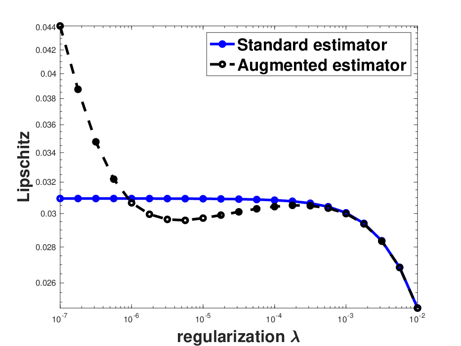
For both simulations, we use K=40K=40 in data augmentation. We repeat the simulation 100 times, and the average estimated MSE and Lipschitz constants of the standard estimator (5) and the augmented estimator (7) over a grid of regularization parameters are presented in Figure 1. It shows that the generalization error and the Lipschitz constant of augmented estimators decrease as λ\lambda increases from 00; and after an ‘optimal’ point in the order of ϵ2\epsilon^{2} it would increase. (We remark that the small Lipschitz constant for large λ\lambda is due to the fact that the f^\hat{f} converges to 00 and therefore its Lipschitz constant converges to 00.) This implies that without sufficient regularization, augmented estimators have overfitting problems and produce functions that are not robust, but both problems problem can be mitigated using regularization. In fact, augmented estimators with appropriate regularization perform better than the standard estimator, which performs better than augmented estimators with insufficient regularization. This verifies our theoretical investigation in Section 4. We also note that as a comparison, the standard regression does not suffer from overfitting.

Refer to caption
Refer to caption
Refer to caption
Refer to caption
Figure 1: The recorded Lip¯\overline{\mathrm{Lip}} and MSE¯\overline{{\mathrm{MSE}}} for augmented and standard estimators in simulated data sets for various choices of the regularization parameter. The first row represents setting 1, and the second row represents setting 2.
regularization 10−1410^{-14} 10−1310^{-13} 10−1210^{-12} 10−1110^{-11} 10−1010^{-10} 10−910^{-9} 10−810^{-8} 10−710^{-7}
(2,7)
MSE¯augment\overline{{\mathrm{MSE}}}_{\text{augment}} 0.1615 0.1614 0.1603 0.1610 0.1831 0.2080 0.2141 0.2148
MSE¯standard\overline{{\mathrm{MSE}}}_{\text{standard}} 0.2149 0.2149 0.2149 0.2149 0.2149 0.2149 0.2149 0.2149
Lip¯augment\overline{\mathrm{Lip}}_{\text{augment}} 3.3203 3.3198 3.3284 3.5998 4.6664 5.5526 5.7744 5.8003
Lip¯standard\overline{\mathrm{Lip}}_{\text{standard}} 5.8059 5.8059 5.8059 5.8059 5.8059 5.8058 5.8056 5.8035
(3,4)
MSE¯augment\overline{{\mathrm{MSE}}}_{\text{augment}} 0.0968 0.0967 0.0965 0.0993 0.1207 0.1432 0.1486 0.1493
MSE¯standard\overline{{\mathrm{MSE}}}_{\text{standard}} 0.1494 0.1494 0.1494 0.1494 0.1494 0.1494 0.1494 0.1493
Lip¯augment\overline{\mathrm{Lip}}_{\text{augment}} 3.1697 3.1699 3.1806 3.4031 4.2551 4.9986 5.1918 5.2144
Lip¯standard\overline{\mathrm{Lip}}_{\text{standard}} 5.2193 5.2193 5.2193 5.2193 5.2193 5.2192 5.2191 5.2172
(1,6)
MSE¯augment\overline{{\mathrm{MSE}}}_{\text{augment}} 0.0685 0.0680 0.0646 0.0607 0.0720 0.0852 0.0884 0.0887
MSE¯standard\overline{{\mathrm{MSE}}}_{\text{standard}} 0.0888 0.0888 0.0888 0.0888 0.0888 0.0888 0.0888 0.0888
Lip¯augment\overline{\mathrm{Lip}}_{\text{augment}} 3.6859 3.6601 3.5097 3.4695 4.2919 4.9662 5.1366 5.1533
Lip¯standard\overline{\mathrm{Lip}}_{\text{standard}} 5.1616 5.1616 5.1616 5.1616 5.1616 5.1616 5.1610 5.1558
Table 1: Experiments on MNIST data set for three pairs of digits: (2,7), (3,4), (1,6). The recorded Lip¯\overline{\mathrm{Lip}} and MSE¯\overline{{\mathrm{MSE}}} for augmented and standard estimators for various choices of the regularization parameter λ\lambda are shown, and the smallest MSE and Lipschitz constants are marked in bold.

Our second data set is sampled from MNIST [30]. For each pair of distinct digits (i,j)(i,j), where i,j∈{0,1,⋯,9},i,j\in\{0,1,\cdots,9\}, label one digit as 11 and the other as −1-1. For each simulation, the training set has 100100 samples and the testing set has 20002000 samples. We follow [32] and use the Gaussian kernel k(𝐱,𝐱′)=exp(−∥𝐱−𝐱′∥2/768)k(\mathbf{x},\mathbf{x}^{\prime})=\exp(-\|\mathbf{x}-\mathbf{x}^{\prime}\|^{2}/768) and K=40K=40 in data augmentation. We remark that the training samples are rather small to ensure that the augmented estimator can be computed as its size is KK times larger. The results are recorded in Table 1, in which a similar phenomenon as in Figure 1 have been observed: with small regularization parameters, the augmented estimators does not perform as well as the augmented estimators with appropriate regularizations. However, it is slightly different than Figure 1 and our findings in Section 4 in the sense that even with a very small λ\lambda, the augmented estimator f^λ(a​u​g)\hat{f}^{(aug)}_{\lambda} still outperforms the standard estimator f^0\hat{f}_{0}. We suspect that it might be due to numerical issues when some singular values of 𝐊𝐗\mathbf{K}_{\mathbf{X}} or 𝐓𝐗\mathbf{T}_{\mathbf{X}} are small.

Adversarial estimator We perform simulations on the adversarial estimator (6) separately as there is no explicit solution and the commonly used gradient descent algorithm [18] for adversarial training converges slowly. Instead, we record the MSE¯\overline{{\mathrm{MSE}}} and Lip¯\overline{\mathrm{Lip}} for the estimated functions over the iterations gradient descent, since early stopping in a ridgeless regression can be viewed as a form of regularization. For the simplicity of calculation, we apply a variant of (6), following the idea similar to (18):

f^λ(a​d​v)\displaystyle\hat{f}_{\lambda}^{(adv)} =argminf∈ℋ​1n​∑i=1nmaxδ∈𝚫i⁡(yi−f⁡(𝐱+δ))2+λ​‖f‖ℋ2,\displaystyle=\mbox{argmin}_{f\in{\cal H}}\frac{1}{n}\sum_{i=1}^{n}\max_{\mathbf{\delta}\in\mathbf{\Delta}_{i}}(y_{i}-f(\mathbf{x}+\mathbf{\delta}))^{2}+\lambda\|f\|_{{\cal H}}^{2}, (19)

where 𝚫i\mathbf{\Delta}_{i} is generated using the method after (18). Here we use the simulated data set of setting 1 and let the step size at the kk-th iteration be min⁡(0.04,4/k0.5)\min(0.04,4/k^{0.5}). The performance of adversarial training over iteration is recorded in Table 2 and we use the average over 50 repeats. It verifies the findings in Section 4 that adversarial training overfits in terms of both generalization error and Lipschitz constant, and regulatizations mitigates the overfitting issue.

iterations 1010 3030 100100 300300 10001000 30003000 1000010000 3000030000
MSE 0.2378 0.2353 0.1555 0.1422 0.1357 0.1377 0.1444 0.1511
Lipschitz 0.0462 0.0397 0.0294 0.0293 0.0285 0.0286 0.0323 0.0353
Table 2: The recorded Lip¯\overline{\mathrm{Lip}} and MSE¯\overline{{\mathrm{MSE}}} of ridgeless adversarial training over iterations on the simulated data set described in setting 1.

6 Conclusion

This paper presents a study of the performance of adversarial and augmented kernel regression compared to the ridgeless standard regression, and derives limiting formulas for these methods. The analysis reveals that when the regularization parameter is small, augmented or adversarial regression may lead to unstable performance, with worse generalization error and Lipschitz constant than ridgeless standard regression. However, with appropriate regularization, the regularized augmented or adversarial estimators outperform the ridgeless standard regression, demonstrating the effectiveness of regularization in adversarial training and data augmentation with noise, which differs from the standard kernel regression setting where overfitting is generally not a concern.

In future work, it would be interesting to explore the impact of ϵ\epsilon that does not depend on nn and 𝐗\mathbf{X}, which might be more realistic in settings with very large values of nn. Additionally, it would be valuable to investigate strategies for choosing an optimal value of λ\lambda or the best early stopping criterion based on the kernel and data sets.

7 Proof

Proof of Theorem 1.

(a) To prove Theorem 1, we first establish the following lemma:

Lemma 6 (Perturbation of a linear system).

(a) Assuming that 𝐀,𝐁∈ℝm×p,𝐲∈ℝm\mathbf{A},\mathbf{B}\in{\mathbb{R}}^{m\times p},\mathbf{y}\in{\mathbb{R}}^{m}, r​a​n​k​(𝐀)=n<mrank(\mathbf{A})=n<m, 𝐲∈Span​(𝐀)\mathbf{y}\in\mbox{Span}(\mathbf{A}), where Span​(𝐀)\mbox{Span}(\mathbf{A}) represents the column space of 𝐀\mathbf{A}, 𝐂=𝐀+ϵ​𝐁\mathbf{C}=\mathbf{A}+\epsilon\mathbf{B}, and let

𝐱~=argmin𝐱∈ℝp​‖𝐂𝐱−𝐲‖2+λ​‖𝐱‖2,𝐱^=argmin𝐱∈ℝp​‖𝐀𝐱−𝐲‖2+λ​‖𝐱‖2,\tilde{\mathbf{x}}=\mbox{argmin}_{\mathbf{x}\in{\mathbb{R}}^{p}}\|\mathbf{C}\mathbf{x}-\mathbf{y}\|^{2}+\lambda\|\mathbf{x}\|^{2},\hat{\mathbf{x}}=\mbox{argmin}_{\mathbf{x}\in{\mathbb{R}}^{p}}\|\mathbf{A}\mathbf{x}-\mathbf{y}\|^{2}+\lambda\|\mathbf{x}\|^{2},

then

‖𝐱~−𝐱^‖=O⁡(ϵ2/λ+ϵσn​(𝐀)).\|\tilde{\mathbf{x}}-\hat{\mathbf{x}}\|=O\Big(\frac{\epsilon^{2}/\lambda+\epsilon}{\sigma_{n}(\mathbf{A})}\Big).

(b) If in addition 𝐀𝐁T=0\mathbf{A}\mathbf{B}^{T}=0, σn​(𝐀)=O​(1)\sigma_{n}(\mathbf{A})=O(1), and let L∈ℝpL\in{\mathbb{R}}^{p} be the row space of 𝐀\mathbf{A}, then

‖𝐱~−𝐱^+(𝐏𝐋⟂T​𝐁𝐁T​𝐏𝐋⟂+λϵ2​𝐈)−1​𝐏𝐋⟂T​𝐁𝐁T​𝐏𝐋​𝐱^‖=O⁡(ϵ4/λ+ϵ2).\Big\|\tilde{\mathbf{x}}-\hat{\mathbf{x}}+\Big(\mathbf{P}_{\mathbf{L}^{\perp}}^{T}\mathbf{B}\mathbf{B}^{T}\mathbf{P}_{\mathbf{L}^{\perp}}+\frac{\lambda}{\epsilon^{2}}\mathbf{I}\Big)^{-1}\mathbf{P}_{\mathbf{L}^{\perp}}^{T}\mathbf{B}\mathbf{B}^{T}\mathbf{P}_{\mathbf{L}}\hat{\mathbf{x}}\Big\|=O(\epsilon^{4}/\lambda+\epsilon^{2}).

The proof of Theorem 1(a) is divided into two components. First, we will show that f~λ(a​u​g)\tilde{f}^{(aug)}_{\lambda} and f^λ(a​u​g)\hat{f}^{(aug)}_{\lambda} are close; second, f~λ(a​u​g)\tilde{f}^{(aug)}_{\lambda} and gλg_{\lambda} are close. Both components depend on Lemma 6.

For the first component, note that f^λ(a​u​g)\hat{f}^{(aug)}_{\lambda} and f~λ(a​u​g)\tilde{f}^{(aug)}_{\lambda} can be considered as linear systems with n×|𝚫|n\times|\mathbf{\Delta}| measure vectors (here |𝚫||\mathbf{\Delta}| can be infinity), represented by K𝐱i+δK_{\mathbf{x}_{i}+\mathbf{\delta}} and K𝐱i+𝐓𝐱i​𝚫K_{\mathbf{x}_{i}}+\mathbf{T}_{\mathbf{x}_{i}}\mathbf{\Delta} respectively. In addition, K𝐱i+δ−(K𝐱i+𝐓𝐱i​𝚫)=O⁡(ϵ2)K_{\mathbf{x}_{i}+\mathbf{\delta}}-(K_{\mathbf{x}_{i}}+\mathbf{T}_{\mathbf{x}_{i}}\mathbf{\Delta})=O(\epsilon^{2}). Then, Lemma 6(a) with 𝐀\mathbf{A} being a matrix with row vectors K𝐱i+𝐓𝐱i​𝚫K_{\mathbf{x}_{i}}+\mathbf{T}_{\mathbf{x}_{i}}\mathbf{\Delta}, 𝐂\mathbf{C} being a matrix with row vectors K𝐱i+δK_{\mathbf{x}_{i}+\mathbf{\delta}}, yiy_{i} being the corresponding measurement of K𝐱i+δK_{\mathbf{x}_{i}+\mathbf{\delta}}, ϵ\epsilon replaced with ϵ2\epsilon^{2}, nn replaced with n⁡(p+1)n(p+1). By the assumption, we have the n⁡(p+1)n(p+1)-th singular values of the matrix with row vectors K𝐱i+𝐓𝐱i​𝚫K_{\mathbf{x}_{i}}+\mathbf{T}_{\mathbf{x}_{i}}\mathbf{\Delta} is in the order of Ω⁡(ϵ)\Omega(\epsilon), and it can be verified that 𝐲∈Span​(𝐀)\mathbf{y}\in\mbox{Span}(\mathbf{A}) (note that by solving the system of K𝐱i​𝐳=yiK_{\mathbf{x}_{i}}\mathbf{z}=y_{i} and 𝐓𝐱i​𝐳=0\mathbf{T}_{\mathbf{x}_{i}}\mathbf{z}=0), so we have

‖f~λ(a​u​g)−f^λ+(𝐏𝐊𝐗⟂T​𝐁T​𝐁𝐏𝐊𝐗⟂+λϵ2​𝐈)−1​𝐏𝐊𝐗⟂T​𝐁T​𝐁𝐏𝐊𝐗​f^λ‖=O⁡(ϵ4/λ+ϵ2ϵ)=O⁡(ϵ3/λ+ϵ).\Big\|\tilde{f}^{(aug)}_{\lambda}-\hat{f}_{\lambda}+\Big(\mathbf{P}_{\mathbf{K}_{\mathbf{X}}^{\perp}}^{T}\mathbf{B}^{T}\mathbf{B}\mathbf{P}_{\mathbf{K}_{\mathbf{X}}^{\perp}}+\frac{\lambda}{\epsilon^{2}}\mathbf{I}\Big)^{-1}\mathbf{P}_{\mathbf{K}_{\mathbf{X}}^{\perp}}^{T}\mathbf{B}^{T}\mathbf{B}\mathbf{P}_{\mathbf{K}_{\mathbf{X}}}\hat{f}_{\lambda}\Big\|=O\Big(\frac{\epsilon^{4}/\lambda+\epsilon^{2}}{\epsilon}\Big)=O\Big(\epsilon^{3}/\lambda+\epsilon\Big). (20)

For the second part, applying Lemma 6(b) with 𝐀\mathbf{A} being a matrix with row vectors K𝐱iK_{\mathbf{x}_{i}} and 𝐂\mathbf{C} being a matrix with row vectors K𝐱i+𝐓𝐱i​𝚫K_{\mathbf{x}_{i}}+\mathbf{T}_{\mathbf{x}_{i}}\mathbf{\Delta}. Since Expect​𝚫=0\mathrm{Expect}\mathbf{\Delta}=0, we have 𝐀𝐁T=𝐀𝐂T−𝐀𝐀T=0\mathbf{A}\mathbf{B}^{T}=\mathbf{A}\mathbf{C}^{T}-\mathbf{A}\mathbf{A}^{T}=0. In addition, the rank of 𝐀\mathbf{A} is nn and σn​(𝐀)=Ω​(1)\sigma_{n}(\mathbf{A})=\Omega(1) by assumption, and 𝐂−𝐀=O⁡(ϵ)\mathbf{C}-\mathbf{A}=O(\epsilon), so Lemma 6(b) implies that

‖f~λ(a​u​g)−f^λ+(𝐏𝐋⟂T​𝚺​𝐏𝐋⟂+λϵ2​𝐈)−1​𝐏𝐋⟂T​𝚺​𝐏𝐋​f^λ‖=O⁡(ϵ4/λ+ϵ2).\Big\|\tilde{f}^{(aug)}_{\lambda}-\hat{f}_{\lambda}+\Big(\mathbf{P}_{\mathbf{L}^{\perp}}^{T}\mathbf{\Sigma}\mathbf{P}_{\mathbf{L}^{\perp}}+\frac{\lambda}{\epsilon^{2}}\mathbf{I}\Big)^{-1}\mathbf{P}_{\mathbf{L}^{\perp}}^{T}\mathbf{\Sigma}\mathbf{P}_{\mathbf{L}}\hat{f}_{\lambda}\Big\|=O(\epsilon^{4}/\lambda+\epsilon^{2}). (21)

Combining (20) and (21), (10) is proved.

(b) Note that

ℒ^(a​u​g)​(g0)=ℒ~(a​u​g)​(g0)+(ℒ^(a​u​g)​(g0)−ℒ~(a​u​g)​(g0))+λ​‖g0‖2=0+O⁡(ϵ4+λ)=O⁡(ϵ4+λ),\hat{{\mathcal{L}}}^{(aug)}(g_{0})=\tilde{{\mathcal{L}}}^{(aug)}(g_{0})+(\hat{{\mathcal{L}}}^{(aug)}(g_{0})-\tilde{{\mathcal{L}}}^{(aug)}(g_{0}))+\lambda\|g_{0}\|^{2}=0+O(\epsilon^{4}+\lambda)=O(\epsilon^{4}+\lambda),

and

ℒ^(a​u​g)​(f)≥C​ϵ2​‖PSpan​(𝐊𝐗,𝐓𝐗)​fλ−g0‖2,\hat{{\mathcal{L}}}^{(aug)}(f)\geq C\epsilon^{2}\Big\|P_{\mbox{Span}(\mathbf{K}_{\mathbf{X}},\mathbf{T}_{\mathbf{X}})}f_{\lambda}-g_{0}\Big\|^{2},

Theorem 1(b) is proved.

Proof of Lemma 6.

(a) Since 𝐲∈Span​(𝐀)\mathbf{y}\in\mbox{Span}(\mathbf{A}), WLOG we may rearrange the space ℝm{\mathbb{R}}^{m} and assume that

𝐀=(𝐀1𝟎(m−n)×p),𝐲=(𝐱1𝟎m−n),𝐁=(𝐁1𝐁2),\mathbf{A}=\begin{pmatrix}\mathbf{A}_{1}\\ \mathbf{0}_{(m-n)\times p}\end{pmatrix},\,\,\mathbf{y}=\begin{pmatrix}\mathbf{x}_{1}\\ \mathbf{0}_{m-n}\end{pmatrix},\,\,\,\mathbf{B}=\begin{pmatrix}\mathbf{B}_{1}\\ \mathbf{B}_{2}\end{pmatrix},

for some 𝐀1,𝐁1∈ℝn×p\mathbf{A}_{1},\mathbf{B}_{1}\in{\mathbb{R}}^{n\times p}, 𝐱1∈ℝn\mathbf{x}_{1}\in{\mathbb{R}}^{n}, and 𝐁2∈ℝm−n×p\mathbf{B}_{2}\in{\mathbb{R}}^{m-n\times p}.

Then we have

𝐱~=𝐂T​(𝐂𝐂T+λ​𝐈)−1​(𝐱1𝟎m−n)\displaystyle\tilde{\mathbf{x}}=\mathbf{C}^{T}(\mathbf{C}\mathbf{C}^{T}+\lambda\mathbf{I})^{-1}\begin{pmatrix}\mathbf{x}_{1}\\ \mathbf{0}_{m-n}\end{pmatrix}
=\displaystyle= (𝐀1+ϵ​𝐁1𝐁2)T​((𝐀1+ϵ​𝐁1)​(𝐀1+ϵ​𝐁1)T+λ​𝐈(𝐀1+ϵ​𝐁1)​ϵ​𝐁2Tϵ​𝐁2​(𝐀1+ϵ​𝐁1)Tϵ2​𝐁2​𝐁2T+λ​𝐈)−1​(𝐱1𝟎m−n)\displaystyle\begin{pmatrix}\mathbf{A}_{1}+\epsilon\mathbf{B}_{1}\\ \mathbf{B}_{2}\end{pmatrix}^{T}\begin{pmatrix}(\mathbf{A}_{1}+\epsilon\mathbf{B}_{1})(\mathbf{A}_{1}+\epsilon\mathbf{B}_{1})^{T}+\lambda\mathbf{I}&(\mathbf{A}_{1}+\epsilon\mathbf{B}_{1})\epsilon\mathbf{B}_{2}^{T}\\ \epsilon\mathbf{B}_{2}(\mathbf{A}_{1}+\epsilon\mathbf{B}_{1})^{T}&\epsilon^{2}\mathbf{B}_{2}\mathbf{B}_{2}^{T}+\lambda\mathbf{I}\end{pmatrix}^{-1}\begin{pmatrix}\mathbf{x}_{1}\\ \mathbf{0}_{m-n}\end{pmatrix}
=\displaystyle= (𝐀1+ϵ​𝐁1𝐁2)T​(𝐙∗−(ϵ2​𝐁2​𝐁2T+λ​𝐈)−1​(ϵ​𝐁2​(𝐀1+ϵ​𝐁1)T)​𝐙∗)​(𝐱10)\displaystyle\begin{pmatrix}\mathbf{A}_{1}+\epsilon\mathbf{B}_{1}\\ \mathbf{B}_{2}\end{pmatrix}^{T}\begin{pmatrix}\mathbf{Z}&*\\ -(\epsilon^{2}\mathbf{B}_{2}\mathbf{B}_{2}^{T}+\lambda\mathbf{I})^{-1}(\epsilon\mathbf{B}_{2}(\mathbf{A}_{1}+\epsilon\mathbf{B}_{1})^{T})\mathbf{Z}&*\end{pmatrix}\begin{pmatrix}\mathbf{x}_{1}\\ 0\end{pmatrix}
=\displaystyle= (𝐈−ϵ​𝐁2T​(ϵ2​𝐁2​𝐁2T+λ​𝐈)−1​ϵ​𝐁2)​(𝐀1+ϵ​𝐁1)T​𝐙𝐱1.\displaystyle\Big(\mathbf{I}-\epsilon\mathbf{B}_{2}^{T}(\epsilon^{2}\mathbf{B}_{2}\mathbf{B}_{2}^{T}+\lambda\mathbf{I})^{-1}\epsilon\mathbf{B}_{2}\Big)(\mathbf{A}_{1}+\epsilon\mathbf{B}_{1})^{T}\mathbf{Z}\mathbf{x}_{1}. (22)

where the expression of 𝐙\mathbf{Z} follows from the well-known 2×22\times 2 block matrix inversion formula

(𝐀𝐔𝐕𝐂)−1=((𝐀−𝐔𝐂−1​𝐕)−1−(𝐀−𝐔𝐂−1​𝐕)−1​𝐔𝐂−1−𝐂−1​𝐕​(𝐀−𝐔𝐂−1​𝐕)−1𝐂−1+𝐂−1​𝐕​(𝐀−𝐔𝐂−1​𝐕)−1​𝐔𝐂−1)\begin{pmatrix}\mathbf{A}&\mathbf{U}\\ \mathbf{V}&\mathbf{C}\end{pmatrix}^{-1}=\begin{pmatrix}(\mathbf{A}-\mathbf{U}\mathbf{C}^{-1}\mathbf{V})^{-1}&-(\mathbf{A}-\mathbf{U}\mathbf{C}^{-1}\mathbf{V})^{-1}\mathbf{U}\mathbf{C}^{-1}\\ -\mathbf{C}^{-1}\mathbf{V}(\mathbf{A}-\mathbf{U}\mathbf{C}^{-1}\mathbf{V})^{-1}&\mathbf{C}^{-1}+\mathbf{C}^{-1}\mathbf{V}(\mathbf{A}-\mathbf{U}\mathbf{C}^{-1}\mathbf{V})^{-1}\mathbf{U}\mathbf{C}^{-1}\end{pmatrix} (23)

and we have

𝐙−1=\displaystyle\mathbf{Z}^{-1}= (𝐀1+ϵ​𝐁1)​(𝐀1+ϵ​𝐁1)T+λ​𝐈−(𝐀1+ϵ​𝐁1)​ϵ​𝐁2T​(ϵ2​𝐁2​𝐁2T+λ​𝐈)−1​ϵ​𝐁2​(𝐀1+ϵ​𝐁1)T\displaystyle(\mathbf{A}_{1}+\epsilon\mathbf{B}_{1})(\mathbf{A}_{1}+\epsilon\mathbf{B}_{1})^{T}+\lambda\mathbf{I}-(\mathbf{A}_{1}+\epsilon\mathbf{B}_{1})\epsilon\mathbf{B}_{2}^{T}(\epsilon^{2}\mathbf{B}_{2}\mathbf{B}_{2}^{T}+\lambda\mathbf{I})^{-1}\epsilon\mathbf{B}_{2}(\mathbf{A}_{1}+\epsilon\mathbf{B}_{1})^{T}
=\displaystyle= (𝐀1+ϵ​𝐁1)​𝐐​(𝐀1+ϵ​𝐁1)T+λ​𝐈\displaystyle(\mathbf{A}_{1}+\epsilon\mathbf{B}_{1})\mathbf{Q}(\mathbf{A}_{1}+\epsilon\mathbf{B}_{1})^{T}+\lambda\mathbf{I}

for the symmetric matrix 𝐐=𝐈−ϵ​𝐁2T​(ϵ2​𝐁2​𝐁2T+λ​𝐈)−1​ϵ​𝐁2=𝐈+O⁡(ϵ2/λ)\mathbf{Q}=\mathbf{I}-\epsilon\mathbf{B}_{2}^{T}(\epsilon^{2}\mathbf{B}_{2}\mathbf{B}_{2}^{T}+\lambda\mathbf{I})^{-1}\epsilon\mathbf{B}_{2}=\mathbf{I}+O(\epsilon^{2}/\lambda). Then

(𝐀1+ϵ𝐁1)T𝐙=(𝐀1+ϵ𝐁1)T((𝐀1+ϵ𝐁1)𝐐(𝐀1+ϵ𝐁1)T+λ𝐈)−1=𝐐−1/2f(𝐐1/2(𝐀1+ϵ𝐁1))(\mathbf{A}_{1}+\epsilon\mathbf{B}_{1})^{T}\mathbf{Z}=(\mathbf{A}_{1}+\epsilon\mathbf{B}_{1})^{T}\Big((\mathbf{A}_{1}+\epsilon\mathbf{B}_{1})\mathbf{Q}(\mathbf{A}_{1}+\epsilon\mathbf{B}_{1})^{T}+\lambda\mathbf{I}\Big)^{-1}=\mathbf{Q}^{-1/2}f(\mathbf{Q}^{1/2}(\mathbf{A}_{1}+\epsilon\mathbf{B}_{1})) (24)

for f⁡(𝐗)=𝐗T​(𝐗𝐗T+λ​𝐈)−1.f(\mathbf{X})=\mathbf{X}^{T}(\mathbf{X}\mathbf{X}^{T}+\lambda\mathbf{I})^{-1}. Since f⁡(𝐗)f(\mathbf{X}) is continuous at 𝐗\mathbf{X} with locally Lipschitz constant 1/σmin​(𝐗)1/\sigma_{\min}(\mathbf{X}) (add citations) and 𝐐1/2​(𝐀1+ϵ​𝐁1)−𝐀1=O⁡(ϵ2/λ+ϵ)\mathbf{Q}^{1/2}(\mathbf{A}_{1}+\epsilon\mathbf{B}_{1})-\mathbf{A}_{1}=O(\epsilon^{2}/\lambda+\epsilon), (24) implies that if ϵ​‖𝐁1‖<σmin​(𝐀)/2\epsilon\|\mathbf{B}_{1}\|<\sigma_{\min}(\mathbf{A})/2, then

(𝐀1+ϵ​𝐁1)T​𝐙=f⁡(𝐀1)+O⁡(ϵ2/λ+ϵσmin​(𝐀1))=𝐀1T​(𝐀1​𝐀1T+λ​𝐈)−1+O⁡(ϵ2/λ+ϵσmin​(𝐀1)).(\mathbf{A}_{1}+\epsilon\mathbf{B}_{1})^{T}\mathbf{Z}=f(\mathbf{A}_{1})+O\Big(\frac{\epsilon^{2}/\lambda+\epsilon}{\sigma_{\min}(\mathbf{A}_{1})}\Big)=\mathbf{A}_{1}^{T}(\mathbf{A}_{1}\mathbf{A}_{1}^{T}+\lambda\mathbf{I})^{-1}+O\Big(\frac{\epsilon^{2}/\lambda+\epsilon}{\sigma_{\min}(\mathbf{A}_{1})}\Big). (25)

Combining (22) and (25) and ϵ​𝐁2T​(ϵ2​𝐁2​𝐁2T+λ​𝐈)−1​ϵ​𝐁2=O⁡(ϵ2/λ)\epsilon\mathbf{B}_{2}^{T}(\epsilon^{2}\mathbf{B}_{2}\mathbf{B}_{2}^{T}+\lambda\mathbf{I})^{-1}\epsilon\mathbf{B}_{2}=O(\epsilon^{2}/\lambda), 𝐱^=𝐀T​(𝐀𝐀T+λ​𝐈)−1​𝐲=𝐀1T​(𝐀1​𝐀1T+λ​𝐈)−1​𝐱1\hat{\mathbf{x}}=\mathbf{A}^{T}(\mathbf{A}\mathbf{A}^{T}+\lambda\mathbf{I})^{-1}\mathbf{y}=\mathbf{A}_{1}^{T}(\mathbf{A}_{1}\mathbf{A}_{1}^{T}+\lambda\mathbf{I})^{-1}\mathbf{x}_{1}, as well as σmin​(𝐀)=σmin​(𝐀1){\sigma_{\min}(\mathbf{A})}={\sigma_{\min}(\mathbf{A}_{1})} we have that if ϵ​‖𝐁‖<σmin​(𝐀)/2\epsilon\|\mathbf{B}\|<\sigma_{\min}(\mathbf{A})/2, then

‖𝐱~−𝐱^‖=O⁡(ϵ2/λ+ϵσmin​(𝐀)).\|\tilde{\mathbf{x}}-\hat{\mathbf{x}}\|=O\Big(\frac{\epsilon^{2}/\lambda+\epsilon}{\sigma_{\min}(\mathbf{A})}\Big).

(b) If the column spaces of 𝐀\mathbf{A} and 𝐁\mathbf{B} are perpendicular, then we may rearrange the row space in ℝp{\mathbb{R}}^{p} such that

𝐀=(𝐀11,00,0),𝐁=(0,0𝐁21,𝐁22)\mathbf{A}=\begin{pmatrix}\mathbf{A}_{11},0\\ 0,0\end{pmatrix},\,\,\,\mathbf{B}=\begin{pmatrix}0,0\\ \mathbf{B}_{21},\mathbf{B}_{22}\end{pmatrix}

for 𝐀11∈ℝn×n\mathbf{A}_{11}\in{\mathbb{R}}^{n\times n}, 𝐁21∈ℝ(m−n)×n\mathbf{B}_{21}\in{\mathbb{R}}^{(m-n)\times n}, and 𝐁22∈ℝ(m−n)×(p−n)\mathbf{B}_{22}\in{\mathbb{R}}^{(m-n)\times(p-n)}. Note that there is a connection that 𝐀1=(𝐀11,0),𝐁1=0,𝐁2=(𝐁21,𝐁22).\mathbf{A}_{1}=\begin{pmatrix}\mathbf{A}_{11},0\end{pmatrix},\mathbf{B}_{1}=0,\mathbf{B}_{2}=\begin{pmatrix}\mathbf{B}_{21},\mathbf{B}_{22}\end{pmatrix}.

Then we have 𝐂T​𝐂=𝐀T​𝐀+ϵ2​𝐁T​𝐁\mathbf{C}^{T}\mathbf{C}=\mathbf{A}^{T}\mathbf{A}+\epsilon^{2}\mathbf{B}^{T}\mathbf{B}, and

𝐱^=(𝐂T​𝐂+λ​𝐈)−1​𝐂T​(𝐱1𝟎)\displaystyle\hat{\mathbf{x}}=(\mathbf{C}^{T}\mathbf{C}+\lambda\mathbf{I})^{-1}\mathbf{C}^{T}\begin{pmatrix}\mathbf{x}_{1}\\ \mathbf{0}\end{pmatrix}
=\displaystyle= (𝐀11T​𝐀11+ϵ2​𝐁21T​𝐁21+λ​𝐈ϵ2​𝐁21T​𝐁22ϵ2​𝐁22T​𝐁21ϵ2​𝐁22T​𝐁22+λ​𝐈)−1​(𝐀11​𝐱10)\displaystyle\begin{pmatrix}\mathbf{A}_{11}^{T}\mathbf{A}_{11}+\epsilon^{2}\mathbf{B}_{21}^{T}\mathbf{B}_{21}+\lambda\mathbf{I}&\epsilon^{2}\mathbf{B}_{21}^{T}\mathbf{B}_{22}\\ \epsilon^{2}\mathbf{B}_{22}^{T}\mathbf{B}_{21}&\epsilon^{2}\mathbf{B}_{22}^{T}\mathbf{B}_{22}+\lambda\mathbf{I}\end{pmatrix}^{-1}\begin{pmatrix}\mathbf{A}_{11}\mathbf{x}_{1}\\ 0\end{pmatrix}
=\displaystyle= (𝐙∗−(ϵ2​𝐁22T​𝐁22+λ​𝐈)−1​ϵ2​𝐁22T​𝐁21​𝐙∗)​(𝐀11​𝐱10)\displaystyle\begin{pmatrix}\mathbf{Z}&*\\ -(\epsilon^{2}\mathbf{B}_{22}^{T}\mathbf{B}_{22}+\lambda\mathbf{I})^{-1}\epsilon^{2}\mathbf{B}_{22}^{T}\mathbf{B}_{21}\mathbf{Z}&*\end{pmatrix}\begin{pmatrix}\mathbf{A}_{11}\mathbf{x}_{1}\\ 0\end{pmatrix}

where

𝐙=\displaystyle\mathbf{Z}= (𝐀11T​𝐀11+ϵ2​𝐁21T​𝐁21+λ​𝐈−ϵ2​𝐁21T​𝐁22​(ϵ2​𝐁22T​𝐁22+λ​𝐈)−1​ϵ2​𝐁22T​𝐁21)−1\displaystyle\Big(\mathbf{A}_{11}^{T}\mathbf{A}_{11}+\epsilon^{2}\mathbf{B}_{21}^{T}\mathbf{B}_{21}+\lambda\mathbf{I}-\epsilon^{2}\mathbf{B}_{21}^{T}\mathbf{B}_{22}(\epsilon^{2}\mathbf{B}_{22}^{T}\mathbf{B}_{22}+\lambda\mathbf{I})^{-1}\epsilon^{2}\mathbf{B}_{22}^{T}\mathbf{B}_{21}\Big)^{-1}
=\displaystyle= (𝐀1​𝐀1T+λ​𝐈)−1+O⁡(ϵ4/λ+ϵ2)\displaystyle(\mathbf{A}_{1}\mathbf{A}_{1}^{T}+\lambda\mathbf{I})^{-1}+O(\epsilon^{4}/\lambda+\epsilon^{2})

follows from the inversion formula (23) and the fact that the minimum singular value of 𝐀11\mathbf{A}_{11} is O⁡(1)O(1). Note that here we applies the assumption that

‖ϵ2​𝐁21T​𝐁21+ϵ4​𝐁21T​𝐁22​𝐁22T​𝐁21/λ‖≤σmin​(𝐀1​𝐀1T)/2.\Big\|\epsilon^{2}\mathbf{B}_{21}^{T}\mathbf{B}_{21}+\epsilon^{4}\mathbf{B}_{21}^{T}\mathbf{B}_{22}\mathbf{B}_{22}^{T}\mathbf{B}_{21}/\lambda\Big\|\leq\sigma_{\min}(\mathbf{A}_{1}\mathbf{A}_{1}^{T})/2.

Part (b) then follows from 𝐙𝐀11​𝐱1=𝐱^+O⁡(ϵ4/λ+ϵ2)\mathbf{Z}\mathbf{A}_{11}\mathbf{x}_{1}=\hat{\mathbf{x}}+O(\epsilon^{4}/\lambda+\epsilon^{2}) and (ϵ2​𝐁22T​𝐁22+λ​𝐈)−1​ϵ2​𝐁22T​𝐁21​𝐙=(𝐏𝐋⟂T​𝐁T​𝐁𝐏𝐋⟂+λϵ2​𝐈)−1​𝐏𝐋⟂T​𝐁T​𝐁𝐏𝐋​𝐱^+O⁡(ϵ4/λ+ϵ2).(\epsilon^{2}\mathbf{B}_{22}^{T}\mathbf{B}_{22}+\lambda\mathbf{I})^{-1}\epsilon^{2}\mathbf{B}_{22}^{T}\mathbf{B}_{21}\mathbf{Z}=\Big(\mathbf{P}_{\mathbf{L}^{\perp}}^{T}\mathbf{B}^{T}\mathbf{B}\mathbf{P}_{\mathbf{L}^{\perp}}+\frac{\lambda}{\epsilon^{2}}\mathbf{I}\Big)^{-1}\mathbf{P}_{\mathbf{L}^{\perp}}^{T}\mathbf{B}^{T}\mathbf{B}\mathbf{P}_{\mathbf{L}}\hat{\mathbf{x}}+O(\epsilon^{4}/\lambda+\epsilon^{2}).

Proof of Theorem 2(a).

First, we summarize our findings in the following statement on the equivalence between f~λ(a​d​v)\tilde{f}^{(adv)}_{\lambda} and gλ′=f^0+(𝐏𝐊𝐗⟂T​𝚺​𝐏𝐊𝐗⟂+λϵ2​𝐈)−1​𝐏𝐊𝐗⟂T​𝚺​𝐏𝐊𝐗​f^0g_{\lambda}^{\prime}=\hat{f}_{0}+\Big(\mathbf{P}_{\mathbf{K}_{\mathbf{X}}^{\perp}}^{T}\mathbf{\Sigma}\mathbf{P}_{\mathbf{K}_{\mathbf{X}}^{\perp}}+\frac{\lambda}{\epsilon^{2}}\mathbf{I}\Big)^{-1}\mathbf{P}_{\mathbf{K}_{\mathbf{X}}^{\perp}}^{T}\mathbf{\Sigma}\mathbf{P}_{\mathbf{K}_{\mathbf{X}}}\hat{f}_{0}:

When λ=o⁡(ϵ)\lambda=o(\epsilon), f~λ(a​d​v)=gλ′\tilde{f}^{(adv)}_{\lambda}=g_{\lambda}^{\prime}. (26)

To prove (26), we only need to show that the derivative of ℒ~λ(a​d​v)\tilde{{\mathcal{L}}}^{(adv)}_{\lambda} at gλ′g_{\lambda}^{\prime} is zero. It is straightforward to verify that the objective function in (13) is equivalent to the expression

ℒ~λ(a​d​v)​(f)=1n​∑i=1n(|yi−⟨f,K𝐱i⟩|+ϵ​‖fT​𝐓𝐱i‖)2+λ​‖f‖ℋ2,\displaystyle\tilde{{\mathcal{L}}}^{(adv)}_{\lambda}(f)=\frac{1}{n}\sum_{i=1}^{n}\Big(|y_{i}-\langle f,K_{\mathbf{x}_{i}}\rangle|+\epsilon\|f^{T}\mathbf{T}_{\mathbf{x}_{i}}\|\Big)^{2}+\lambda\|f\|_{{\cal H}}^{2}, (27)

and we will evaluate the directional derivative at direction hh for both h∈Span​(𝐊𝐗)⟂h\in\mbox{Span}(\mathbf{K}_{\mathbf{X}})^{\perp} and h∈Span​(𝐊𝐗)h\in\mbox{Span}(\mathbf{K}_{\mathbf{X}}).

For h∈Span​(𝐊𝐗)⟂h\in\mbox{Span}(\mathbf{K}_{\mathbf{X}})^{\perp}, we have |yi−⟨f,K𝐱i+𝐓𝐱i​δ⟩|=0|y_{i}-\langle f,K_{\mathbf{x}_{i}}+\mathbf{T}_{\mathbf{x}_{i}}\mathbf{\delta}\rangle|=0 and ℒ~λ(a​d​v)=ϵ2n​∑i=1n‖fT​𝐓𝐱i‖2+λ​‖f‖ℋ2​(f)\tilde{{\mathcal{L}}}^{(adv)}_{\lambda}=\frac{\epsilon^{2}}{n}\sum_{i=1}^{n}\|f^{T}\mathbf{T}_{\mathbf{x}_{i}}\|^{2}+\lambda\|f\|_{{\cal H}}^{2}(f) for f∈Span​(gλ′,h)f\in\mbox{Span}(g_{\lambda}^{\prime},h). Then by the definition of (8), we have that the directional derivative at gλ′g_{\lambda}^{\prime} and direction hh is zero.

For h∈Span​(𝐊𝐗)h\in\mbox{Span}(\mathbf{K}_{\mathbf{X}}), the directional derivative of ℒ~(a​d​v)\tilde{{\mathcal{L}}}^{(adv)} at gλg_{\lambda} and direction hh is given by

2n​∑i=1n(ϵ​|gT​𝐓𝐱i|)​(|hT​K𝐱i|+ϵ​hT​𝐓𝐱i​𝐓𝐱iT​g|gT​𝐓𝐱i|)+2​λ​gT​h,\frac{2}{n}\sum_{i=1}^{n}\Big(\epsilon|g^{T}\mathbf{T}_{\mathbf{x}_{i}}|\Big)\Big(|h^{T}K_{\mathbf{x}_{i}}|+\epsilon\frac{h^{T}\mathbf{T}_{\mathbf{x}_{i}}\mathbf{T}_{\mathbf{x}_{i}}^{T}g}{|g^{T}\mathbf{T}_{\mathbf{x}_{i}}|}\Big)+2\lambda g^{T}h,

which is positive if

2n​∑i=1n|gT​𝐓𝐱i|​|hT​K𝐱i|≥2n​∑i=1nϵ​hT​𝐓𝐱i​𝐓𝐱iT​g+2​λϵ​gT​h.\frac{2}{n}\sum_{i=1}^{n}|g^{T}\mathbf{T}_{\mathbf{x}_{i}}||h^{T}K_{\mathbf{x}_{i}}|\geq\frac{2}{n}\sum_{i=1}^{n}\epsilon h^{T}\mathbf{T}_{\mathbf{x}_{i}}\mathbf{T}_{\mathbf{x}_{i}}^{T}g+2\frac{\lambda}{\epsilon}g^{T}h.

Considering that its LHS is in the order of O⁡(1)O(1), this is true if g=gλ′g=g_{\lambda}^{\prime} and λ=o⁡(ϵ)\lambda=o(\epsilon). As the derivative of ℒ~λ(a​d​v)\tilde{{\mathcal{L}}}^{(adv)}_{\lambda} at gλ′g_{\lambda}^{\prime} is zero, and ℒ~λ(a​d​v)\tilde{{\mathcal{L}}}^{(adv)}_{\lambda} is convex, (26) is proved.

Second, we will prove that f~λ(a​d​v)\tilde{f}^{(adv)}_{\lambda} and f^λ(a​d​v)\hat{f}^{(adv)}_{\lambda} are close. In the following we will simplify the notations and write gg instead of gλ′g_{\lambda}^{\prime}.The proof will be based on the expressions

∇ℒ^(a​d​v)λ(g)=−2n∑i=1n(yi−g(𝐱i+δi(g)))K𝐱i+δi​(g)+2λg,\displaystyle\text{$\nabla\hat{{\mathcal{L}}}^{(adv)}_{\lambda}(g)=-\frac{2}{n}\sum_{i=1}^{n}\Big(y_{i}-g\big(\mathbf{x}_{i}+\mathbf{\delta}_{i}(g)\big)\Big)K_{\mathbf{x}_{i}+\mathbf{\delta}_{i}(g)}+2\lambda g$}, (28)
∇ℒ~λ(a​d​v)(g)=−2n∑i=1n(yi−⟨g,K𝐱i+𝐓𝐱i𝚫i′(g)⟩)K𝐱i𝚫i′(g)+2λg\displaystyle\nabla\tilde{{\mathcal{L}}}^{(adv)}_{\lambda}(g)=-\frac{2}{n}\sum_{i=1}^{n}(y_{i}-\langle g,K_{\mathbf{x}_{i}}+\mathbf{T}_{\mathbf{x}_{i}}\mathbf{\Delta}_{i}^{\prime}(g)\rangle)K_{\mathbf{x}_{i}}\mathbf{\Delta}_{i}^{\prime}(g)+2\lambda g (29)

where δi(f)=argmaxδ:‖δ‖≤ϵ|yi−f(𝐱i+δ)|\mathbf{\delta}_{i}(f)=\arg\max_{\mathbf{\delta}:\|\mathbf{\delta}\|\leq\epsilon}|y_{i}-f(\mathbf{x}_{i}+\mathbf{\delta})|, and 𝚫i′(f)=argmaxδ:‖δ‖≤ϵ|yi−⟨f,K𝐱i+𝐓𝐱iδ⟩)|\mathbf{\Delta}_{i}^{\prime}(f)=\arg\max_{\mathbf{\delta}:\|\mathbf{\delta}\|\leq\epsilon}|y_{i}-\langle f,K_{\mathbf{x}_{i}}+\mathbf{T}_{\mathbf{x}_{i}}\mathbf{\delta}\rangle)|.

The proofs of (28) and (29) are similar. Note that for

ℒ⁡(f,{𝚫i}i=1n)=1n​∑i=1n(yi−f⁡(𝐱+δi))2+λ​‖f‖ℋ2,\mathcal{L}(f,\{\mathbf{\Delta}_{i}\}_{i=1}^{n})=\frac{1}{n}\sum_{i=1}^{n}(y_{i}-f(\mathbf{x}+\mathbf{\delta}_{i}))^{2}+\lambda\|f\|_{{\cal H}}^{2},

we have ∇𝚫ℒ​(g,{𝚫i​(g)}i=1n)=0\nabla_{\mathbf{\Delta}}\mathcal{L}(g,\{\mathbf{\Delta}_{i}(g)\}_{i=1}^{n})=0; and by continuity we have ∇𝚫ℒ​(g+h,{𝚫i​(g)}i=1n)=O⁡(‖h‖)\nabla_{\mathbf{\Delta}}\mathcal{L}(g+h,\{\mathbf{\Delta}_{i}(g)\}_{i=1}^{n})=O(\|h\|). Since ‖𝚫i​(g+h)−𝚫i​(g)‖=O⁡(h)\|\mathbf{\Delta}_{i}(g+h)-\mathbf{\Delta}_{i}(g)\|=O(h), we have

ℒ⁡(g+h,{𝚫i​(g+h)}i=1n)−ℒ⁡(g+h,{𝚫i​(g)}i=1n)=O⁡(‖h‖2).\mathcal{L}(g+h,\{\mathbf{\Delta}_{i}(g+h)\}_{i=1}^{n})-\mathcal{L}(g+h,\{\mathbf{\Delta}_{i}(g)\}_{i=1}^{n})=O(\|h\|^{2}).

So the directional derivative of ℒ^λ(a​d​v)\hat{{\mathcal{L}}}_{\lambda}^{(adv)} at gg with direction hh is given by

limt→0ℒ~λ(a​d​v)​(g+t​h)−ℒ~λ(a​d​v)​(g)t\displaystyle\lim_{t\rightarrow 0}\frac{\tilde{{\mathcal{L}}}^{(adv)}_{\lambda}(g+th)-\tilde{{\mathcal{L}}}^{(adv)}_{\lambda}(g)}{t}
=\displaystyle= limt→0ℒ⁡(g+t​h,{𝚫i​(g+t​h)}i=1n)−ℒ⁡(g+t​h,{𝚫i​(g+t​h)}i=1n)t\displaystyle\lim_{t\rightarrow 0}\frac{\mathcal{L}(g+th,\{\mathbf{\Delta}_{i}(g+th)\}_{i=1}^{n})-\mathcal{L}(g+th,\{\mathbf{\Delta}_{i}(g+th)\}_{i=1}^{n})}{t}
=\displaystyle= limt→0ℒ⁡(g+t​h,{𝚫i​(g+t​h)}i=1n)−ℒ⁡(g+t​h,{𝚫i​(g)}i=1n)t,\displaystyle\lim_{t\rightarrow 0}\frac{\mathcal{L}(g+th,\{\mathbf{\Delta}_{i}(g+th)\}_{i=1}^{n})-\mathcal{L}(g+th,\{\mathbf{\Delta}_{i}(g)\}_{i=1}^{n})}{t},

which then verifies (28). The proof of (29) is similar.

By definition, we have ‖g‖≤O⁡(1)\|g\|\leq O(1) and

maxδ:‖δ‖≤ϵ(yi−⟨g,K𝐱i+𝐓𝐱iδ⟩)2=⟨g,𝐓𝐱iδi′(g)⟩2≤∥g∥2∥𝐓𝐱i∥2∥δi′(g)∥2=O(ϵ2).\max_{\mathbf{\delta}:\|\mathbf{\delta}\|\leq\epsilon}(y_{i}-\langle g,K_{\mathbf{x}_{i}}+\mathbf{T}_{\mathbf{x}_{i}}\mathbf{\delta}\rangle)^{2}=\langle g,\mathbf{T}_{\mathbf{x}_{i}}\mathbf{\delta}_{i}^{\prime}(g)\rangle^{2}\leq\|g\|^{2}\|\mathbf{T}_{\mathbf{x}_{i}}\|^{2}\|\mathbf{\delta}_{i}^{\prime}(g)\|^{2}=O(\epsilon^{2}). (30)

In addition, we have

δi​(g)−δi′​(g)=O⁡(ϵ1.5),\displaystyle\mathbf{\delta}_{i}(g)-\mathbf{\delta}_{i}^{\prime}(g)=O(\epsilon^{1.5}), (31)

which can be proved as follows. WLOG assuming that ⟨g,𝐓𝐱i​δi′​(g)⟩>0\langle g,\mathbf{T}_{\mathbf{x}_{i}}\mathbf{\delta}_{i}^{\prime}(g)\rangle>0 and when ⟨g,𝐓𝐱i⟩=O⁡(1)\langle g,\mathbf{T}_{\mathbf{x}_{i}}\rangle=O(1), then for all δ∈B⁡(0,ϵ)∖B⁡(δi′​(g),ϵ1.5)\mathbf{\delta}\in B(0,\epsilon)\setminus B(\mathbf{\delta}_{i}^{\prime}(g),\epsilon^{1.5}), we have

⟨g,𝐓𝐱i​(δi′​(g)−δ)⟩>C​ϵ2.\langle g,\mathbf{T}_{\mathbf{x}_{i}}(\mathbf{\delta}_{i}^{\prime}(g)-\mathbf{\delta})\rangle>C\epsilon^{2}.

So δi​(g)≠δ\mathbf{\delta}_{i}(g)\neq\mathbf{\delta} as ⟨g,K𝐱+δ⟩≤⟨g,K𝐱i+δi′​(g)⟩\langle g,K_{\mathbf{x}+\mathbf{\delta}}\rangle\leq\langle g,K_{\mathbf{x}_{i}+\mathbf{\delta}_{i}^{\prime}(g)}\rangle.

We also have

(yi−⟨g,K𝐱i+δi​(g)⟩)−(yi−⟨g,K𝐱i+𝐓𝐱i​δi′​(g)⟩)=O⁡(ϵ2).(y_{i}-\langle g,K_{\mathbf{x}_{i}+\mathbf{\delta}_{i}(g)}\rangle)-(y_{i}-\langle g,K_{\mathbf{x}_{i}}+\mathbf{T}_{\mathbf{x}_{i}}\mathbf{\delta}_{i}^{\prime}(g)\rangle)=O(\epsilon^{2}). (32)

and the proof follows from the definition: if (yi−⟨g,K𝐱i+δi​(g)⟩)−(yi−⟨g,K𝐱i+𝐓𝐱i​δi′​(g)⟩)>C​ϵ2(y_{i}-\langle g,K_{\mathbf{x}_{i}+\mathbf{\delta}_{i}(g)}\rangle)-(y_{i}-\langle g,K_{\mathbf{x}_{i}}+\mathbf{T}_{\mathbf{x}_{i}}\mathbf{\delta}_{i}^{\prime}(g)\rangle)>C\epsilon^{2}, then (yi−⟨g,𝐓𝐱i​δi​(g)⟩)>(yi−⟨g,K𝐱i+𝐓𝐱i​δi′​(g)⟩)(y_{i}-\langle g,\mathbf{T}_{\mathbf{x}_{i}}\mathbf{\delta}_{i}(g)\rangle)>(y_{i}-\langle g,K_{\mathbf{x}_{i}}+\mathbf{T}_{\mathbf{x}_{i}}\mathbf{\delta}_{i}^{\prime}(g)\rangle), which is a contradiction to the definition of δi′​(g)\mathbf{\delta}_{i}^{\prime}(g). Similarly we do not have (yi−⟨g,K𝐱i+δi​(g)⟩)−(yi−⟨g,K𝐱i+𝐓𝐱i​δi′​(g)⟩)<−C​ϵ2(y_{i}-\langle g,K_{\mathbf{x}_{i}+\mathbf{\delta}_{i}(g)}\rangle)-(y_{i}-\langle g,K_{\mathbf{x}_{i}}+\mathbf{T}_{\mathbf{x}_{i}}\mathbf{\delta}_{i}^{\prime}(g)\rangle)<-C\epsilon^{2}, and (32) is proved.

Combining (28)-(29) with ∇ℒ~λ(a​d​v)​(g)=0\nabla\tilde{{\mathcal{L}}}_{\lambda}^{(adv)}(g)=0, we have

−∇ℒ^λ(a​d​v)​(g)=\displaystyle-\nabla\hat{{\mathcal{L}}}_{\lambda}^{(adv)}(g)= 2n​∑i=1n[(yi−⟨g,K𝐱i+δi​(g)⟩)−(yi−⟨g,K𝐱i+𝐓𝐱i​δi′​(g)⟩)]​K𝐱i+δi​(g)\displaystyle\frac{2}{n}\sum_{i=1}^{n}\Big[(y_{i}-\langle g,K_{\mathbf{x}_{i}+\mathbf{\delta}_{i}(g)}\rangle)-(y_{i}-\langle g,K_{\mathbf{x}_{i}}+\mathbf{T}_{\mathbf{x}_{i}}\mathbf{\delta}_{i}^{\prime}(g)\rangle)\Big]K_{\mathbf{x}_{i}+\mathbf{\delta}_{i}(g)}
+(yi−⟨g,K𝐱i+𝐓𝐱i​δi′​(g)⟩)​[K𝐱i+δi​(g)−(K𝐱i+𝐓𝐱i​δi′​(g))]\displaystyle+(y_{i}-\langle g,K_{\mathbf{x}_{i}}+\mathbf{T}_{\mathbf{x}_{i}}\mathbf{\delta}_{i}^{\prime}(g)\rangle)\Big[K_{\mathbf{x}_{i}+\mathbf{\delta}_{i}(g)}-(K_{\mathbf{x}_{i}}+\mathbf{T}_{\mathbf{x}_{i}}\mathbf{\delta}_{i}^{\prime}(g))\Big] (33)

Applying (31)-(32) to the RHS of (33), then we have the estimation

P𝐊𝐗∇ℒ^λ(a​d​v)(g)=O(ϵ2),P𝐊𝐗⟂∇ℒ^λ(a​d​v)(g)=O(ϵ2.5).P_{\mathbf{K}_{\mathbf{X}}}\nabla\hat{{\mathcal{L}}}_{\lambda}^{(adv)}(g)=O(\epsilon^{2}),P_{\mathbf{K}_{\mathbf{X}}^{\perp}}\nabla\hat{{\mathcal{L}}}_{\lambda}^{(adv)}(g)=O(\epsilon^{2.5}).

On the other hand, we have that ∇fℒ^λ(a​d​v)​(f)\nabla_{f}\hat{{\mathcal{L}}}_{\lambda}^{(adv)}(f) have the following property: 𝐇f​ℒ^λ(a​d​v)​(f)≥λ​𝐈\mathbf{H}_{f}\hat{{\mathcal{L}}}_{\lambda}^{(adv)}(f)\geq\lambda\mathbf{I}. As a result, we can show that

‖P𝐊𝐗⟂​(f~λ(a​d​v)−f^λ(a​d​v))‖=O⁡(ϵ2.5/λ):\|P_{\mathbf{K}_{\mathbf{X}}^{\perp}}(\tilde{f}^{(adv)}_{\lambda}-\hat{f}^{(adv)}_{\lambda})\|=O(\epsilon^{2.5}/\lambda):

for any ff such that ‖f−g‖≥O⁡(ϵ2.5/λ)\|f-g\|\geq O(\epsilon^{2.5}/\lambda), the derivative of ℒ^λ(a​d​v)​(g)\hat{{\mathcal{L}}}_{\lambda}^{(adv)}(g) along the direction of g−fg-f is nonzero.

Combining it with the fact that P𝐊𝐗​𝐇f​ℒ^λ(a​d​v)​(f)≥P𝐊𝐗​𝐇f​ℒ^λ​(f)≥c​𝐈P_{\mathbf{K}_{\mathbf{X}}}\mathbf{H}_{f}\hat{{\mathcal{L}}}_{\lambda}^{(adv)}(f)\geq P_{\mathbf{K}_{\mathbf{X}}}\mathbf{H}_{f}\hat{{\mathcal{L}}}_{\lambda}(f)\geq c\mathbf{I}, we have

‖P𝐊𝐗​(f^λ(a​d​v)−g)‖=O⁡(ϵ2),\|P_{\mathbf{K}_{\mathbf{X}}}(\hat{f}^{(adv)}_{\lambda}-g)\|=O(\epsilon^{2}),

and

‖f^λ(a​d​v)−g‖=O⁡(ϵ2+ϵ2.5/λ)=O⁡(ϵ2.5/λ).\|\hat{f}^{(adv)}_{\lambda}-g\|=O(\epsilon^{2}+\epsilon^{2.5}/\lambda)=O(\epsilon^{2.5}/\lambda).

Proof of Theorem 2(b).

It follows from the proof of Theorem 1(b).

Proof of Theorem 3.

Let 𝐱0=(𝐱1+𝐱2)/2\mathbf{x}_{0}=(\mathbf{x}_{1}+\mathbf{x}_{2})/2 be the middle point of 𝐱1\mathbf{x}_{1} and 𝐱2\mathbf{x}_{2}, r=‖𝐱2−𝐱1‖r=\|\mathbf{x}_{2}-\mathbf{x}_{1}\|, and let the Taylor expansion of K𝐱K_{\mathbf{x}} at 𝐱=𝐱0\mathbf{x}=\mathbf{x}_{0} be K𝐱+t​𝐮=𝐮0+t​𝐮1+t2​𝐮2+t3​𝐮4+O⁡(r4)K_{\mathbf{x}+t\mathbf{u}}=\mathbf{u}_{0}+t\mathbf{u}_{1}+t^{2}\mathbf{u}_{2}+t^{3}\mathbf{u}_{4}+O(r^{4}), with ‖𝐮0‖=O⁡(1),‖𝐮1‖=O⁡(r),‖𝐮2‖=O⁡(r2),‖𝐮3‖=O⁡(r3)\|\mathbf{u}_{0}\|=O(1),\|\mathbf{u}_{1}\|=O(r),\|\mathbf{u}_{2}\|=O(r^{2}),\|\mathbf{u}_{3}\|=O(r^{3}) by definition. WLOG assume that y1=−1y_{1}=-1 and y2=1y_{2}=1.

The estimator f^0\hat{f}_{0} is the least-squares solution that satisfies ⟨f^0,𝐮0⟩=0\langle\hat{f}_{0},\mathbf{u}_{0}\rangle=0 ⟨f^0,𝐮1+O⁡(r2)⟩=1\langle\hat{f}_{0},\mathbf{u}_{1}+O(r^{2})\rangle=1, and as a result, f^0≈P𝐮0⟂​𝐮1‖P𝐮0⟂​𝐮1‖2\hat{f}_{0}\approx\frac{P_{\mathbf{u}_{0}^{\perp}}\mathbf{u}_{1}}{\|P_{\mathbf{u}_{0}^{\perp}}\mathbf{u}_{1}\|^{2}} in the sense that ‖f^0−P𝐮0⟂​𝐮1‖P𝐮0⟂​𝐮1‖2‖=O⁡(r​‖f^0‖)\|\hat{f}_{0}-\frac{P_{\mathbf{u}_{0}^{\perp}}\mathbf{u}_{1}}{\|P_{\mathbf{u}_{0}^{\perp}}\mathbf{u}_{1}\|^{2}}\|=O(r\|\hat{f}_{0}\|). By definition, we have Lip⁡(f^0)=⟨f^0,𝐮1⟩+2​|⟨f^0,𝐮2⟩|+O⁡(r2)=1+O⁡(r)\mathrm{Lip}(\hat{f}_{0})=\langle\hat{f}_{0},\mathbf{u}_{1}\rangle+2|\langle\hat{f}_{0},\mathbf{u}_{2}\rangle|+O(r^{2})=1+O(r) and MSE⁡(f^0)=Expectt∈Uniform⁡[−1,1]​|⟨f^0,t2​𝐮2⟩|2=13​|⟨f^0,𝐮2⟩|2=O⁡(r2){\mathrm{MSE}}(\hat{f}_{0})=\mathrm{Expect}_{t\in\mathrm{Uniform[-1,1]}}|\langle\hat{f}_{0},t^{2}\mathbf{u}_{2}\rangle|^{2}=\frac{1}{3}|\langle\hat{f}_{0},\mathbf{u}_{2}\rangle|^{2}=O(r^{2}).

By the discussion after (9), the estimator g0g_{0} is an estimator such that , ⟨g0,𝐮0+r2​𝐮2⟩=0\langle g_{0},\mathbf{u}_{0}+r^{2}\mathbf{u}_{2}\rangle=0 and ⟨g0,r​𝐮1+r3​𝐮3⟩=1\langle g_{0},r\mathbf{u}_{1}+r^{3}\mathbf{u}_{3}\rangle=1; and g0g_{0} is orthogonal to the tangent space at 𝐓𝐗\mathbf{T}_{\mathbf{X}}, which gives ⟨g0,𝐮1+2​r​𝐮2+3​r2​𝐮3⟩=⟨g0,𝐮1−2​r​𝐮2+3​r2​𝐮3⟩=0\langle g_{0},\mathbf{u}_{1}+2r\mathbf{u}_{2}+3r^{2}\mathbf{u}_{3}\rangle=\langle g_{0},\mathbf{u}_{1}-2r\mathbf{u}_{2}+3r^{2}\mathbf{u}_{3}\rangle=0. Combing these four constraints, we have and as a result, ⟨g0,𝐮0⟩=⟨g0,𝐮2⟩=0\langle g_{0},\mathbf{u}_{0}\rangle=\langle g_{0},\mathbf{u}_{2}\rangle=0, ⟨g0,r​𝐮1⟩=1.5\langle g_{0},r\mathbf{u}_{1}\rangle=1.5, ⟨g0,r3​𝐮3⟩=−0.5\langle g_{0},r^{3}\mathbf{u}_{3}\rangle=-0.5. Then ‖g0‖=O⁡(r−3)\|g_{0}\|=O(r^{-3}) and

Lip⁡(g0)=max−r≤t≤r⁡⟨𝐮1+2​t​𝐮2+3​t2​𝐮2,g0⟩≥⟨𝐮1,g0⟩=32​r.\mathrm{Lip}(g_{0})=\max_{-r\leq t\leq r}\langle\mathbf{u}_{1}+2t\mathbf{u}_{2}+3t^{2}\mathbf{u}_{2},g_{0}\rangle\geq\langle\mathbf{u}_{1},g_{0}\rangle=\frac{3}{2r}.

and

MSE⁡(g0)=Expectt∈Uniform⁡[−1,1]​(1.5​t−t3/2−t)2=8/105.{\mathrm{MSE}}(g_{0})=\mathrm{Expect}_{t\in\mathrm{Uniform[-1,1]}}(1.5t-t^{3}/2-t)^{2}=8/105.

On the other hand, for λ=O⁡(r2​ϵ2)\lambda=O(r^{2}\epsilon^{2}), gλ=f^0+(𝐏𝐊𝐗⟂T​𝚺​𝐏𝐊𝐗⟂+λϵ2​𝐈)−1​𝐏𝐊𝐗⟂T​𝚺​𝐏𝐊𝐗​f^0g_{\lambda}=\hat{f}_{0}+\Big(\mathbf{P}_{\mathbf{K}_{\mathbf{X}}^{\perp}}^{T}\mathbf{\Sigma}\mathbf{P}_{\mathbf{K}_{\mathbf{X}}^{\perp}}+\frac{\lambda}{\epsilon^{2}}\mathbf{I}\Big)^{-1}\mathbf{P}_{\mathbf{K}_{\mathbf{X}}^{\perp}}^{T}\mathbf{\Sigma}\mathbf{P}_{\mathbf{K}_{\mathbf{X}}}\hat{f}_{0}=f^0+𝐏Span​(𝐮0,𝐮1)⟂​𝐮2​𝐮2T​𝐏Span​(𝐮0,𝐮1)​f^0+O⁡(r)=\hat{f}_{0}+\mathbf{P}_{\mbox{Span}(\mathbf{u}_{0},\mathbf{u}_{1})^{\perp}}\mathbf{u}_{2}\mathbf{u}_{2}^{T}\mathbf{P}_{\mbox{Span}(\mathbf{u}_{0},\mathbf{u}_{1})}\hat{f}_{0}+O(r). As a result, when λ=O⁡(r2​ϵ2)\lambda=O(r^{2}\epsilon^{2}), we have ⟨gλ,𝐮i⟩=⟨f^0,𝐮i⟩\langle g_{\lambda},\mathbf{u}_{i}\rangle=\langle\hat{f}_{0},\mathbf{u}_{i}\rangle for i=0,1i=0,1 and |⟨gλ,𝐮2⟩|<|⟨f^0,𝐮2⟩||\langle g_{\lambda},\mathbf{u}_{2}\rangle|<|\langle\hat{f}_{0},\mathbf{u}_{2}\rangle|. It follows from the previous calculations on f^0\hat{f}_{0} that Lip⁡(gλ)/Lip⁡(f^0)<1\mathrm{Lip}(g_{\lambda})/\mathrm{Lip}(\hat{f}_{0})<1 and MSE⁡(gλ)<MSE⁡(f^0)<1{\mathrm{MSE}}(g_{\lambda})<{\mathrm{MSE}}(\hat{f}_{0})<1.

Applying Theorems 1 and 2 and the discussions above, Theorem 3 is proved.

Proof of Theorem 4.

To prove Theorem 4, we use the associated kernel mapping of

K𝐱=[a1​𝐱,a2​𝐱𝐱T]∈ℋ=ℝp2+p.K_{\mathbf{x}}=[a_{1}\mathbf{x},a_{2}\mathbf{x}\mathbf{x}^{T}]\in{\cal H}={\mathbb{R}}^{p^{2}+p}.

and associated tangent space

𝐓𝐱=[a1​𝐞i,a2​𝐱⊙𝐞i]∈ℝ(p2+p)×p,\mathbf{T}_{\mathbf{x}}=[a_{1}\mathbf{e}_{i},a_{2}\mathbf{x}\odot\mathbf{e}_{i}]\in{\mathbb{R}}^{(p^{2}+p)\times p},

where 𝐱⊙𝐲=𝐱𝐲T+𝐲𝐱T\mathbf{x}\odot\mathbf{y}=\mathbf{x}\mathbf{y}^{T}+\mathbf{y}\mathbf{x}^{T}, and the explicit expression of gλg_{\lambda} as follows:

Lemma 7.

(a) Assuming that n≤p,rank⁡(𝐗)=nn\leq p,\mathrm{rank}(\mathbf{X})=n, and the SVD of 𝐗\mathbf{X} is 𝐗=𝐔𝐗​Σ𝐗​𝐕𝐗T\mathbf{X}=\mathbf{U}_{\mathbf{X}}\Sigma_{\mathbf{X}}\mathbf{V}_{\mathbf{X}}^{T}. Then g0=f^0g_{0}=\hat{f}_{0} and f^0=f^0−(f^0T​𝐭1)​𝐭2​‖𝐭2‖/(𝐭1T​𝐭2)2\hat{f}_{0}=\hat{f}_{0}-(\hat{f}_{0}^{T}\mathbf{t}_{1})\mathbf{t}_{2}\|\mathbf{t}_{2}\|/(\mathbf{t}_{1}^{T}\mathbf{t}_{2})^{2}, where

𝐭1=∑iwi​K𝐱i‖∑iwi​K𝐱i‖,for​𝐰=(K𝐗​K𝐗T)−1​𝟏∈ℝn,\mathbf{t}_{1}=\frac{\sum_{i}w_{i}K_{\mathbf{x}_{i}}}{\|\sum_{i}w_{i}K_{\mathbf{x}_{i}}\|},\,\text{for}\,\,\mathbf{w}=(K_{\mathbf{X}}K_{\mathbf{X}}^{T})^{-1}\mathbf{1}\in{\mathbb{R}}^{n},

and

𝐭2=[1a1​𝐕𝐗​𝐔𝐗T​𝟏,−1a2​𝐕𝐗​𝐅𝐕𝐗T],for 𝐅∈ℝn×n defined by 𝐅i​j=(𝐔𝐗T​𝟏)i​(𝐔𝐗T​𝟏)jσi+σj.\mathbf{t}_{2}=[\frac{1}{a_{1}}\mathbf{V}_{\mathbf{X}}\mathbf{U}_{\mathbf{X}}^{T}\mathbf{1},-\frac{1}{a_{2}}\mathbf{V}_{\mathbf{X}}\mathbf{F}\mathbf{V}_{\mathbf{X}}^{T}],\,\,\text{for $\mathbf{F}\in{\mathbb{R}}^{n\times n}$ defined by $\mathbf{F}_{ij}=\frac{(\mathbf{U}_{\mathbf{X}}^{T}\mathbf{1})_{i}(\mathbf{U}_{\mathbf{X}}^{T}\mathbf{1})_{j}}{\sigma_{i}+\sigma_{j}}.$}\,\,

In addition,

gλ=(1−a)​f^0+a​g0,g_{\lambda}=(1-a)\hat{f}_{0}+ag_{0},

where a=t​tan2⁡θ(t​tan2⁡θ+λ/ϵ2)a=\frac{t\tan^{2}\theta}{(t\tan^{2}\theta+\lambda/\epsilon^{2})}, where θ\theta is the angle between 𝐭1\mathbf{t}_{1} and 𝐓𝐗\mathbf{T}_{\mathbf{X}} and t=1n​𝐭1T​∑i=1n𝐓𝐱i​𝐓𝐱iT​𝐭1Tt=\frac{1}{n}\mathbf{t}_{1}^{T}\sum_{i=1}^{n}\mathbf{T}_{\mathbf{x}_{i}}\mathbf{T}_{\mathbf{x}_{i}}^{T}\mathbf{t}_{1}^{T}.

(b) For this setting of 𝐱i=𝐞i\mathbf{x}_{i}=\mathbf{e}_{i}, the formula of gλg_{\lambda} in Theorem 4 can be simplified to:

gλ=(1−θ)​g0+θ​f^0g_{\lambda}=(1-\theta)g_{0}+\theta\hat{f}_{0}, where θ=θ⁡(λ)\theta=\theta(\lambda) is an increasing function with θ⁡(0)=0\theta(0)=0 and θ⁡(∞)=1\theta(\infty)=1. In addition, g0g_{0} and f^0\hat{f}_{0} are defined as follows: f^0=1a12+a22​[a1​𝐲,a2​diag⁡(𝐲)]\hat{f}_{0}=\frac{1}{a_{1}^{2}+a_{2}^{2}}[a_{1}{\mathbf{y}},a_{2}\diag({\mathbf{y}})], and

g0−f^0=∑i=1nyin⁡(a12+a22)​[−(a1+2​a22a1)​𝟏,a2​𝐈+(a2+a12a2)​𝟏𝟏T].g_{0}-\hat{f}_{0}=\frac{\sum_{i=1}^{n}y_{i}}{n(a_{1}^{2}+a_{2}^{2})}\Big[-\Big(a_{1}+\frac{2a_{2}^{2}}{a_{1}}\Big)\mathbf{1},a_{2}\mathbf{I}+\Big(a_{2}+\frac{a_{1}^{2}}{a_{2}}\Big)\mathbf{1}\mathbf{1}^{T}\Big].

Lipschitz constants Let first us investigate the Lipschitz constant of f^0=g0\hat{f}_{0}=g_{0}. Applying Lemma 7(b), the partial derivative of f^\hat{f}is given by

∇𝐝f^​(𝐱)=1a12+a22​∑i=1nyi​di​(a1+2​a2​xi)\nabla_{\mathbf{d}}\hat{f}(\mathbf{x})=\frac{1}{a_{1}^{2}+a_{2}^{2}}\sum_{i=1}^{n}{y}_{i}d_{i}(a_{1}+2a_{2}x_{i})

and the derivative of g0−f^0g_{0}-\hat{f}_{0} is given by

∇𝐝(g0−f^0)​f​(𝐱)=∑i=1nyin​⟨[𝐝,𝐝𝐱T+𝐱𝐝T],[a1a12+a22​𝟏,a2a12+a22​𝐈]−[0,2a1​𝟏,−1a2​𝟏𝟏T]⟩\displaystyle\nabla_{\mathbf{d}}(g_{0}-\hat{f}_{0}){f}(\mathbf{x})=\frac{\sum_{i=1}^{n}y_{i}}{n}\Big\langle\Big[\mathbf{d},\mathbf{d}\mathbf{x}^{T}+\mathbf{x}\mathbf{d}^{T}\Big],\Big[\frac{a_{1}}{a_{1}^{2}+a_{2}^{2}}\mathbf{1},\frac{a_{2}}{a_{1}^{2}+a_{2}^{2}}\mathbf{I}\Big]-\Big[0,\frac{2}{a_{1}}\mathbf{1},-\frac{1}{a_{2}}\mathbf{1}\mathbf{1}^{T}\Big]\Big\rangle
=\displaystyle= 1a12+a22​∑i=1nyin​(−(a1+2​a22a1)​𝐝T​𝟏+2​(a2+a12a2)​(𝐝T​𝟏)​(𝐱T​𝟏)+2​a2​𝐝T​𝐱),\displaystyle\frac{1}{a_{1}^{2}+a_{2}^{2}}\frac{\sum_{i=1}^{n}y_{i}}{{n}}\Big(-(a_{1}+2\frac{a_{2}^{2}}{a_{1}})\mathbf{d}^{T}\mathbf{1}+2(a_{2}+\frac{a_{1}^{2}}{a_{2}})(\mathbf{d}^{T}\mathbf{1})(\mathbf{x}^{T}\mathbf{1})+2a_{2}\mathbf{d}^{T}\mathbf{x}\Big), (34)

Now let us investigate the Lipschitz constant of (1−θ)​g0+θ​f^0(1-\theta)g_{0}+\theta\hat{f}_{0}, which is the maximal values of ∇𝐝((1−θ)​g0+θ​f^0)​(𝐱)\nabla_{\mathbf{d}}((1-\theta)g_{0}+\theta\hat{f}_{0})(\mathbf{x}) for all ‖𝐝‖=1\|\mathbf{d}\|=1 and ‖𝐱‖≤1\|\mathbf{x}\|\leq 1.

Case 1 When θ=0\theta=0, by differentiating the directional derivatives with respect to 𝐱\mathbf{x} and 𝐝\mathbf{d} over the constraint ‖𝐝‖=1\|\mathbf{d}\|=1 and ‖𝐱‖≤1\|\mathbf{x}\|\leq 1, we know that the largest directional derivative is obtained when ‖𝐱‖=1\|\mathbf{x}\|=1, xi/yi​dix_{i}/y_{i}d_{i} is the same for 1≤i≤n1\leq i\leq n, ‖𝐝‖=1\|\mathbf{d}\|=1 and di/yi​(a1+2​a2​xi)d_{i}/y_{i}(a_{1}+2a_{2}x_{i}) is the same for 1≤i≤n1\leq i\leq n. That is,

xi=yi2​(a1+2​a2​xi)∑i=1nyi4​(a1+2​a2​xi)2.x_{i}=\frac{y_{i}^{2}(a_{1}+2a_{2}x_{i})}{\sqrt{\sum_{i=1}^{n}y_{i}^{4}(a_{1}+2a_{2}x_{i})^{2}}}.

and 𝐱\mathbf{x} is in the direction of a linear combination of two vectors, whose ii-th component is yi2y_{i}^{2} and yi2​xiy_{i}^{2}x_{i}. When maxi=1n​yi4/∑i=1nyi4=o⁡(1)\max_{i=1}^{n}y_{i}^{4}/\sum_{i=1}^{n}y_{i}^{4}=o(1) as n→∞n\rightarrow\infty, the vector yi2y_{i}^{2} is the dominant vector and we have ‖𝐱−𝐱~‖=o⁡(1)\|\mathbf{x}-\tilde{\mathbf{x}}\|=o(1) for 𝐱~i=yi2/∑i=1nyi4\tilde{\mathbf{x}}_{i}=y_{i}^{2}/\sqrt{\sum_{i=1}^{n}y_{i}^{4}}. Similarly, when When maxi=1n​yi2/∑i=1nyi2=o⁡(1)\max_{i=1}^{n}y_{i}^{2}/\sum_{i=1}^{n}y_{i}^{2}=o(1), we have ‖𝐝−𝐝~‖=o⁡(1)\|\mathbf{d}-\tilde{\mathbf{d}}\|=o(1) for 𝐝~i=yi/∑i=1nyi2\tilde{\mathbf{d}}_{i}=y_{i}/\sqrt{\sum_{i=1}^{n}y_{i}^{2}}. Then, the Lipschitz constant is approximation by

1a12+a22​(∑i=1nyi2​(a1+2​a2​yi2∑i=1nyi4)∑i=1nyi2)\frac{1}{a_{1}^{2}+a_{2}^{2}}\Big(\sum_{i=1}^{n}\frac{y_{i}^{2}(a_{1}+2a_{2}\frac{y_{i}^{2}}{\sqrt{\sum_{i=1}^{n}y_{i}^{4}}})}{\sqrt{\sum_{i=1}^{n}y_{i}^{2}}}\Big)

Ignoring the term yi2∑i=1nyi4\frac{y_{i}^{2}}{\sqrt{\sum_{i=1}^{n}y_{i}^{4}}} as it is o⁡(1)o(1) as n→∞n\rightarrow\infty, we have the Lipschitz constant

Lip⁡(0)=(1+o⁡(1))​a1a12+a22​(∑i=1nyi2∑i=1nyi2).\mathrm{Lip}(0)=(1+o(1))\frac{a_{1}}{a_{1}^{2}+a_{2}^{2}}\Big(\frac{\sum_{i=1}^{n}y_{i}^{2}}{\sqrt{\sum_{i=1}^{n}y_{i}^{2}}}\Big).

Case 2 When θ=c\theta=c for some small constant cc, we have that the optimal values are still approximately given by 𝐱∼yi2\mathbf{x}\sim y_{i}^{2} and 𝐝∼yi.\mathbf{d}\sim y_{i}. Then we have 𝐱T​𝟏=O⁡(n)\mathbf{x}^{T}\mathbf{1}=O(n) and 𝐝T​𝟏=O⁡(n)\mathbf{d}^{T}\mathbf{1}=O(\sqrt{n}), so (34) implies that

∇𝐝(g0−f^0)​f​(𝐱)≥0\nabla_{\mathbf{d}}(g_{0}-\hat{f}_{0}){f}(\mathbf{x})\geq 0

and L​i​p′​(0)<0Lip^{\prime}(0)<0.

Case 3 If θ=1\theta=1, then

∇𝐝f^0​(𝐱)=∑i=1nyi​di​(1+2​xi)+∑i=1nyin​(4​𝐝T​𝟏−2​(𝐝T​𝟏)​(𝐱T​𝟏)),\nabla_{\mathbf{d}}\hat{f}_{0}(\mathbf{x})=\sum_{i=1}^{n}y_{i}d_{i}(1+2x_{i})+\frac{\sum_{i=1}^{n}y_{i}}{n}\Big(4\mathbf{d}^{T}\mathbf{1}-2(\mathbf{d}^{T}\mathbf{1})(\mathbf{x}^{T}\mathbf{1})\Big),

the directional derivative at 𝐱=𝐝=𝟏/n\mathbf{x}=\mathbf{d}=\mathbf{1}/\sqrt{n} is

∑i=1nyin⁡(a12+a22)​(n​a1+2​a2+2​(a1+2​a22a1)​n−2​(a2+a12a2)​n+2​a2).\frac{\sum_{i=1}^{n}y_{i}}{n(a_{1}^{2}+a_{2}^{2})}\Big({\sqrt{n}a_{1}+2a_{2}}+2(a_{1}+\frac{2a_{2}^{2}}{a_{1}})\sqrt{n}-2(a_{2}+\frac{a_{1}^{2}}{a_{2}})n+2a_{2}\Big).

and as n→∞n\rightarrow\infty, the dominant term is −2​∑i=1nyia2-\frac{2\sum_{i=1}^{n}y_{i}}{a_{2}}. Similarly, when 𝐱=−𝐝=𝟏/n\mathbf{x}=-\mathbf{d}=\mathbf{1}/\sqrt{n}, the dominant term is 2​∑i=1nyia2\frac{2\sum_{i=1}^{n}y_{i}}{a_{2}}. As a result,

Lip⁡(1)=(1+o⁡(1))​2​|∑i=1nyi|a2.\mathrm{Lip}(1)=(1+o(1))\frac{2|\sum_{i=1}^{n}y_{i}|}{a_{2}}.

When yiy_{i} are sampled from a distribution with mean 00 and variance σ2\sigma^{2}, By law of large numbers, ∑i=1nyin\frac{\sum_{i=1}^{n}y_{i}}{\sqrt{n}} converges to N⁡(0,σ2)N(0,\sigma^{2}) and ∑i=1nyi2/n\sum_{i=1}^{n}y_{i}^{2}/n converges to σ2\sigma^{2}. Since a1a12+a22≤14​a1\frac{a_{1}}{a_{1}^{2}+a_{2}^{2}}\leq\frac{1}{4a_{1}}, we have Pr⁡(0.5​Lip​(1)>Lip⁡(0))→Ψ⁡(4)−Ψ⁡(−4)≥1−6.33×10⁻⁵\Pr(0.5\mathrm{Lip}(1)>\mathrm{Lip}(0))\rightarrow\Psi(4)-\Psi(-4)\geq 1-6.33\times 10^{-5} as n→∞n\rightarrow\infty (here Ψ\Psi represents the standard normal CDF).

The rest of the proof of (16) follows from Theorems 1 and 2 and the fact Span​(𝐊𝐗,𝐓𝐗)\mbox{Span}(\mathbf{K}_{\mathbf{X}},\mathbf{T}_{\mathbf{X}}) is the full space.

Mean Squared Error We first present the explicit formula of Expect𝐱​(f⁡(𝐱)−f∗​(𝐱))2\mathrm{Expect}_{\mathbf{x}}(f(\mathbf{x})-f^{*}(\mathbf{x}))^{2} when f−f∗∈ℋf-f^{*}\in{\cal H} and 𝐱\mathbf{x} is from a spherically symmetric distribution:

Lemma 8 (Generalization error).

Assuming that 𝐱\mathbf{x} is a random vector sampled from a spherically symmetric distribution in ℝp{\mathbb{R}}^{p}, and g∈ℋg\in{\cal H} is represented by [𝐝,𝐃][\mathbf{d},\mathbf{D}], then we have

Expect𝐱∼μ​(g⁡(𝐱))2=Cμ,1​‖𝐝‖2+Cμ,2​Tr​(𝐃2)+Cμ,12​Tr2​(𝐃).\mathrm{Expect}_{\mathbf{x}\sim\mu}(g(\mathbf{x}))^{2}=C_{\mu,1}\|\mathbf{d}\|^{2}+{C_{\mu,2}}\mbox{Tr}(\mathbf{D}^{2})+C_{\mu,1}^{2}\mbox{Tr}^{2}(\mathbf{D}).

Here Cμ,1=Expect​|𝐱1|2=Expect​‖𝐱‖2/pC_{\mu,1}=\mathrm{Expect}|\mathbf{x}_{1}|^{2}=\mathrm{Expect}\|\mathbf{x}\|^{2}/p and Cμ,2=Expect​|𝐱1|4−(Expect​|𝐱1|2)2C_{\mu,2}=\mathrm{Expect}|\mathbf{x}_{1}|^{4}-(\mathrm{Expect}|\mathbf{x}_{1}|^{2})^{2}.

Proof.

It follows from Expect𝐱∼N⁡(0,c​𝐈)​(g⁡(𝐱))2=Expect​(𝐱T​𝐝+𝐱T​𝐃𝐱)2=Expect​(𝐱T​𝐝)2+Expect​(𝐱T​𝐃𝐱)2=c​‖𝐝‖2+Cμ,2​Tr​(𝐃2)+Cμ,12​Tr2​(𝐃)\mathrm{Expect}_{\mathbf{x}\sim N(0,c\mathbf{I})}(g(\mathbf{x}))^{2}=\mathrm{Expect}(\mathbf{x}^{T}\mathbf{d}+\mathbf{x}^{T}\mathbf{D}\mathbf{x})^{2}=\mathrm{Expect}(\mathbf{x}^{T}\mathbf{d})^{2}+\mathrm{Expect}(\mathbf{x}^{T}\mathbf{D}\mathbf{x})^{2}=c\|\mathbf{d}\|^{2}+{C_{\mu,2}}\mbox{Tr}(\mathbf{D}^{2})+{C_{\mu,1}^{2}}\mbox{Tr}^{2}(\mathbf{D}).

In this case, g0g_{0} is given by g0​(𝐱)=1a12+a22​⟨K𝐱,[a1​𝐲,a2​diag⁡(𝐲)]⟩=∑i=1n(a12​xi+a22​xi2)​yia12+a22=∑i=1n(a12​xi+a22​xi2)​βia12+a22g_{0}(\mathbf{x})=\frac{1}{a_{1}^{2}+a_{2}^{2}}\langle K_{\mathbf{x}},[a_{1}\mathbf{y},a_{2}\diag(\mathbf{y})]\rangle=\frac{\sum_{i=1}^{n}(a_{1}^{2}x_{i}+a_{2}^{2}x_{i}^{2})y_{i}}{a_{1}^{2}+a_{2}^{2}}=\frac{\sum_{i=1}^{n}(a_{1}^{2}x_{i}+a_{2}^{2}x_{i}^{2})\beta_{i}}{a_{1}^{2}+a_{2}^{2}}, and

g0​(𝐱)−f∗​(𝐱)=a22a12+a22​∑i=1n(xi2−xi)​βi.g_{0}(\mathbf{x})-f^{*}(\mathbf{x})=\frac{a_{2}^{2}}{a_{1}^{2}+a_{2}^{2}}{\sum_{i=1}^{n}(x_{i}^{2}-x_{i})\beta_{i}}.

That is, g0−f∗g_{0}-f^{*} is represented by a22a12+a22​[−β,diag⁡(β)]\frac{a_{2}^{2}}{a_{1}^{2}+a_{2}^{2}}[-\beta,\diag(\beta)], and as a result,

Bias⁡(g0)=(a22a12+a22)2​((Cμ,1+Cμ,2)​∑i=1nβi2+Cμ,12​(∑i=1nβi)2).\mathrm{Bias}(g_{0})=\Big(\frac{a_{2}^{2}}{a_{1}^{2}+a_{2}^{2}}\Big)^{2}\Big((C_{\mu,1}+C_{\mu,2})\sum_{i=1}^{n}\beta_{i}^{2}+C_{\mu,1}^{2}(\sum_{i=1}^{n}\beta_{i})^{2}\Big). (35)

On the other hand, we have

g0​(𝐱)−f^0​(𝐱)=βT​𝟏n⁡(a12+a22)​(−(a12+2​a22)​𝐱T​𝟏+(a12+a22)​(𝐱T​𝟏)2+a22​∑i=1nxi2)g_{0}(\mathbf{x})-\hat{f}_{0}(\mathbf{x})=\frac{\beta^{T}\mathbf{1}}{n(a_{1}^{2}+a_{2}^{2})}\Big(-(a_{1}^{2}+2{a_{2}^{2}})\mathbf{x}^{T}\mathbf{1}+(a_{1}^{2}+{a_{2}^{2}})(\mathbf{x}^{T}\mathbf{1})^{2}+a_{2}^{2}\sum_{i=1}^{n}x_{i}^{2}\Big)

and g0−f^0g_{0}-\hat{f}_{0} is represented by βT​𝟏n⁡(a12+a22)​[−(a12+2​a22)​𝟏,(a12+a22)​𝟏𝟏T+a22​𝐈]\frac{\beta^{T}\mathbf{1}}{n(a_{1}^{2}+a_{2}^{2})}[-(a_{1}^{2}+2{a_{2}^{2}})\mathbf{1},(a_{1}^{2}+{a_{2}^{2}})\mathbf{1}\mathbf{1}^{T}+a_{2}^{2}\mathbf{I}]. Then it can be verified that

dd​θ​Bias​((1−θ)​g0+θ​f^0)|θ=0=−2​Cμ,1​βT​𝟏n⁡(a12+a22)​⟨−(a12+2​a22)​𝟏,−a22a12+a22​β⟩\displaystyle\frac{{\,\mathrm{d}}}{{\,\mathrm{d}}\theta}\mathrm{Bias}((1-\theta)g_{0}+\theta\hat{f}_{0})\Big|_{\theta=0}=-2C_{\mu,1}\frac{\beta^{T}\mathbf{1}}{n(a_{1}^{2}+a_{2}^{2})}\Big\langle-(a_{1}^{2}+2{a_{2}^{2}})\mathbf{1},-\frac{a_{2}^{2}}{a_{1}^{2}+a_{2}^{2}}\beta\Big\rangle
−2​Cμ,12​⟨a22a12+a22​diag⁡(β),βT​𝟏n⁡(a12+a22)​(a12+2​a22)​𝐈⟩−2​Cμ,2​a22​βT​𝟏a12+a22​(a12+2​a22)​βT​𝟏(a12+a22)≤0.\displaystyle-2C_{\mu,1}^{2}\Big\langle\frac{a_{2}^{2}}{a_{1}^{2}+a_{2}^{2}}\diag(\beta),\frac{\beta^{T}\mathbf{1}}{n(a_{1}^{2}+a_{2}^{2})}(a_{1}^{2}+2{a_{2}^{2}})\mathbf{I}\Big\rangle-2C_{\mu,2}\frac{a_{2}^{2}\beta^{T}\mathbf{1}}{a_{1}^{2}+a_{2}^{2}}\frac{(a_{1}^{2}+2a_{2}^{2})\beta^{T}\mathbf{1}}{(a_{1}^{2}+a_{2}^{2})}\leq 0. (36)

As for the case θ=1\theta=1, we have

Bias⁡(f^0)−Bias⁡(g0)=−dd​θ​Bias​((1−θ)​g0+θ​f^0)|θ=0+Cμ,1​‖βT​𝟏n⁡(a12+a22)​(a12+2​a22)​𝟏‖2\displaystyle\mathrm{Bias}(\hat{f}_{0})-\mathrm{Bias}(g_{0})=-\frac{{\,\mathrm{d}}}{{\,\mathrm{d}}\theta}\mathrm{Bias}((1-\theta)g_{0}+\theta\hat{f}_{0})\Big|_{\theta=0}+C_{\mu,1}\|\frac{\beta^{T}\mathbf{1}}{n(a_{1}^{2}+a_{2}^{2})}(a_{1}^{2}+2{a_{2}^{2}})\mathbf{1}\|^{2}
+Cμ,2​Tr​(βT​𝟏n⁡(a12+a22)​(a12+2​a22)​𝐈)2+Cμ,12​((a12+2​a22)​βT​𝟏(a12+a22))2,\displaystyle+C_{\mu,2}\mbox{Tr}\Big(\frac{\beta^{T}\mathbf{1}}{n(a_{1}^{2}+a_{2}^{2})}(a_{1}^{2}+2{a_{2}^{2}})\mathbf{I}\Big)^{2}+C_{\mu,1}^{2}\Big(\frac{(a_{1}^{2}+2a_{2}^{2})\beta^{T}\mathbf{1}}{(a_{1}^{2}+a_{2}^{2})}\Big)^{2}, (37)

which is always nonnegative. Combining (35), (36), (37), Theorems 1 and 2, (17) is proved.

Proof of Lemma 7(a).

We first prove the following: When dim(Span​({𝐱i}i=1n))=n\dim(\mbox{Span}(\{\mathbf{x}_{i}\}_{i=1}^{n}))=n, then dim(T𝐗∩K𝐗)=n−1\dim(T_{\mathbf{X}}\cap K_{\mathbf{X}})=n-1, and it is given by T𝐗∩K𝐗={[∑ici​𝐱i,∑ici​𝐱i​𝐱iT]:∑ici=0}T_{\mathbf{X}}\cap K_{\mathbf{X}}=\{[\sum_{i}c_{i}\mathbf{x}_{i},\sum_{i}c_{i}\mathbf{x}_{i}\mathbf{x}_{i}^{T}]:\sum_{i}c_{i}=0\}, and (T𝐗∩K𝐗)⟂∩K𝐗=Span​(𝐭1)(T_{\mathbf{X}}\cap K_{\mathbf{X}})^{\perp}\cap K_{\mathbf{X}}=\mbox{Span}(\mathbf{t}_{1}).

The fact that dim(T𝐗∩K𝐗)≥n−1\dim(T_{\mathbf{X}}\cap K_{\mathbf{X}})\geq n-1 follows from

K𝐱−K𝐱=[a1​(𝐜1+𝐜2),a2​(𝐱𝐜1T+𝐜1​𝐱T+𝐲𝐜2T+𝐜2​𝐲T)],𝐜1=𝐜2=(𝐱−𝐲)/2,K_{\mathbf{x}}-K_{\mathbf{x}}=[a_{1}(\mathbf{c}_{1}+\mathbf{c}_{2}),a_{2}(\mathbf{x}\mathbf{c}_{1}^{T}+\mathbf{c}_{1}\mathbf{x}^{T}+\mathbf{y}\mathbf{c}_{2}^{T}+\mathbf{c}_{2}\mathbf{y}^{T})],\mathbf{c}_{1}=\mathbf{c}_{2}=(\mathbf{x}-\mathbf{y})/2,

which implies T𝐗∩K𝐗={[∑ici​𝐱i,∑ici​𝐱i​𝐱iT]:∑ici=0}T_{\mathbf{X}}\cap K_{\mathbf{X}}=\{[\sum_{i}c_{i}\mathbf{x}_{i},\sum_{i}c_{i}\mathbf{x}_{i}\mathbf{x}_{i}^{T}]:\sum_{i}c_{i}=0\}, dim(T𝐗∩K𝐗)≥n−1\dim(T_{\mathbf{X}}\cap K_{\mathbf{X}})\geq n-1, and 𝐭1⟂T𝐗∩K𝐗\mathbf{t}_{1}\perp T_{\mathbf{X}}\cap K_{\mathbf{X}}. Note that by definition, dim(K𝐗)=n\dim(K_{\mathbf{X}})=n, so we have (T𝐗∩K𝐗)⟂∩K𝐗=Span​(𝐭1)(T_{\mathbf{X}}\cap K_{\mathbf{X}})^{\perp}\cap K_{\mathbf{X}}=\mbox{Span}(\mathbf{t}_{1}).

Second, we claim that T𝐗+K𝐗T_{\mathbf{X}}+K_{\mathbf{X}} is a subspace of dimension n+(n+1)/2n+(n+1)/2 if p≥np\geq n and can be described by T𝐗+K𝐗={[𝐲,𝐘]:𝐘=𝐘T,Span(𝐲)∈Span(𝐱),PSpan​(𝐗)⟂𝐘=0,PSpan​(𝐗)⟂𝐲=0}T_{\mathbf{X}}+K_{\mathbf{X}}=\{[\mathbf{y},\mathbf{Y}]:\mathbf{Y}=\mathbf{Y}^{T},\mbox{Span}(\mathbf{y})\in\mbox{Span}(\mathbf{x}),P_{\mbox{Span}(\mathbf{X})^{\perp}}\mathbf{Y}=0,P_{\mbox{Span}(\mathbf{X})^{\perp}}\mathbf{y}=0\}. Its argument is as follows: first of all, note that K𝐗+T𝐗K_{\mathbf{X}}+T_{\mathbf{X}} includes [𝐱i,𝐱iT​𝐱iT][\mathbf{x}_{i},\mathbf{x}_{i}^{T}\mathbf{x}_{i}^{T}] and [𝐱i,2​𝐱iT​𝐱iT][\mathbf{x}_{i},2\mathbf{x}_{i}^{T}\mathbf{x}_{i}^{T}], it contains [𝐱i,0][\mathbf{x}_{i},0] and [𝐱i​𝐱iT][\mathbf{x}_{i}\mathbf{x}_{i}^{T}]. Then, we have that it contains [𝐲,0][\mathbf{y},0] for any 𝐲∈Span​(𝐗)\mathbf{y}\in\mbox{Span}(\mathbf{X}), and any [0,𝐱i⊙𝐲][0,\mathbf{x}_{i}\odot\mathbf{y}]. The claim is then proved.

Third, we will prove that T𝐗⟂∩(T𝐗+K𝐗)=Span​(𝐭2).T_{\mathbf{X}}^{\perp}\cap(T_{\mathbf{X}}+K_{\mathbf{X}})=\mbox{Span}(\mathbf{t}_{2}). note that

T𝐗={[a1​∑i𝐱i,a2​∑i𝐱i⊙𝐱i]:𝐱i∈ℝp}={[a1​𝐘T​𝟏,a2​(𝐗T​𝐘+𝐘T​𝐗)]:𝐘∈ℝn×p},T_{\mathbf{X}}=\{[a_{1}\sum_{i}\mathbf{x}_{i},a_{2}\sum_{i}\mathbf{x}_{i}\odot\mathbf{x}_{i}]:\mathbf{x}_{i}\in{\mathbb{R}}^{p}\}=\{[a_{1}\mathbf{Y}^{T}\mathbf{1},a_{2}(\mathbf{X}^{T}\mathbf{Y}+\mathbf{Y}^{T}\mathbf{X})]:\mathbf{Y}\in{\mathbb{R}}^{n\times p}\},

which is equivalent to

[a1​𝐕𝐗​𝐘~T​(𝐔𝐗T​𝟏),a2​𝐕𝐗​(Σ𝐗​𝐘~+𝐘~T​Σ𝐗)​𝐕𝐗T],where​𝐘~=𝐔𝐗T​𝐘𝐕𝐗\Big[a_{1}\mathbf{V}_{\mathbf{X}}\tilde{\mathbf{Y}}^{T}(\mathbf{U}_{\mathbf{X}}^{T}\mathbf{1}),a_{2}\mathbf{V}_{\mathbf{X}}\Big(\Sigma_{\mathbf{X}}\tilde{\mathbf{Y}}+\tilde{\mathbf{Y}}^{T}\Sigma_{\mathbf{X}}\Big)\mathbf{V}_{\mathbf{X}}^{T}\Big],\,\,\text{where}\,\,\,\tilde{\mathbf{Y}}=\mathbf{U}_{\mathbf{X}}^{T}\mathbf{Y}\mathbf{V}_{\mathbf{X}}

Representing the second and the third components as 𝐝\mathbf{d} and 𝐃\mathbf{D}, then we have

1a1​(𝐔𝐗T​𝟏)T​𝐕𝐗T​𝐝=(𝐔𝐗T​𝟏)T​𝐘~​(𝐔𝐗T​𝟏)=⟨Σ𝐗​𝐅+𝐅T​Σ𝐗,𝐘~⟩=⟨𝐅,Σ𝐗​𝐘~+𝐘~T​Σ𝐗⟩\displaystyle\frac{1}{a_{1}}(\mathbf{U}_{\mathbf{X}}^{T}\mathbf{1})^{T}\mathbf{V}_{\mathbf{X}}^{T}\mathbf{d}=(\mathbf{U}_{\mathbf{X}}^{T}\mathbf{1})^{T}\tilde{\mathbf{Y}}(\mathbf{U}_{\mathbf{X}}^{T}\mathbf{1})=\langle\Sigma_{\mathbf{X}}\mathbf{F}+\mathbf{F}^{T}\Sigma_{\mathbf{X}},\tilde{\mathbf{Y}}\rangle=\langle\mathbf{F},\Sigma_{\mathbf{X}}\tilde{\mathbf{Y}}+\tilde{\mathbf{Y}}^{T}\Sigma_{\mathbf{X}}\rangle
=\displaystyle= 1a2​⟨𝐕𝐗​𝐅𝐕𝐗T,𝐃⟩.\displaystyle\frac{1}{a_{2}}\langle\mathbf{V}_{\mathbf{X}}\mathbf{F}\mathbf{V}_{\mathbf{X}}^{T},\mathbf{D}\rangle.

As a result, T𝐗=[1a1​𝐕𝐗​𝐔𝐗T​𝟏,−1a2​𝐕𝐗​𝐅𝐕𝐗T]⟂∩(T𝐗+K𝐗)T_{\mathbf{X}}=[\frac{1}{a_{1}}\mathbf{V}_{\mathbf{X}}\mathbf{U}_{\mathbf{X}}^{T}\mathbf{1},-\frac{1}{a_{2}}\mathbf{V}_{\mathbf{X}}\mathbf{F}\mathbf{V}_{\mathbf{X}}^{T}]^{\perp}\cap(T_{\mathbf{X}}+K_{\mathbf{X}}).

The formula of aa follows from the observation that

a=(P𝐊𝐗⟂​1n​∑i=1n𝐓𝐱i​𝐓𝐱iT​P𝐊𝐗⟂+λ​𝐈/ϵ2)−1​P𝐊𝐗⟂​1n​∑i=1n𝐓𝐱i​𝐓𝐱iT​P𝐊𝐗(P𝐊𝐗⟂​1n​∑i=1n𝐓𝐱i​𝐓𝐱iT​P𝐊𝐗⟂)−1​P𝐊𝐗⟂​1n​∑i=1n𝐓𝐱i​𝐓𝐱iT​P𝐊𝐗.a=\frac{(P_{\mathbf{K}_{\mathbf{X}}^{\perp}}\frac{1}{n}\sum_{i=1}^{n}\mathbf{T}_{\mathbf{x}_{i}}\mathbf{T}_{\mathbf{x}_{i}}^{T}P_{\mathbf{K}_{\mathbf{X}}^{\perp}}+\lambda\mathbf{I}/\epsilon^{2})^{-1}P_{\mathbf{K}_{\mathbf{X}}^{\perp}}\frac{1}{n}\sum_{i=1}^{n}\mathbf{T}_{\mathbf{x}_{i}}\mathbf{T}_{\mathbf{x}_{i}}^{T}P_{\mathbf{K}_{\mathbf{X}}}}{(P_{\mathbf{K}_{\mathbf{X}}^{\perp}}\frac{1}{n}\sum_{i=1}^{n}\mathbf{T}_{\mathbf{x}_{i}}\mathbf{T}_{\mathbf{x}_{i}}^{T}P_{\mathbf{K}_{\mathbf{X}}^{\perp}})^{-1}P_{\mathbf{K}_{\mathbf{X}}^{\perp}}\frac{1}{n}\sum_{i=1}^{n}\mathbf{T}_{\mathbf{x}_{i}}\mathbf{T}_{\mathbf{x}_{i}}^{T}P_{\mathbf{K}_{\mathbf{X}}}}.

Proof of Lemma 7(b).

The formula for g0=f^0g_{0}=\hat{f}_{0} follows directly from its definition.

On the other hand, g0=f^0g_{0}=\hat{f}_{0} has the decomposition f^(1)+f^(2)\hat{f}^{(1)}+\hat{f}^{(2)}, where f^(1)\hat{f}^{(1)} is the least squares solution to the system that ⟨f,𝐊𝐗​𝐜⟩=𝐲T​𝐜\langle f,\mathbf{K}_{\mathbf{X}}\mathbf{c}\rangle=\mathbf{y}^{T}\mathbf{c} for any 𝐜T​𝟏=0\mathbf{c}^{T}\mathbf{1}=0, and f^(1)=1a12+a22​[a1​𝐲¯,a2​diag⁡(𝐲¯)]\hat{f}^{(1)}=\frac{1}{a_{1}^{2}+a_{2}^{2}}[a_{1}\bar{\mathbf{y}},a_{2}\diag(\bar{\mathbf{y}})], where 𝐲¯=𝐲−Ave⁡(𝐲)\bar{\mathbf{y}}=\mathbf{y}-\mathrm{Ave}(\mathbf{y}). And f^(2)\hat{f}^{(2)} is in the direction of K𝐱1+⋯+K𝐱n=[a1​𝟏,a2​𝐈]K_{\mathbf{x}_{1}}+\cdots+K_{\mathbf{x}_{n}}=[a_{1}\mathbf{1},a_{2}\mathbf{I}] and satisfies ⟨f^(2),[a1​𝟏,a2​𝐈]⟩=∑i=1nyi\langle\hat{f}^{(2)},[a_{1}\mathbf{1},a_{2}\mathbf{I}]\rangle=\sum_{i=1}^{n}y_{i}. That is, f^(2)=c0​[a1​𝟏,a2​𝐈]\hat{f}^{(2)}=c_{0}[a_{1}\mathbf{1},a_{2}\mathbf{I}] for c0=∑i=1nyin⁡(a12+a22)c_{0}=\frac{\sum_{i=1}^{n}y_{i}}{n(a_{1}^{2}+a_{2}^{2})}.

In comparison, f^0\hat{f}_{0} has the decomposition f^(1)+f~(2)\hat{f}^{(1)}+\widetilde{f}^{(2)}, where f~(2)=c0​𝐭2\widetilde{f}^{(2)}=c_{0}\mathbf{t}_{2} for c0∈ℝc_{0}\in{\mathbb{R}} and 𝐭2=[1a1​𝟏,−12​a2​𝟏𝟏T]\mathbf{t}_{2}=[\frac{1}{a_{1}}\mathbf{1},-\frac{1}{2a_{2}}\mathbf{1}\mathbf{1}^{T}] and satisfies ⟨f~(2),𝐭2⟩=∑i=1nyi=⟨f^(2),[a1​𝟏,a2​𝐈]⟩\langle\widetilde{f}^{(2)},\mathbf{t}_{2}\rangle=\sum_{i=1}^{n}y_{i}=\langle\hat{f}^{(2)},[a_{1}\mathbf{1},a_{2}\mathbf{I}]\rangle. That is, f~(2)=2​(a12+a22)​c0​[1a1​𝟏,−12​a2​𝟏𝟏T]\widetilde{f}^{(2)}=2(a_{1}^{2}+a_{2}^{2})c_{0}[\frac{1}{a_{1}}\mathbf{1},-\frac{1}{2a_{2}}\mathbf{1}\mathbf{1}^{T}].

Proof of Theorem 5.

We note that ‖f^0‖ℋ=‖P𝐊𝐗​f∗‖ℋ≤‖f∗‖ℋ\|\hat{f}_{0}\|_{{\cal H}}=\|P_{\mathbf{K}_{\mathbf{X}}}f^{*}\|_{{\cal H}}\leq\|f^{*}\|_{{\cal H}} is bounded. Assuming that the Lipschitz constant of f^0\hat{f}_{0} is the directional derivative at 𝐱0\mathbf{x}_{0} with direction 𝐝\mathbf{d} (‖𝐝‖=1\|\mathbf{d}\|=1). As n→∞n\rightarrow\infty, there exists some c>0c>0 such that ‖𝐱i−𝐱0−c​𝐝‖≤Cμ,12\|\mathbf{x}_{i}-\mathbf{x}_{0}-c\mathbf{d}\|\leq C_{\mu,1}^{2} and ‖𝐱j−𝐱0‖≤Cμ,12\|\mathbf{x}_{j}-\mathbf{x}_{0}\|\leq C_{\mu,1}^{2}. WLOG assume i=1i=1 and j=2j=2, and Lip⁡(f^0)=f^0​(𝐱2)−f^0​(𝐱1)‖𝐱1−𝐱1‖+O⁡(c)=f∗​(𝐱2)−f∗​(𝐱1)‖𝐱1−𝐱1‖+O⁡(c)\mathrm{Lip}(\hat{f}_{0})=\frac{\hat{f}_{0}(\mathbf{x}_{2})-\hat{f}_{0}(\mathbf{x}_{1})}{\|\mathbf{x}_{1}-\mathbf{x}_{1}\|}+O(c)=\frac{f^{*}(\mathbf{x}_{2})-f^{*}(\mathbf{x}_{1})}{\|\mathbf{x}_{1}-\mathbf{x}_{1}\|}+O(c).

Next, the proof of Theorem 3 implies that the directional derivative of g0g_{0} at 𝐱1+𝐱22\frac{\mathbf{x}_{1}+\mathbf{x}_{2}}{2} along the direction of 𝐱2−𝐱1\mathbf{x}_{2}-\mathbf{x}_{1} is given by 32​f∗​(𝐱2)−f∗​(𝐱1)‖𝐱1−𝐱1‖\frac{3}{2}\frac{f^{*}(\mathbf{x}_{2})-f^{*}(\mathbf{x}_{1})}{\|\mathbf{x}_{1}-\mathbf{x}_{1}\|}. Considering that g0g_{0} and f^0\hat{f}_{0} are approximation of f^λ1(a​d​v)\hat{f}^{(adv)}_{\lambda_{1}} and f^λ2(a​d​v)\hat{f}^{(adv)}_{\lambda_{2}} respectively, Theorem 5 is proved.

Proof of Remark 5.

In the proof, we order 𝐱1,⋯,𝐱n\mathbf{x}_{1},\cdots,\mathbf{x}_{n} such that the sequence is nondecreasing. As there 𝐱1,⋯,𝐱n\mathbf{x}_{1},\cdots,\mathbf{x}_{n} are i.i.d. sampled from Uniform⁡[0,1]\mathrm{Uniform}[0,1], there exists a 𝐱i\mathbf{x}_{i} such that |𝐱i−𝐱0|=0​(log⁡n/n)|\mathbf{x}_{i}-\mathbf{x}_{0}|=0(\log n/n). Assume that i=1i=1 (the proof would hold for other values of ii as well), then we may approximate f∗=K𝐱0f^{*}=K_{\mathbf{x}_{0}} with

h=m−1m​K𝐱1−1n​∑i=2nK𝐱2=∑i=1n−1n−in​(K𝐱i−K𝐱i+1)h=\frac{m-1}{m}K_{\mathbf{x}_{1}}-\frac{1}{n}\sum_{i=2}^{n}K_{\mathbf{x}_{2}}=\sum_{i=1}^{n-1}\frac{n-i}{n}(K_{\mathbf{x}_{i}}-K_{\mathbf{x}_{i+1}})

and

h~=∑i=1n−1n−in​𝐓𝐱i+1​(𝐱i−𝐱i+1).\tilde{h}=\sum_{i=1}^{n-1}\frac{n-i}{n}\mathbf{T}_{\mathbf{x}_{i+1}}(\mathbf{x}_{i}-\mathbf{x}_{i+1}).

Clearly we have h~\tilde{h} is in the span of 𝐓𝐗\mathbf{T}_{\mathbf{X}}. In addition,

‖h−h~‖≤∑i=1n−1n−in​‖K𝐱i−K𝐱i+1−𝐓𝐱i+1​(𝐱i−𝐱i+1)‖≤C​‖K𝐱i−K𝐱i+1‖2​∑i=1n−1n−in≤O⁡(log2⁡n/n),\|h-\tilde{h}\|\leq\sum_{i=1}^{n-1}\frac{n-i}{n}\Big\|K_{\mathbf{x}_{i}}\!-\!K_{\mathbf{x}_{i+1}}\!-\!\mathbf{T}_{\mathbf{x}_{i+1}}(\mathbf{x}_{i}-\mathbf{x}_{i+1})\Big\|\!\leq\!C\|K_{\mathbf{x}_{i}}-K_{\mathbf{x}_{i+1}}\|^{2}\sum_{i=1}^{n-1}\frac{n-i}{n}\leq O(\log^{2}n/n),

where 𝐱i+1−𝐱i≤O⁡(log⁡n/n)\mathbf{x}_{i+1}-\mathbf{x}_{i}\leq O(\log n/n) as 𝐱1,⋯,𝐱n\mathbf{x}_{1},\cdots,\mathbf{x}_{n} are nondecreasing and the set is sampled from Uniform⁡[0,1]\mathrm{Uniform}[0,1].

Then

‖f∗−h~‖≤‖K𝐱1−K𝐱0‖+‖K𝐱1−h‖+‖h−h~‖,\|f^{*}-\tilde{h}\|\leq\|K_{\mathbf{x}_{1}}-K_{\mathbf{x}_{0}}\|+\|K_{\mathbf{x}_{1}}-h\|+\|h-\tilde{h}\|,

and note that h~\tilde{h} is in the span of 𝐓𝐗\mathbf{T}_{\mathbf{X}}, we have

‖g0‖‖f0‖≥‖f^0−h~‖‖f^0‖.\frac{\|g_{0}\|}{\|f_{0}\|}\geq\frac{\|\hat{f}_{0}-\tilde{h}\|}{\|\hat{f}_{0}\|}.

The rest follows. As a result, as long as σ​m\sigma\sqrt{m} goes to infinity and σ=o⁡(1)\sigma=o(1), then we can choose k=m​σ1/4k=\sqrt{m}\sigma^{1/4} such that ‖f∗−h‖→0\|f^{*}-h\|\rightarrow 0.

References

  • [1] Z. Allen-Zhu, Y. Li, and Z. Song, A convergence theory for deep learning via over-parameterization, in Proceedings of the 36th International Conference on Machine Learning, K. Chaudhuri and R. Salakhutdinov, eds., vol. 97 of Proceedings of Machine Learning Research, PMLR, 09–15 Jun 2019, pp. 242–252, https://proceedings.mlr.press/v97/allen-zhu19a.html.
  • [2] F. Bach, Breaking the curse of dimensionality with convex neural networks, The Journal of Machine Learning Research, 18 (2017), pp. 629–681.
  • [3] A. Barron, Universal approximation bounds for superpositions of a sigmoidal function, IEEE Transactions on Information Theory, 39 (1993), pp. 930–945, https://doi.org/10.1109/18.256500.
  • [4] P. L. Bartlett, P. M. Long, G. Lugosi, and A. Tsigler, Benign overfitting in linear regression, Proceedings of the National Academy of Sciences, 117 (2020), pp. 30063–30070, https://doi.org/10.1073/pnas.1907378117, https://www.pnas.org/content/117/48/30063, https://arxiv.org/abs/https://www.pnas.org/content/117/48/30063.full.pdf.
  • [5] P. L. Bartlett, A. Montanari, and A. Rakhlin, Deep learning: a statistical viewpoint, Acta Numerica, 30 (2021), pp. 87–201, https://doi.org/10.1017/S0962492921000027.
  • [6] M. Belkin, S. Ma, and S. Mandal, To understand deep learning we need to understand kernel learning, in Proceedings of the 35th International Conference on Machine Learning, J. Dy and A. Krause, eds., vol. 80 of Proceedings of Machine Learning Research, PMLR, 10–15 Jul 2018, pp. 541–549, https://proceedings.mlr.press/v80/belkin18a.html.
  • [7] B. Biggio and F. Roli, Wild patterns: Ten years after the rise of adversarial machine learning, Pattern Recognition, 84 (2018), pp. 317–331.
  • [8] S. Bubeck, Y. Li, and D. M. Nagaraj, A law of robustness for two-layers neural networks, in Conference on Learning Theory, PMLR, 2021, pp. 804–820.
  • [9] Y. Cao, Z. Chen, M. Belkin, and Q. Gu, Benign overfitting in two-layer convolutional neural networks, 2022, https://doi.org/10.48550/ARXIV.2202.06526, https://arxiv.org/abs/2202.06526.
  • [10] N. Carlini and D. Wagner, Towards evaluating the robustness of neural networks, in Security and Privacy (S&P), 2017 IEEE Symposium on, 2017, pp. 39–57.
  • [11] S. Chen, E. Dobriban, and J. Lee, A group-theoretic framework for data augmentation, in Advances in Neural Information Processing Systems, H. Larochelle, M. Ranzato, R. Hadsell, M. Balcan, and H. Lin, eds., vol. 33, Curran Associates, Inc., 2020, pp. 21321–21333, https://proceedings.neurips.cc/paper/2020/file/f4573fc71c731d5c362f0d7860945b88-Paper.pdf.
  • [12] T. Chen, Z. Zhang, S. Liu, S. Chang, and Z. Wang, Robust overfitting may be mitigated by properly learned smoothening, in International Conference on Learning Representations, 2021, https://openreview.net/forum?id=qZzy5urZw9.
  • [13] J. Cohen, E. Rosenfeld, and Z. Kolter, Certified adversarial robustness via randomized smoothing, in Proceedings of the 36th International Conference on Machine Learning, K. Chaudhuri and R. Salakhutdinov, eds., vol. 97 of Proceedings of Machine Learning Research, PMLR, 09–15 Jun 2019, pp. 1310–1320, https://proceedings.mlr.press/v97/cohen19c.html.
  • [14] T. Dao, A. Gu, A. Ratner, V. Smith, C. De Sa, and C. Re, A kernel theory of modern data augmentation, in Proceedings of the 36th International Conference on Machine Learning, K. Chaudhuri and R. Salakhutdinov, eds., vol. 97 of Proceedings of Machine Learning Research, PMLR, 09–15 Jun 2019, pp. 1528–1537, https://proceedings.mlr.press/v97/dao19b.html.
  • [15] S. S. Du, X. Zhai, B. Póczos, and A. Singh, Gradient descent provably optimizes over-parameterized neural networks, in 7th International Conference on Learning Representations, ICLR 2019, New Orleans, LA, USA, May 6-9, 2019, OpenReview.net, 2019, https://openreview.net/forum?id=S1eK3i09YQ.
  • [16] W. E, C. Ma, S. Wojtowytsch, and L. Wu, Towards a mathematical understanding of neural network-based machine learning: what we know and what we don’t, 2020, https://arxiv.org/abs/2009.10713.
  • [17] S. Frei, N. S. Chatterji, and P. L. Bartlett, Benign overfitting without linearity: Neural network classifiers trained by gradient descent for noisy linear data, 2022, https://doi.org/10.48550/ARXIV.2202.05928, https://arxiv.org/abs/2202.05928.
  • [18] R. Gao, T. Cai, H. Li, C.-J. Hsieh, L. Wang, and J. D. Lee, Convergence of adversarial training in overparametrized neural networks, Advances in Neural Information Processing Systems, 32 (2019).
  • [19] R. Gao, T. Cai, H. Li, L. Wang, C.-J. Hsieh, and J. D. Lee, Convergence of Adversarial Training in Overparametrized Neural Networks, Curran Associates Inc., Red Hook, NY, USA, 2019.
  • [20] I. Goodfellow, Y. Bengio, and A. Courville, Deep Learning, Adaptive Computation and Machine Learning series, MIT Press, 2016, https://books.google.com/books?id=omivDQAAQBAJ.
  • [21] I. J. Goodfellow, J. Shlens, and C. Szegedy, Explaining and harnessing adversarial examples, arXiv preprint arXiv:1412.6572, (2014).
  • [22] I. J. Goodfellow, J. Shlens, and C. Szegedy, Explaining and harnessing adversarial examples, in 3rd International Conference on Learning Representations, ICLR 2015, San Diego, CA, USA, May 7-9, 2015, Conference Track Proceedings, Y. Bengio and Y. LeCun, eds., 2015, http://arxiv.org/abs/1412.6572.
  • [23] B. Hanin and Y. Sun, How data augmentation affects optimization for linear regression, in Advances in Neural Information Processing Systems, A. Beygelzimer, Y. Dauphin, P. Liang, and J. W. Vaughan, eds., 2021, https://openreview.net/forum?id=wRFj6EKvpl.
  • [24] A. Jacot, F. Gabriel, and C. Hongler, Neural tangent kernel: Convergence and generalization in neural networks, CoRR, abs/1806.07572 (2018), http://arxiv.org/abs/1806.07572, https://arxiv.org/abs/1806.07572.
  • [25] A. Jacot, F. Gabriel, and C. Hongler, Neural tangent kernel: Convergence and generalization in neural networks (invited paper), in Proceedings of the 53rd Annual ACM SIGACT Symposium on Theory of Computing, STOC 2021, New York, NY, USA, 2021, Association for Computing Machinery, p. 6, https://doi.org/10.1145/3406325.3465355, https://doi.org/10.1145/3406325.3465355.
  • [26] A. Javanmard, M. Soltanolkotabi, and H. Hassani, Precise tradeoffs in adversarial training for linear regression, in Conference on Learning Theory, COLT 2020, 9-12 July 2020, Virtual Event [Graz, Austria], J. D. Abernethy and S. Agarwal, eds., vol. 125 of Proceedings of Machine Learning Research, PMLR, 2020, pp. 2034–2078, http://proceedings.mlr.press/v125/javanmard20a.html.
  • [27] Y. Ji, X. Zhang, S. Ji, X. Luo, and T. Wang, Model-reuse attacks on deep learning systems, in Proceedings of the 2018 ACM SIGSAC Conference on Computer and Communications Security, CCS ’18, 2018, pp. 349–363.
  • [28] A. Kurakin, I. Goodfellow, and S. Bengio, Adversarial machine learning at scale, 2017, https://arxiv.org/abs/1611.01236.
  • [29] A. K. Lampinen and S. Ganguli, An analytic theory of generalization dynamics and transfer learning in deep linear networks, in 7th International Conference on Learning Representations, ICLR 2019, New Orleans, LA, USA, May 6-9, 2019, OpenReview.net, 2019, https://openreview.net/forum?id=ryfMLoCqtQ.
  • [30] Y. LeCun and C. Cortes, MNIST handwritten digit database, (2010), http://yann.lecun.com/exdb/mnist/.
  • [31] Y. Li, E. X.Fang, H. Xu, and T. Zhao, Implicit bias of gradient descent based adversarial training on separable data, in International Conference on Learning Representations, 2020, https://openreview.net/forum?id=HkgTTh4FDH.
  • [32] T. Liang and A. Rakhlin, Just interpolate: Kernel “Ridgeless” regression can generalize, The Annals of Statistics, 48 (2020), pp. 1329 – 1347, https://doi.org/10.1214/19-AOS1849, https://doi.org/10.1214/19-AOS1849.
  • [33] W.-A. Lin, C. P. Lau, A. Levine, R. Chellappa, and S. Feizi, Dual manifold adversarial robustness: Defense against lp and non-lp adversarial attacks, in Proceedings of the 34th International Conference on Neural Information Processing Systems, NIPS’20, Red Hook, NY, USA, 2020, Curran Associates Inc.
  • [34] A. Madry, A. Makelov, L. Schmidt, D. Tsipras, and A. Vladu, Towards deep learning models resistant to adversarial attacks, ICLR, (2018).
  • [35] A. Madry, A. Makelov, L. Schmidt, D. Tsipras, and A. Vladu, Towards deep learning models resistant to adversarial attacks, in 6th International Conference on Learning Representations, ICLR 2018, Vancouver, BC, Canada, April 30 - May 3, 2018, Conference Track Proceedings, OpenReview.net, 2018, https://openreview.net/forum?id=rJzIBfZAb.
  • [36] A. Madry, A. Makelov, L. Schmidt, D. Tsipras, and A. Vladu, Towards deep learning models resistant to adversarial attacks, in International Conference on Learning Representations, 2018, https://openreview.net/forum?id=rJzIBfZAb.
  • [37] M. Mirman, T. Gehr, and M. Vechev, Differentiable abstract interpretation for provably robust neural networks, in Proceedings of the 35th International Conference on Machine Learning, J. Dy and A. Krause, eds., vol. 80 of Proceedings of Machine Learning Research, PMLR, 10–15 Jul 2018, pp. 3578–3586, https://proceedings.mlr.press/v80/mirman18b.html.
  • [38] R. Novak, Y. Bahri, D. A. Abolafia, J. Pennington, and J. Sohl-Dickstein, Sensitivity and generalization in neural networks: an empirical study, arXiv preprint arXiv:1802.08760, (2018).
  • [39] N. Papernot, P. McDaniel, S. Jha, M. Fredrikson, Z. B. Celik, and A. Swami, The limitations of deep learning in adversarial settings, in Security and Privacy (EuroS&P), 2016 IEEE European Symposium on, Saarbrucken, 2016, IEEE, pp. 372–387.
  • [40] N. Papernot, P. D. McDaniel, and I. J. Goodfellow, Transferability in machine learning: from phenomena to black-box attacks using adversarial samples, vol. abs/1605.07277, 2016, https://arxiv.org/abs/1605.07277.
  • [41] N. Papernot, P. D. McDaniel, S. Jha, M. Fredrikson, Z. B. Celik, and A. Swami, The limitations of deep learning in adversarial settings, CoRR, abs/1511.07528 (2015).
  • [42] J. Pennington, S. S. Schoenholz, and S. Ganguli, Resurrecting the sigmoid in deep learning through dynamical isometry: Theory and practice, in Proceedings of the 31st International Conference on Neural Information Processing Systems, NIPS’17, Red Hook, NY, USA, 2017, Curran Associates Inc., pp. 4788–4798.
  • [43] M. Raghu, B. Poole, J. Kleinberg, S. Ganguli, and J. Sohl-Dickstein, On the expressive power of deep neural networks, in Proceedings of the 34th International Conference on Machine Learning, D. Precup and Y. W. Teh, eds., vol. 70 of Proceedings of Machine Learning Research, PMLR, 06–11 Aug 2017, pp. 2847–2854, https://proceedings.mlr.press/v70/raghu17a.html.
  • [44] A. Raghunathan, J. Steinhardt, and P. Liang, Certified defenses against adversarial examples, in International Conference on Learning Representations, 2018, https://openreview.net/forum?id=Bys4ob-Rb.
  • [45] S. Rebuffi, S. Gowal, D. A. Calian, F. Stimberg, O. Wiles, and T. Mann, Data augmentation can improve robustness, CoRR, abs/2111.05328 (2021), https://arxiv.org/abs/2111.05328, https://arxiv.org/abs/2111.05328.
  • [46] L. Rice, E. Wong, and J. Z. Kolter, Overfitting in adversarially robust deep learning, in Proceedings of the 37th International Conference on Machine Learning, ICML’20, JMLR.org, 2020.
  • [47] A. Robey, H. Hassani, and G. J. Pappas, Model-based robust deep learning, CoRR, abs/2005.10247 (2020), https://arxiv.org/abs/2005.10247, https://arxiv.org/abs/2005.10247.
  • [48] T. S. Sethi and M. Kantardzic, Data driven exploratory attacks on black box classifiers in adversarial domains, Neurocomput., 289 (2018), pp. 129–143.
  • [49] M. Sharif, S. Bhagavatula, L. Bauer, and M. K. Reiter, Accessorize to a crime: Real and stealthy attacks on state-of-the-art face recognition, in Proceedings of the 2016 ACM SIGSAC Conference on Computer and Communications Security, ACM, 2016, pp. 1528–1540.
  • [50] C. Szegedy, W. Zaremba, I. Sutskever, J. Bruna, D. Erhan, I. Goodfellow, and R. Fergus, Intriguing properties of neural networks, in arXiv preprint arXiv:1312.6199, 2013.
  • [51] R. Volpi, H. Namkoong, O. Sener, J. Duchi, V. Murino, and S. Savarese, Generalizing to unseen domains via adversarial data augmentation, in Proceedings of the 32nd International Conference on Neural Information Processing Systems, NIPS’18, Red Hook, NY, USA, 2018, Curran Associates Inc., pp. 5339–5349.
  • [52] E. Wong, F. Schmidt, J. H. Metzen, and J. Z. Kolter, Scaling provable adversarial defenses, in Advances in Neural Information Processing Systems, S. Bengio, H. Wallach, H. Larochelle, K. Grauman, N. Cesa-Bianchi, and R. Garnett, eds., vol. 31, Curran Associates, Inc., 2018, https://proceedings.neurips.cc/paper/2018/file/358f9e7be09177c17d0d17ff73584307-Paper.pdf.
  • [53] H. Yu, A. Liu, G. Li, J. Yang, and C. Zhang, Progressive diversified augmentation for general robustness of dnns: A unified approach, IEEE Transactions on Image Processing, 30 (2021), pp. 8955–8967, https://doi.org/10.1109/TIP.2021.3121150.
  • [54] H. Yu, K. Yang, T. Zhang, Y. Tsai, T. Ho, and Y. Jin, Cloudleak: Large-scale deep learning models stealing through adversarial examples, in 27th Annual Network and Distributed System Security Symposium, NDSS 2020, San Diego, California, USA, February 23-26, 2020, The Internet Society, 2020, https://www.ndss-symposium.org/ndss-paper/cloudleak-large-scale-deep-learning-models-stealing-through-adversarial-examples/.
  • [55] H. Yu, S. Zeng, T. Zhang, I.-C. Lin, and Y. Jin, Exploring adversarial examples for efficient active learning in machine learning classifiers, 2021, https://arxiv.org/abs/2109.10770.
  • [56] C. Zhang, S. Bengio, M. Hardt, B. Recht, and O. Vinyals, Understanding deep learning requires rethinking generalization, 2017, https://arxiv.org/abs/1611.03530.
  • [57] C. Zhang, S. Bengio, M. Hardt, B. Recht, and O. Vinyals, Understanding deep learning requires rethinking generalization, in International Conference on Learning Representations, 2017, https://openreview.net/forum?id=Sy8gdB9xx.
  • [58] Y. Zhang, O. Plevrakis, S. S. Du, X. Li, Z. Song, and S. Arora, Over-parameterized adversarial training: An analysis overcoming the curse of dimensionality, in Advances in Neural Information Processing Systems, H. Larochelle, M. Ranzato, R. Hadsell, M. Balcan, and H. Lin, eds., vol. 33, Curran Associates, Inc., 2020, pp. 679–688, https://proceedings.neurips.cc/paper/2020/file/0740bb92e583cd2b88ec7c59f985cb41-Paper.pdf.
  • [59] S. Zheng, Y. Song, T. Leung, and I. Goodfellow, Improving the robustness of deep neural networks via stability training, in Proceedings of the ieee conference on computer vision and pattern recognition, 2016, pp. 4480–4488.