Adaptive Gated Graph Convolutional Network for Explainable Diagnosis of Alzheimer’s Disease using EEG Data
Abstract
Graph neural network (GNN) models are increasingly being used for the classification of electroencephalography (EEG) data. However, GNN-based diagnosis of neurological disorders, such as Alzheimer’s disease (AD), remains a relatively unexplored area of research. Previous studies have relied on functional connectivity methods to infer brain graph structures and used simple GNN architectures for the diagnosis of AD. In this work, we propose a novel adaptive gated graph convolutional network (AGGCN) that can provide explainable predictions. AGGCN adaptively learns graph structures by combining convolution-based node feature enhancement with a correlation-based measure of power spectral density similarity. Furthermore, the gated graph convolution can dynamically weigh the contribution of various spatial scales. The proposed model achieves high accuracy in both eyes-closed and eyes-open conditions, indicating the stability of learned representations. Finally, we demonstrate that the proposed AGGCN model generates consistent explanations of its predictions that might be relevant for further study of AD-related alterations of brain networks.
Keywords: Alzheimer’s disease, graph neural network, classification, EEG
I Introduction
The brain is a complex, densely connected system that operates across multiple spatial and temporal scales. Neurological diseases, such as Alzheimer’s disease (AD), can alter the connectivity of the brain and thus disrupt brain function delbeuck2003disrupted; de2012disrupted; pievani2011functional; konig2005decreased. AD is the most common cause of dementia and affects millions of patients worldwide mayeux2012epidemiology; rossini2020early. Currently, the diagnosis of AD is typically made using a combination of cognitive and neurological assessments, as well as neuroimaging techniques, such as positron emission tomography (PET) or magnetic resonance imaging (MRI), which can be time-consuming and expensive babiloni2016synchronisationreview. The development of rapid, economical, and explainable diagnosis methods is thus of importance rossini2020early.
Electroencephalography (EEG) is an economical and non-invasive neuroimaging method that records the sum of electrical potentials generated by various brain areas. EEG is extensively used in the research of AD-related alterations in brain function and functional connectivity. Although EEG is not currently used in clinical settings for AD diagnosis, numerous studies have demonstrated the high effectiveness of an EEG-based diagnosis of AD klepl2022GNN; klepl2022bispectrum; klepl2021energylandscape; shan2022STGCN-AD; nobukawa2020classificationFC; fouladi2022contwaveletCNN.
AD causes disruption of synaptic connections across multiple scales jeong2004eeg; pievani2011functional; klepl2021bispectrum and can thus be viewed as a network disorder delbeuck2003disrupted. The synaptic disconnection can be observed in EEG signals as alterations of synchronisation and functional connectivity (FC) pievani2011functional; babiloni2016synchronisationreview. Furthermore, the slowing of EEG signals is a reliable characteristic of AD jeong2004eeg; ghorbanian2015slowing, observed as a shift of spectral power towards low-frequency components. Graph-theoretic studies of AD also report reduced complexity, disruption of small-world properties, decreased integration, and increased segregation supekar2008smallworld; kabbara2018integrationsegregation; vecchio2021coherence-smallworld; stam2007correlation; klepl2021bispectrum; klepl2021energylandscape. However, one of the challenges in EEG-based predictive models is the efficient utilisation of the information collected over multiple electrodes since there is information to be gained both at the electrode level, e.g. frequency spectrum, and the cross-electrode level, e.g. FC.
Machine learning-based approaches often require domain knowledge and rely on manual feature extraction. For example, Oltu et al. oltu2021PSD-coherence calculate power spectrum density (PSD) and coherence across multiple EEG electrodes and then use descriptive statistics, such as sum and variance, as input features. Other feature-based methods use FC nobukawa2020classificationFC; song2018FC; yu2019fuzzyFC. These methods first reconstruct the brain graph via measures of FC, such as phase lagging index nobukawa2020classificationFC, generalised composite multiscale entropy vector song2018FC, or phase synchronisation index yu2019fuzzyFC. The features can then be extracted via statistics song2018FC or graph-theoretic measures nobukawa2020classificationFC; yu2019fuzzyFC.
In contrast, deep learning methods can extract features automatically from the input. However, utilising the information from multiple electrodes with classical deep learning methods is challenging. To overcome this issue, several studies have transformed EEG signals into images to make use of convolutional neural networks (CNN) ieracitano2019CNN; deepthi2020CNN; bi2019spectralimage; huggins2021deep; fouladi2022contwaveletCNN, which are efficient in image classification. For instance, Ieracitano et al. ieracitano2019CNN compute the PSD across channels and compose them to form a channel by PSD image. Bi et al. bi2019spectralimage use spectral topology images and leverage the colour channels of an image to represent three frequency bands. Finally, Huggins et al. huggins2021deep create tiled images where each tile contains the continuous wavelet transform of an EEG electrode. Although these methods utilise multiple channels, the cross-electrode information is still omitted. A CNN trained on FC-based adjacency matrices has been proposed to address this limitation alves20FC-CNN. However, CNN is not well suited for such input since the adjacency matrix is irregular and non-euclidean.
Graph neural network (GNN) is an extension of CNN to process graph-structured inputs. Multiple studies propose GNN-based architectures to process EEG. However, GNN methods for EEG-based diagnosis of AD are limited klepl2022GNN; shan2022STGCN-AD. GNN-EEG implementations often include several steps: (1) input construction, i.e. graph structure and node features; (2) GNN encoder to learn node embeddings; and (3) aggregation of node embeddings to a graph embedding, which can be used in the final classification step.
There are various approaches to realise the graph construction in step (1). Node features are commonly defined as EEG time-series signal shan2022STGCN-AD; li2021multidomain; asadzadeh2022bayes; li2022bimodal, or a statistical summary of the signal in the time domain raeisi2022neonatal-epilepsy; tang2021selfsupervised, the frequency domain klepl2022GNN; sun2022transformer, or the differential entropy li2021multidomain; yin2021LSTMfusion; chen2021bayesianGNN; jia2020graphsleepnet; zeng2022siam; sun2022transformer. Based on network neuroscience literature, many approaches define the brain graph using FC measures klepl2022GNN; shan2022STGCN-AD; liu2022MST-GNN; chang2021MMN-schizophrenia; raeisi2022neonatal-epilepsy; tang2021selfsupervised; li2021multidomain; li2022bimodal. The graph structure can also be based on the distance between EEG electrodes tang2021selfsupervised; yin2021LSTMfusion; chen2021bayesianGNN. However, such an approach largely ignores brain connectivity information. Alternatively, the brain graph can be automatically learned by the model, either as a learnable mask shared across samples li2019GNN-motor-movement; li2021multidomain; sun2022transformer or by pairwise node feature distance minimisation regularised by an additional graph loss function zhong2020GNN-regularised-emotion; jia2020graphsleepnet; zeng2022siam. While such approaches are flexible and should converge to an optimal graph structure with respect to a given learning task, the learned brain graph might not be representative of the underlying brain connectivity, i.e. such a graph structure might overestimate the strength of the task-relevant edges compared to the underlying connectivity. In this work, we propose an adaptive graph learning mechanism based on node feature enhancement via CNN and subsequent graph construction. This is achieved by using a correlation similarity measure of power spectral density and sparsified via k-nearest neighbour (KNN) edge selection. Thus, it combines the strength of the FC-based and automated graph learning methods. Such a combination overcomes the limitations of fully learnable graphs described above since the correlation computation is ultimately detached from the classification task. However, it should be noted that the adaptively learned graph structure reflects brain region similarity rather than a functional relationship assumed by classical FC measures.
The design of GNN encoders in step (2) for EEG applications has been mainly limited to simple architectures, such as the Chebyshev graph convolution (ChebConv) chang2021MMN-schizophrenia; asadzadeh2022bayes; tang2021selfsupervised; yin2021LSTMfusion; chen2021bayesianGNN; jia2020graphsleepnet; li2022bimodal, and simple graph convolution (GCN) klepl2022GNN; li2019GNN-motor-movement; zhdanov2022schizophrenia; li2021multidomain; sun2022transformer; zhong2020GNN-regularised-emotion. However, we hypothesise that such node embedding updating mechanisms are not optimal for EEG tasks. These graph convolutions update node embeddings by summing the initial embedding and the aggregated messages from the neighbouring nodes. Such updating implies that information from different scales contributes equally to the final node embeddings, hence graph embeddings as well. While brain disruptions caused by AD occur across multiple spatial scales, their predictive power is likely different. Therefore, a gating mechanism is crucial for filtering and weighting the information collected across different scales. We propose to adopt the gated graph convolution li2016GRGCN to address this issue.
Finally, we implement the aggregation of node embeddings in step (3) by adopting the adaptive structure-aware pooling (ASAP) node pooling mechanism ranjan2020asap to first learn the most important clusters of nodes, which are in turn concatenated to form the graph embedding. This is in contrast to the previous approaches that do not use any node pooling and form graph embeddings via simple element-wise readout layers klepl2022GNN; xu2022dagam; raeisi2022neonatal-epilepsy; li2021multidomain; zhdanov2022schizophrenia; liu2022MST-GNN; zhong2020GNN-regularised-emotion or concatenating all nodes of the graph shan2022STGCN-AD; chang2021MMN-schizophrenia. Other node pooling approaches were tested for EEG applications demir2021ERP-comparison; xu2022dagam. In contrast to ASAP pooling, these approaches pool the graph by selecting a specified number of nodes without considering their local context within the graph. Therefore, important information might be lost due to such node pooling.
In this paper, we propose a novel GNN model for explainable AD classification, which can adaptively enhance node features and dynamically construct brain graph structures as shown in Fig. 1. The learned brain graphs can then be used for the interpretation of predictions. Moreover, a clustering-based node pooling mechanism is adopted to coarsen the brain graph, thus localising the brain regions that contribute to the predictions. Finally, we conduct extensive ablation and parameter sensitivity experiments to elucidate the importance of the individual blocks within the proposed model architecture.

II Data
EEG recordings were collected from 20 AD patients and 20 healthy control participants (HC) younger than 70 years. A detailed description of the experimental design and confirmation of the diagnosis is provided in blackburn2018synchronisation. All the AD participants were recruited from the Sheffield Teaching Hospital memory clinic. AD participants were diagnosed between one month and two years before data collection. All of them were in the mild to moderate stage of the disease at the time of recording, with an average Mini Mental State Examination (MMSE) score of 20.1 (sd = 4). High-resolution structural magnetic resonance imaging (MRI) scans of all patients were acquired to eliminate alternative causes of dementia. Age and gender-matched HC participants with normal neuropsychological tests and structural MRI scans were recruited. This study was approved by the Yorkshire and The Humber (Leeds West) Research Ethics Committee (reference number 14/YH/1070). All participants gave their informed written consent.
EEG data were acquired using an XLTEK 128-channel headbox, Ag/AgCL electrodes with a sampling frequency of 2 kHz using a modified 10-10 overlapping a 10-20 international electrode placement system with a referential montage with a linked earlobe reference. The recordings lasted 30 minutes, during which the participants were instructed to rest and not think about anything specific. In case the participants showed signs of drowsiness, they were prompted. Within each recording were five-minute-long epochs during which the participants had their eyes closed, alternating with an equal duration of eyes-open epochs.
All the recordings were reviewed by an experienced neurophysiologist on the XLTEK review station with time-locked video recordings (Optima Medical LTD). For each participant, three 12-second-long artefact-free epochs were isolated. Finally, the following 23 bipolar channels were created: F8–F4, F7–F3, F4–C4, F3–C3, F4–FZ, FZ–CZ, F3–FZ, T4–C4, T3–C3, C4–CZ, C3–CZ, CZ–PZ, C4–P4, C3–P3, T4–T6, T3–T5, P4–PZ, P3–PZ, T6–O2, T5–O1, P4–O2, P3–O1 and O1–O2 blackburn2018synchronisation. Bipolar montage was selected to limit the volume conduction effects to a certain extent.
As a neurophysiologist confirmed the EEG signal to be artefact-free, we did not further clean the signals. The signals are filtered using a band-pass Butterworth filter to a range of 0.5 Hz and 45 Hz and down-sampled to 200 Hz. Finally, 1-second long windows with 50% overlap are created to increase the sample size.
III Methods
The proposed adaptive gated graph convolutional network (AGGCN) model consists of three blocks: a graph learning module, a GNN encoder and a classifier. The graph learning module receives a node feature matrix as input, enhances it using a 1D-CNN and learns the brain graph structure. The GNN encoder then uses the output of the graph learning module as input, i.e. a featured, weighted, undirected graph. The encoder generates a graph embedding used by the classifier to output the predicted probabilities.
III.1 Node feature and graph learning
The node features are defined as power spectral density computed from 1-second-long EEG signals with 1 Hz increments from 1 to 45 Hz. Hence, the input is a node feature matrix .
The input is then passed to a convolutional neural network (CNN) with batch normalisation, 1D convolutional layers and a maximum pooling with kernel size 2 and step size 2. The output is flattened and fed to a fully connected layer with hidden size and batch normalisation. This neural network outputs a matrix of enhanced node features .
A graph structure is then inferred from the enhanced node features by computing the absolute value of Pearson’s correlation for each pair of nodes. Thus, a unique graph structure is learned for each input sample and is defined by an adjacency matrix with being the number of EEG channels. In order to produce sparse graphs, the k-nearest-neighbours algorithm is utilised. This means that the strongest edges are preserved for each node.
This proposed graph learning module has multiple hyperparameters that control its architecture. Namely, these are the number of convolutional layers , the kernel size (which is equal to the step size), the number of filters, the hidden size , the dropout rate and the parameter that controls the graph sparsity.
III.2 Graph neural network encoder and classifier
A graph convolution extends the classical convolution from the Euclidean domain to the graph domain. The input graph is given by where is the set of nodes, is the learned graph, and is the enhanced node feature matrix. A simple graph convolution is defined by the message-passing mechanism wherein the node embedding of node is learned by aggregating information from its 1-hop neighbourhood, i.e. nodes connected with an edge, as follows:
| (1) |
where are the node features of node at the th layer, is the th row of the input node feature matrix , and is a learnable linear transformation. and are the neighbourhood of node and the edge weight connecting nodes and given by the adjacency matrix , respectively. Stacking graph convolutional layers then means aggregating information iteratively from 1-hop to -hop neighbourhoods, thus gradually going from local to global information about the graph.
Note that the aggregated message is added to the initial node embedding . Thus, the entire information collected from each L-hop neighbourhood is always fully integrated into the node embedding. However, information might be distributed unequally across spatial scales in brain graphs. The gated graph convolution (GGCN) li2016GRGCN addresses this problem by introducing a mechanism to decide what information should be retained at each scale selectively:
| (2) | ||||
| (3) |
where are the aggregated messages, is the aggregation function, is a learnable matrix for iteration , which maps the node features from shape to , and is the gated recurrent unit cho2014GRU. Briefly, a GRU is a recurrent neural network layer with update, reset, and input gates that allow the network to recursively update or forget information about the input. The node embeddings are learned recursively up to iterations with a shared gate, which is equivalent to stacking GCN layers.
The node embeddings are then passed through an activation function and a batch normalisation layer. Finally, the node embeddings are passed to the node pooling module. The hyperparameters of the proposed encoder are the number of iterations , the hidden size , the activation function, the aggregation function and the dropout rate applied after the encoder.
III.2.1 Node pooling
After learning the node embeddings, the model learns a coarsened graph using the ASAP pooling mechanism ranjan2020asap. This pooling first learns clusters, each centred at one node, also named ego-graphs. The membership of node in the ego-cluster centred at node is given by the matrix. Note that this is a soft-cluster assignment matrix; thus, each node can belong to multiple clusters with varying membership strengths. The clusters are learned as follows:
| (4) | ||||
| (5) | ||||
| (6) |
where is the attention score and the membership strength, and are learnable vector and matrix, respectively. is the LeakyReLU activation function, and is the master query representing the initial cluster embedding. The attention scores are also subject to a dropout probability . The final cluster embedding is then calculated as an attention-weighted sum, which is additionally weighted by the cluster score :
| (7) |
where the cluster score is computed by the local extremum graph convolution ranjan2020asap:
| (8) |
which is designed to measure the relative importance of each cluster.
The cluster embedding is then used to select the top scoring clusters, which will be included in the coarsened graph:
| (9) | ||||||
| (10) |
where is a function that returns the indices of clusters . and are the pruned soft-cluster assignment matrix and the pruned cluster embedding matrix, respectively, and is the adjacency matrix of the coarsened graph.
The graph pooling module has the following hyperparameters: the size of the pooled graph , the dropout rate and the negative slope of the LeakyReLU activation.
III.2.2 Multilayer perceptron classifier
The cluster embedding matrix of the coarsened graph returned by the node pooling module is flattened and fed to a multilayer perceptron (MLP) classifier. Specifically, a -layer MLP with hidden size is utilised with a block of batch normalisation, activation function, and dropout layers utilised between the fully connected layers. The final layer outputs a two-dimensional vector of log probabilities for each class.
The classifier has the following hyperparameters: the number of layers , hidden size , activation function and dropout rate .
| Condition | Accuracy | AUC | Sensitivity | Specificity | F1 |
|---|---|---|---|---|---|
| EC | 89.1 1.4 | 0.895 0.016 | 92.95 2.59 | 85.16 2.45 | 89.7 1.4 |
| EO | 85.56 0.96 | 0.834 0.015 | 90.88 2.01 | 79.98 1.47 | 86.55 0.98 |
| EC+EO | 81.79 1.26 | 0.82 0.016 | 84.27 2.19 | 79.22 2.05 | 82.46 1.27 |
III.3 Model implementation and evaluation
The proposed AGGCN model was implemented using PyTorch 1.10 pytorch, and PyTorch Geometric 2.0.2 pytorch-geometric and trained on a laptop with Intel i7 CPU, 16 GB RAM and an NVIDIA RTX 2070 GPU.
The model is trained by minimising the cross-entropy loss. The model performance is evaluated using repeated (30 times) 10-fold stratified group cross-validation (one group = subject identifier) and trained on the dataset collected during the eyes-closed condition. Since all participants have multiple samples, keeping all the samples from the same participant within the same fold is crucial to prevent information leakage. In order to prevent overfitting, another fold is utilised for validation to implement early stopping and is used to optimise hyperparameters. Thus, in each iteration of the cross-validation, one fold is used as validation, one fold as testing, and the remaining eight folds form the training set.
A stochastic gradient descent (SGD) optimiser and an exponential learning rate scheduler are used to train the model with a batch size of 128 for 200 epochs. If validation loss does not decrease for 15 epochs, the training is stopped early. Additionally, zero-mean Gaussian noise with standard deviation is added to the input during training with probability to improve the generalisability of the model. Eventually, the best model was identified using the average cross-validated F1 score measured on the validation folds. The selected model was then retrained and tested on the dataset obtained during the eyes-open condition and the combined dataset from both conditions. The final results are then reported using the test folds only. The stability of the performance is assessed by computing the standard deviation of the samples collected over the 30-times repeated cross-validation.
Note that the hyperparameters of the proposed model are optimised using Bayesian optimisation. Ten warm-up random iterations were used to initialise the optimisation, followed by 200 optimisation iterations. The optimisation is evaluated only on the validation sets to prevent overfitting. Moreover, we carry out parameter-sensitivity experiments to verify the influence of a few key hyperparameters of the proposed model architecture. Specifically, these are the number of iterations of the GGCN encoder, the size of the pooled graphs, the sparsity of the learned graph and the choice of aggregation function of the GGCN encoder. Due to the computational cost of running these experiments, we reduce the number of repeats of the cross-validation from 30 to 5. The hyperparameters of the model are reported in our supplementary materials.
IV Results and Discussion
In this section, we report the experimental results of our AGGCN model. As illustrated in Table 1, our AGGCN has shown robust performance across all the conditions. Note that the best performance was achieved during the EC condition. This is likely because with eyes closed, the ocular artefacts are minimised; thus, the underlying dynamics are easier to detect. The performance remains high even in the EO condition, suggesting that the proposed model can detect underlying patterns in both EC and EO conditions. However, the performance decreases significantly on the EC+EO combined dataset. We hypothesise that the patterns learned under the EC and EO conditions share relatively little information; thus, the EC+EO model performs significantly worse. We explore this further in section IV.3.
In addition, the hyperparameter values of the optimised model are reported in Table III in Supplementary Materials.
IV.1 Comparison with the baselines
The proposed model was compared to seven baseline models proposed in the literature across the three conditions. The first baseline is the best-performing model from our previous work klepl2022GNN. It is a GNN with two spatial graph convolutional layers, maximum readout and brain graph defined using the amplitude-envelope-correlation (AEC-GNN). The second baseline model is the spatio-temporal GNN (STGCN) that uses temporal convolutions and ChebConv layers and defines the brain graphs using wavelet coherence shan2022STGCN-AD. Then, two CNN-based models, PSD-CNN ieracitano2019CNN and Wavelet-CNN huggins2021deep, trained on PSD and wavelet transform, respectively, were used. Next, two traditional machine learning approaches were utilised: support vector machine trained on node degree computed from phase lag index graph (NS-SVM) nobukawa2020classificationFC, and a logistic regression trained on vectorised adjacency matrices obtained from coherence graphs across seven frequency bands (AM-SVM) musaeus_oscillatory_2019. Finally, we use an MLP model where the input is a flattened PSD node feature matrix klepl2022GNN without using graph-domain information.
Table 2 shows the f1 scores of various models across different conditions. Note that all seven models were evaluated under the same setting (e.g. the same 1-second EEG window samples). We can observe that our proposed AGGCN outperforms the baselines across all conditions. Moreover, STGCN was originally evaluated using a cross-validation setup, which mixed samples from the same subject in their original paper.shan2022STGCN-AD. It is expected that its performance drops significantly when evaluated using stratified group cross-validation in our experiments.
| Model | EC | EO | EC+EO | No. of parameters |
|---|---|---|---|---|
| AEC klepl2022GNN | 81.61 3.16 | 77.91 1.1 | 76.74 1.87 | 445,204 |
| MLP klepl2022GNN | 82.01 4.39 | 76.51 3.34 | 77.47 4.26 | 54,628,354 |
| PSD-CNN ieracitano2019CNN | 88.15 0.77 | 80.89 1.45 | 79.51 1.74 | 3,420,432 |
| STGNN shan2022STGCN-AD | 46.71 8.58 | 44.34 7.33 | 38.25 17.16 | 662,754 |
| Wavelet-CNN huggins2021deep | 51.35 5.61 | 57.52 8.02 | 59.27 6.44 | 46,755,208 |
| AM-SVM musaeus_oscillatory_2019 | 86.3 1.5 | 83.8 1.3 | 80.31 1.3 | ✘ |
| NS-SVM nobukawa2020classificationFC | 55.93 3.04 | 50.32 3.36 | 52.9 2.08 | ✘ |
| Proposed | 89.7 1.4 | 86.55 0.98 | 82.46 1.27 | 2,208,861 |
IV.2 Model ablation study
We perform ablation experiments to determine the contribution of each module of the proposed model. The following seven ablated variants of the proposed model were tested in our experiments.
- •
A: no node pooling;
- •
B: graph learning replaced with a fully connected graph;
- •
C: GGCN replaced with a th-order ChebConv ();
- •
D: variants A and B combined;
- •
E: variants A and C combined;
- •
F: variants B and C combined;
- •
G: variants A, B and C combined.

The ablation results in Fig. 2 reveal that each of the proposed modules contributes significantly to the high performance of the proposed architecture. For variant A, we can observe that the contribution of the node pooling module is significant, albeit relatively small. However, this module reduces the number of parameters of the model and helps to produce explainable predictions (Fig. 7 and Fig. 8). Without the node pooling, the final MLP classifier would have parameters (), but node pooling reduces it to (). For variant B, it is not surprising that its performance decreases significantly as the graph learning module is replaced with a fully connected graph. Thus, it cannot leverage graph-domain information except in the node pooling module.
Next, we demonstrate that the GGCN encoder improves performance significantly compared to a ChebConv encoder according to variant C. A ChebConv layer is similar to a GGCN in its iterative nature, i.e. ChebConv iteratively updates node embeddings by approximating the eigendecomposition of graph Laplacian. However, ChebConv does not have any gating mechanism, which means that information across scales contributes to the final embedding equally. Since all of the major modules of the proposed are shown to contribute to the final performance significantly, it is unsurprising that the rest of the ablated models with more than one of these modules perform significantly worse as well (Variants D-G in Fig. 2). Note that some of the ablated models maintain a relatively low variance of performance. We speculate this is because the ablated models can still learn robust embeddings, but some of the information within the data remains inaccessible, which would be enabled by the removed module.
The parameter sensitivity experiments also support the optimal values of crucial hyperparameters of the proposed model (Supplementary Materials, Figs 10-13). It is worth noting that the proposed architecture allows training relatively deep models (using up to eleven GGCN iterations) with only a minor performance decrease (Fig. 10). We can also observe that although the optimal values of these hyperparameters result in the best performance, the performance doesn’t change much with adjacent values near the optima. This demonstrates that although the proposed model requires a relatively large number of hyperparameters to be determined, its performance remains robust with sub-optimal values, thus suggesting generalisability potential.
IV.3 Explainability of AGGCN
The proposed model generates plausible and consistent explanations for its predictions. We generate multiple types of prediction explanations. Specifically, these are derived from the following: (1) graph learning, (2) node embedding and GGCN encoder, (3) node pooling, and (4) feature masking. Except for type (4), these explanations could be obtained for individual samples. However, we visualise the diagnosis-averaged explanations to explore the patterns learned by the proposed model.
IV.3.1 Graph learning
The graph learning module learns a clear difference between the AD and HC cases, as shown in Fig. 3 (alternatively Fig. 14). The learned brain graphs show that AD cases have increased connectivity overall, while HC graphs seem more sparse with few densely connected regions. A well-defined cluster of densely connected nodes is present in both groups within the centro-parietal and occipital regions and a few strong edges in the frontal and temporal regions. The locations of the strongest edges are consistent across conditions. Fig. 4 then shows the top 30 edges, where the largest increase/decrease in coupling was observed in AD. AD seems to have increased coupling strength in long-distance edges, particularly between frontal and parietal/occipital regions. These increases are quite consistent between conditions. In contrast, AD cases have decreased coupling strength, mostly in local connections in the frontal (EC) and frontal and centro-parietal (EO) regions.
Additionally, we statistically compared the learned graph structures to determine differences between AD and HC cases across EC and EO conditions. The results of this analysis are reported in the supplementary materials (Fig 15).
IV.3.2 Node embeddings and GGCN
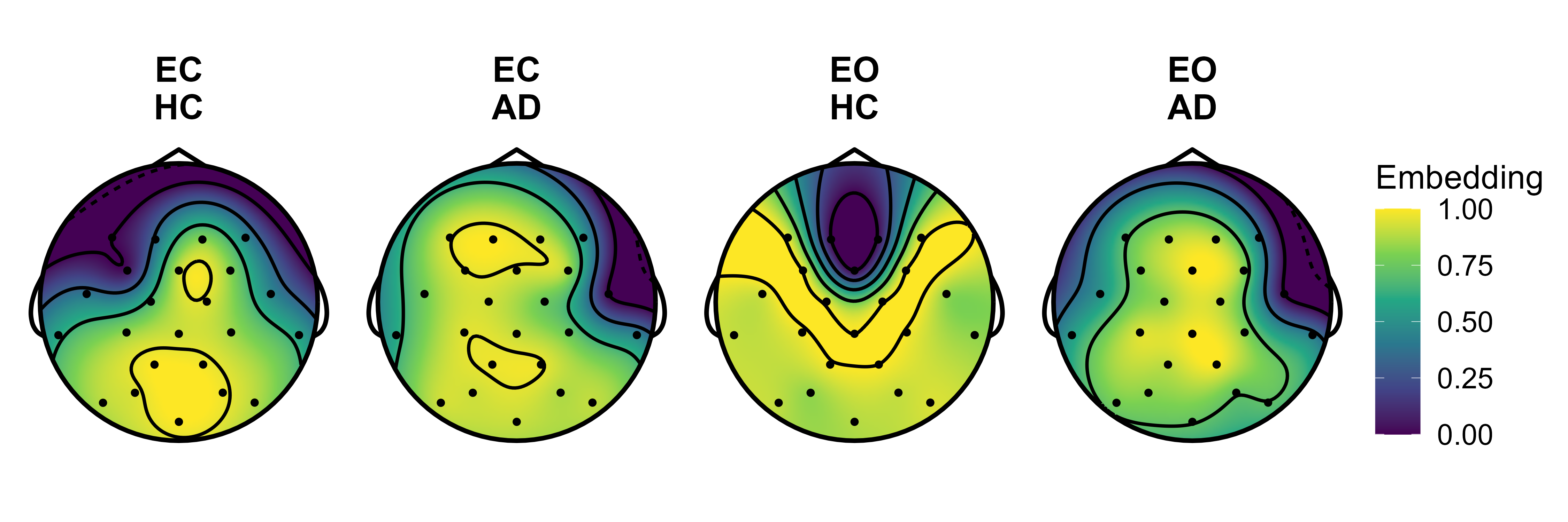
Another prediction explanation can be derived from the node embeddings obtained by the GGCN (Fig 5). In particular, we visualise the node embeddings obtained after four iterations of GGCN and compress them to 1D representation using principal component analysis (PCA) and extracting the first principal component. PCA is fitted for each condition separately. The node embeddings do not express a change in activity but rather a node similarity. Generally, the node embedding explanations show two large regions of similar embeddings. In EC, these are frontotemporal and centro-parietal regions, and right frontotemporal and the rest of the regions for HC and AD, respectively. The HC similarity region in the EO condition is reduced from frontotemporal to only the frontal region. In contrast, the AD similarity region expands from the right frontotemporal region to the left side. This further highlights the differences in learned patterns under the EC and EO conditions, thus explaining the reduced performance in the combined EC+EO condition.
Next, the role of the gating mechanism is elucidated by analysing the amount of information gathered at each scale, i.e. iteration of GGCN (Fig. 6). We measure this by computing the average Euclidean distance between the initial and updated node embedding at each iteration, i.e. and in Eq. 3. For instance, a small distance means a small amount of information was gathered at that scale. Local information contributes highly to the node embeddings of the AD cases, and then the degree of contributions linearly decreases with increasing graph scale. The opposite pattern is observed for HC cases, where the later iterations influence the node embeddings. This highlights the degradation of global and distributed information caused by AD since the model can efficiently learn with fewer iterations, i.e. most information is obtained from the first three iterations.




IV.3.3 Node pooling module
The node pooling mechanism can be exploited to derive two explanations. First, we analyse the frequency with which each node is included in the coarsened graph, i.e. pooling frequency (Fig. 7). Second, cluster attention scores (i.e. in Eq. 5) can be used to identify important hubs that are highly represented in the clusters learned by the node pooling module (Fig. 8).
The nodes in parieto-occipital regions are consistently selected with high pooling frequency for AD and HC cases across both EC and EO conditions (Fig. 7). Additionally, in EC condition, HC cases frequently select frontal nodes while AD cases tend to select central nodes. In contrast, in the EO condition, there seems to be more variation in the pooling frequency, with temporal nodes having a high pooling frequency for AD and HC cases.
Note that the nodes of the pooled graphs are, in fact, cluster embeddings, i.e. attention weighted sum of node embeddings (Eq. 7). We visualise the nodes with the highest attention scores of each cluster to highlight important hubs (Fig. 8). The attention scores are directed edges from a source node, transferring information to the cluster centred at the target node. Alternatively, these scores can be interpreted as a cluster membership strength. This information transfer should be interpreted as information flow within the model and most likely does not reflect an information flow within the brain.
In EC, AD cases show a large hub at the P4PZ node with strong long-distance and short-distance to various nodes. Additionally, there is a smaller hub at the T5O1. Similarly, in EO, AD cases have a large hub at the T3C3 node and a smaller one at the T4T6 node. In contrast, HC cases do not have any apparent hubs in the EC condition, with only a small hub at the P4PZ node. The attention links also seem to be rather short-distance. In the EO condition, HC cases show a large hub at the T6O2 node and smaller hubs at the P4PZ and T4T6 nodes.
This variance between EC and EO conditions displayed in the pooling frequency and attention scores suggests a plausible answer to why it is challenging for the model to learn joint representation in the EC+EO combined condition. We speculate this is caused by the additional dynamics introduced by the visual processing during the EO condition.
IV.3.4 Feature masking
We utilise feature masking to elucidate the importance of the frequency components summarised at each node by the node feature vector, i.e. PSD. In this, values at a selected part of the node feature vectors are replaced by zeroes and the model is retrained on this modified dataset. The relative reduction in f1 scores was then measured and visualised in Fig 9 for EC and EO conditions.
In both EC and EO conditions, the frequencies between 6 and 10 Hz are the most important since their masking reduced performance by 4.82% and 9.18%, respectively. This fits well with the well-described increase of power as well as functional connectivity in AD within these frequencies corresponding to and low bands babiloni2016synchronisationreview; klepl2022bispectrum. Similarly, masking of the , and frequency ranges results in a significant performance decrease in both EC and EO. Additionally, in EO condition, the , and frequency ranges produce a significant performance decrease.

IV.4 Limitations and future work
Although our approach achieves competitive performance, we identify a few drawbacks. First, the relatively small size of our dataset imposes a limit on fitting complex models. We address this issue by segmenting the EEG signals into short windows. The short window length means that the model might not be able to represent information from low-frequency components of the signal.
Next, we do not explore alternative node feature representations beyond PSD in this study. PSD is merely a linear frequency-domain representation of the signal. Including time-domain and nonlinear information in the node features might improve the expressiveness of the model. Similarly, the proposed graph learning mechanism is limited to linear coupling patterns because (1) it is inferred from the node features and (2) it is expressed as Pearson’s correlation coefficient. Future work should explore other forms of FC that might be integrated into the graph learning mechanism and study ways to include more complex frequency-dependent coupling information.
Finally, the model architecture might be limited by the relatively large number of hyper-parameters that need to be optimised. However, this limitation should be mitigated by utilising a validation set during the optimisation. Moreover, we explore the model stability with respect to some of the important hyperparameters in the parameter sensitivity experiments. These suggest that the achieved performance of the proposed model is not limited purely to the optimal values of the hyperparameters.
V Conclusion
This work proposes a novel graph learning model that performs highly in the AD diagnosis task. Additionally, we show that the model produces robust and clinically relevant explanations for its predictions via the novel graph structure learning module and the node pooling mechanism. Finally, we highlight the importance of utilising the gating mechanism within a message-passing encoder. This allows the model to accurately represent the multiscale distributed network disruptions displayed in the AD cases.
Acknowledgement
The EEG data was funded by a grant from Alzheimer’s Research UK (ARUK-PPG20114B-25). The views expressed are those of the author(s) and not necessarily those of the NHS, the NIHR or the Department of Health. The work was supported by A*STAR, AI, Analytics and Informatics (AI3) Horizontal Technology Programme Office (HTPO) seed grant C211118015.
References
- [1] Xavier Delbeuck, Martial Van der Linden, and Fabienne Collette. Alzheimer’disease as a disconnection syndrome? Neuropsychology review, 13(2):79–92, 2003.
- [2] Willem de Haan, Wiesje M van der Flier, T Koene, Lieke L Smits, Philip Scheltens, and Cornelis J Stam. Disrupted modular brain dynamics reflect cognitive dysfunction in Alzheimer’s disease. Neuroimage, 59(4):3085–3093, 2012.
- [3] Michela Pievani, Willem de Haan, Tao Wu, William W Seeley, and Giovanni B Frisoni. Functional network disruption in the degenerative dementias. The Lancet Neurology, 10(9):829–843, 2011.
- [4] Thomas König, L Prichep, Thomas Dierks, Daniela Hubl, LO Wahlund, ER John, and V Jelic. Decreased eeg synchronization in alzheimer’s disease and mild cognitive impairment. Neurobiology of aging, 26(2):165–171, 2005.
- [5] Richard Mayeux and Yaakov Stern. Epidemiology of alzheimer disease. Cold Spring Harbor perspectives in medicine, 2(8):a006239, 2012.
- [6] Paolo Maria Rossini, Riccardo Di Iorio, Francesco Vecchio, Maria Anfossi, Claudio Babiloni, M Bozzali, Amalia Cecilia Bruni, Stefano F Cappa, Julien Escudero, Francisco Jose Fraga, et al. Early diagnosis of alzheimer’s disease: the role of biomarkers including advanced eeg signal analysis. report from the ifcn-sponsored panel of experts. Clinical Neurophysiology, 131(6):1287–1310, 2020.
- [7] Claudio Babiloni, Roberta Lizio, Nicola Marzano, Paolo Capotosto, Andrea Soricelli, Antonio Ivano Triggiani, Susanna Cordone, Loreto Gesualdo, and Claudio Del Percio. Brain neural synchronization and functional coupling in alzheimer’s disease as revealed by resting state eeg rhythms. International Journal of Psychophysiology, 103:88–102, 2016.
- [8] Dominik Klepl, Fei He, Min Wu, Daniel J Blackburn, and Ptolemaios Sarrigiannis. EEG-based graph neural network classification of alzheimer’s disease: An empirical evaluation of functional connectivity methods. IEEE Transactions on Neural Systems and Rehabilitation Engineering, 30:2651–2660, 2022.
- [9] Dominik Klepl, Fei He, Wu Min, Daniel Blackburn, and Ptolemaios Sarrigiannis. Bispectrum-based cross-frequency functional connectivity: Classification of alzheimer’s disease. In 2022 44th Annual International Conference of the IEEE Engineering in Medicine & Biology Society (EMBC), pages 305–308. IEEE, 2022.
- [10] Dominik Klepl, Fei He, Min Wu, Matteo De Marco, Daniel J Blackburn, and Ptolemaios G Sarrigiannis. Characterising alzheimer’s disease with eeg-based energy landscape analysis. IEEE Journal of Biomedical and Health Informatics, 26(3):992–1000, 2021.
- [11] Xiaocai Shan, Jun Cao, Shoudong Huo, Liangyu Chen, Ptolemaios Georgios Sarrigiannis, and Yifan Zhao. Spatial–temporal graph convolutional network for alzheimer classification based on brain functional connectivity imaging of electroencephalogram. Human Brain Mapping, 2022.
- [12] Sou Nobukawa, Teruya Yamanishi, Shinya Kasakawa, Haruhiko Nishimura, Mitsuru Kikuchi, and Tetsuya Takahashi. Classification methods based on complexity and synchronization of electroencephalography signals in alzheimer’s disease. Frontiers in psychiatry, 11:255, 2020.
- [13] Saman Fouladi, Ali A Safaei, Nadia Mammone, Foad Ghaderi, and MJ Ebadi. Efficient deep neural networks for classification of alzheimer’s disease and mild cognitive impairment from scalp eeg recordings. Cognitive Computation, pages 1–22, 2022.
- [14] Jaeseung Jeong. Eeg dynamics in patients with alzheimer’s disease. Clinical neurophysiology, 115(7):1490–1505, 2004.
- [15] Dominik Klepl, Fei He, Min Wu, Daniel J Blackburn, and Ptolemaios G Sarrigiannis. Cross-frequency multilayer network analysis with bispectrum-based functional connectivity: A study of alzheimer’s disease. bioRxiv, pages 2021–08, 2021.
- [16] Parham Ghorbanian, David M Devilbiss, Terry Hess, Allan Bernstein, Adam J Simon, and Hashem Ashrafiuon. Exploration of eeg features of alzheimer’s disease using continuous wavelet transform. Medical & biological engineering & computing, 53(9):843–855, 2015.
- [17] Kaustubh Supekar, Vinod Menon, Daniel Rubin, Mark Musen, and Michael D Greicius. Network analysis of intrinsic functional brain connectivity in Alzheimer’s disease. PLoS Comput Biol, 4(6):e1000100, 2008.
- [18] A Kabbara, H Eid, W El Falou, M Khalil, F Wendling, and M Hassan. Reduced integration and improved segregation of functional brain networks in Alzheimer’s disease. Journal of neural engineering, 15(2):026023, 2018.
- [19] Fabrizio Vecchio, Francesca Miraglia, Francesca Alú, Alessandro Orticoni, Elda Judica, Maria Cotelli, and Paolo Maria Rossini. Contribution of graph theory applied to EEG data analysis for Alzheimer’s disease versus vascular dementia diagnosis. Journal of Alzheimer’s Disease, 82(2):871–879, 2021.
- [20] Cornelis J Stam, BF Jones, G Nolte, M Breakspear, and Ph Scheltens. Small-world networks and functional connectivity in Alzheimer’s disease. Cerebral cortex, 17(1):92–99, 2007.
- [21] Burcu Oltu, Mehmet Feyzi Akşahin, and Seda Kibaroğlu. A novel electroencephalography based approach for alzheimer’s disease and mild cognitive impairment detection. Biomedical Signal Processing and Control, 63:102223, 2021.
- [22] Zhenxi Song, Bin Deng, Jiang Wang, and Ruofan Wang. Biomarkers for alzheimer’s disease defined by a novel brain functional network measure. IEEE Transactions on Biomedical Engineering, 66(1):41–49, 2018.
- [23] Haitao Yu, Xinyu Lei, Zhenxi Song, Chen Liu, and Jiang Wang. Supervised network-based fuzzy learning of eeg signals for alzheimer’s disease identification. IEEE Transactions on Fuzzy Systems, 28(1):60–71, 2019.
- [24] Cosimo Ieracitano, Nadia Mammone, Alessia Bramanti, Amir Hussain, and Francesco C Morabito. A convolutional neural network approach for classification of dementia stages based on 2d-spectral representation of eeg recordings. Neurocomputing, 323:96–107, 2019.
- [25] L Dharshana Deepthi, D Shanthi, and M Buvana. An intelligent alzheimer’s disease prediction using convolutional neural network (cnn). International Journal of Advanced Research in Engineering and Technology (IJARET), 11(4):12–22, 2020.
- [26] Xiaojun Bi and Haibo Wang. Early alzheimer’s disease diagnosis based on eeg spectral images using deep learning. Neural Networks, 114:119–135, 2019.
- [27] Cameron J Huggins, Javier Escudero, Mario A Parra, Brian Scally, Renato Anghinah, Amanda Vitória Lacerda De Araújo, Luis F Basile, and Daniel Abasolo. Deep learning of resting-state electroencephalogram signals for three-class classification of alzheimer’s disease, mild cognitive impairment and healthy ageing. Journal of Neural Engineering, 18(4):046087, 2021.
- [28] Caroline L Alves, Aruane M Pineda, Kirstin Roster, Christiane Thielemann, and Francisco A Rodrigues. Eeg functional connectivity and deep learning for automatic diagnosis of brain disorders: Alzheimer’s disease and schizophrenia. Journal of Physics: Complexity, 3(2):025001, 2022.
- [29] Rui Li, Yiting Wang, and Bao-Liang Lu. A multi-domain adaptive graph convolutional network for eeg-based emotion recognition. In Proceedings of the 29th ACM International Conference on Multimedia, pages 5565–5573, 2021.
- [30] Shiva Asadzadeh, Tohid Yousefi Rezaii, Soosan Beheshti, and Saeed Meshgini. Accurate emotion recognition using bayesian model based eeg sources as dynamic graph convolutional neural network nodes. Scientific Reports, 12(1):1–14, 2022.
- [31] Lu-Bao LI, Tian CHEN, Fu-Ji REN, and Bei-Bei LUO. Bimodal emotion recognition method based on graph neural networks and attention. Journal of Computer Applications, page 0, 2022.
- [32] Khadijeh Raeisi, Mohammad Khazaei, Pierpaolo Croce, Gabriella Tamburro, Silvia Comani, and Filippo Zappasodi. A graph convolutional neural network for the automated detection of seizures in the neonatal eeg. Computer Methods and Programs in Biomedicine, page 106950, 2022.
- [33] Siyi Tang, Jared Dunnmon, Khaled Kamal Saab, Xuan Zhang, Qianying Huang, Florian Dubost, Daniel Rubin, and Christopher Lee-Messer. Self-supervised graph neural networks for improved electroencephalographic seizure analysis. In International Conference on Learning Representations, 2021.
- [34] Mingyi Sun, Weigang Cui, Shuyue Yu, Hongbin Han, Bin Hu, and Yang Li. A dual-branch dynamic graph convolution based adaptive transformer feature fusion network for eeg emotion recognition. IEEE Transactions on Affective Computing, 2022.
- [35] Yongqiang Yin, Xiangwei Zheng, Bin Hu, Yuang Zhang, and Xinchun Cui. Eeg emotion recognition using fusion model of graph convolutional neural networks and lstm. Applied Soft Computing, 100:106954, 2021.
- [36] Jianhui Chen, Hui Qian, and Xiaoliang Gong. Bayesian graph neural networks for eeg-based emotion recognition. In Clinical Image-Based Procedures, Distributed and Collaborative Learning, Artificial Intelligence for Combating COVID-19 and Secure and Privacy-Preserving Machine Learning, pages 24–33. Springer, 2021.
- [37] Ziyu Jia, Youfang Lin, Jing Wang, Ronghao Zhou, Xiaojun Ning, Yuanlai He, and Yaoshuai Zhao. Graphsleepnet: Adaptive spatial-temporal graph convolutional networks for sleep stage classification. In IJCAI, pages 1324–1330, 2020.
- [38] Hong Zeng, Qi Wu, Yanping Jin, Haohao Zheng, Mingming Li, Yue Zhao, Hua Hu, and Wanzeng Kong. Siam-gcan: a siamese graph convolutional attention network for eeg emotion recognition. IEEE Transactions on Instrumentation and Measurement, 2022.
- [39] Hanjie Liu, Jinren Zhang, Qingshan Liu, and Jinde Cao. Minimum spanning tree based graph neural network for emotion classification using eeg. Neural Networks, 145:308–318, 2022.
- [40] Qi Chang, Cancheng Li, Qing Tian, Qijing Bo, Jicong Zhang, Yanbing Xiong, and Chuanyue Wang. Classification of first-episode schizophrenia, chronic schizophrenia and healthy control based on brain network of mismatch negativity by graph neural network. IEEE Transactions on Neural Systems and Rehabilitation Engineering, 29:1784–1794, 2021.
- [41] Xiaoyu Li, Buyue Qian, Jishang Wei, An Li, Xuan Liu, and Qinghua Zheng. Classify eeg and reveal latent graph structure with spatio-temporal graph convolutional neural network. In 2019 IEEE International Conference on Data Mining (ICDM), pages 389–398. IEEE, 2019.
- [42] Peixiang Zhong, Di Wang, and Chunyan Miao. Eeg-based emotion recognition using regularized graph neural networks. IEEE Transactions on Affective Computing, 2020.
- [43] Maksim Zhdanov, Saskia Steinmann, and Nico Hoffmann. Investigating brain connectivity with graph neural networks and gnnexplainer. arXiv preprint arXiv:2206.01930, 2022.
- [44] Yujia Li, Richard Zemel, Marc Brockschmidt, and Daniel Tarlow. Gated graph sequence neural networks. In Proceedings of ICLR’16, 2016.
- [45] Ekagra Ranjan, Soumya Sanyal, and Partha Talukdar. Asap: Adaptive structure aware pooling for learning hierarchical graph representations. In Proceedings of the AAAI Conference on Artificial Intelligence, volume 34, pages 5470–5477, 2020.
- [46] Tao Xu, Wang Dang, Jiabao Wang, and Yun Zhou. Dagam: A domain adversarial graph attention model for subject independent eeg-based emotion recognition. arXiv preprint arXiv:2202.12948, 2022.
- [47] Andac Demir, Toshiaki Koike-Akino, Ye Wang, Masaki Haruna, and Deniz Erdogmus. Eeg-gnn: Graph neural networks for classification of electroencephalogram (eeg) signals. In 2021 43rd Annual International Conference of the IEEE Engineering in Medicine & Biology Society (EMBC), pages 1061–1067. IEEE, 2021.
- [48] Daniel J. Blackburn, Yifan Zhao, Matteo De Marco, Simon M. Bell, Fei He, Hua-Liang Wei, Sarah Lawrence, Zoe C. Unwin, Michelle Blyth, and Jenna Angel. A pilot study investigating a novel non-linear measure of eyes open versus eyes closed eeg synchronization in people with Alzheimer’s disease and healthy controls. Brain sciences, 8(7):134, 2018.
- [49] Kyunghyun Cho, Bart Van Merriënboer, Dzmitry Bahdanau, and Yoshua Bengio. On the properties of neural machine translation: Encoder-decoder approaches. arXiv preprint arXiv:1409.1259, 2014.
- [50] Adam Paszke, Sam Gross, Francisco Massa, Adam Lerer, James Bradbury, Gregory Chanan, Trevor Killeen, Zeming Lin, Natalia Gimelshein, Luca Antiga, Alban Desmaison, Andreas Kopf, Edward Yang, Zachary DeVito, Martin Raison, Alykhan Tejani, Sasank Chilamkurthy, Benoit Steiner, Lu Fang, Junjie Bai, and Soumith Chintala. PyTorch: An imperative style, high-performance deep learning library. In Advances in Neural Information Processing Systems 32, pages 8024–8035. 2019.
- [51] Matthias Fey and Jan E. Lenssen. Fast graph representation learning with PyTorch Geometric. In ICLR Workshop on Representation Learning on Graphs and Manifolds, 2019.
- [52] Christian Sandøe Musaeus, Knut Engedal, Peter Høgh, Vesna Jelic, Morten Mørup, Mala Naik, Anne-Rita Oeksengaard, Jon Snaedal, Lars-Olof Wahlund, Gunhild Waldemar, and Birgitte Bo Andersen. Oscillatory connectivity as a diagnostic marker of dementia due to Alzheimer’s disease. Clinical Neurophysiology, 130(10):1889–1899, October 2019.
Appendix A Hyperparameters of proposed model
The optimised and allowed values of the various hyperparameters of the proposed adaptive gated graph convolutional network (AGGCN) are reported in Tables 3 and 4, respectively.
| kernel size | CNN filters | ||||
|---|---|---|---|---|---|
| 1 | 4 | 84 | 403 | 0.024 | 16 |
| activation | aggregation | ||||
| 4 | 372 | Tanh | mean | 0.9 | |
| negative slope | |||||
| 3 | 0.75 | 0.085 | 3 | 16 | 0 |
| learning rate | momentum | weight decay | |||
| 0.063 | 0.859 | 0.076 | 0.896 | 0.346 | 0.1 |
| Hyperparameter | Values |
|---|---|
| kernel size | |
| CNN filters | |
| activation | |
| aggregation | |
| negative slope | |
| learning rate | |
| momentum | |
| weight decay | |
Appendix B Parameter sensitivity experiments
Multiple parameter sensitivity experiments were performed to test the influence of the selected crucial hyperparameters of AGGCN. The results of these experiments are reported in Figures 10, 11, 12 and 13 for the number of GGCN iterations, K-nearest neighbour edges kept in the sparse learned graph structure, size of the coarsened (pooled) graph and aggregation function, respectively.


Appendix C Explainability of AGGCN: Adjacency-based visualisations
The main manuscript shows the AGGCN-learned graphs and the node pooling patterns as a graph. In order to facilitate a different view of the same results, we report the averaged adjacency matrices in Figure 14 that correspond to Figure 3 in the main text. Similarly, we report the differences between the learned graphs together with effect sizes (Wilcox permutation effect size) to quantify the strength of these differences (Figure 15, corresponding to Figure 4 in the main text). Finally, we report an adjacency-like view of the node pooling attention scores (Figure 16) corresponding to Figure 8 in the main text.


(B) The effect size for the non-parametric Mann-Whitney U tests comparing AD and HC with values set to 0 where ,
