Quantum-enhanced pattern recognition
Abstract
The challenge of pattern recognition is to invoke a strategy that can accurately extract features of a dataset and classify its samples. In realistic scenarios this dataset may be a physical system from which we want to retrieve information, such as in the readout of optical classical memories. The theoretical and experimental development of quantum reading has demonstrated that the readout of optical memories can be dramatically enhanced through the use of quantum resources (namely entangled input-states) over that of the best classical strategies. However, the practicality of this quantum advantage hinges upon the scalability of quantum reading, and up to now its experimental demonstration has been limited to individual cells. In this work, we demonstrate for the first time quantum advantage in the multi-cell problem of pattern recognition. Through experimental realizations of digits from the MNIST handwritten digit dataset, and the application of advanced classical post-processing, we report the use of entangled probe states and photon-counting to achieve quantum advantage in classification error over that achieved with classical resources, confirming that the advantage gained through quantum sensors can be sustained throughout pattern recognition and complex post-processing. This motivates future developments of quantum-enhanced pattern recognition of bosonic-loss within complex domains.
Significant progress has been made in recent years in quantum sensing Degen et al. 2017; Pirandola et al. 2018; Petrini et al. 2020, a broad spanning field of research which seeks to realise quantum protocols for estimation Helstrom 1976; Braunstein and Caves 1994; Braunstein et al. 1996; Giovannetti et al. 2004; Giovannetti et al. 2011 and discrimination Helstrom 1969; Chefles and Barnett 1998; Chefles 2000; Bergou et al. 2004 that achieve better performance than any classical protocol, i.e. gain a quantum-advantage. Efforts to design and engineer such protocols have been widely successful, with applications in data-readout Pirandola 2011; Pirandola et al. 2011; Nair 2011; Invernizzi et al. 2011; Dall’Arno et al. 2012; Spedalieri et al. 2012; Tej et al. 2013; Ortolano et al. 2021a; Ortolano et al. 2021b; Ortolano and Ruo-Berchera 2022, target detection Sacchi 2005; Lloyd 2008; Tan et al. 2008; Lopaeva et al. 2013; Zhang et al. 2013; Zhang et al. 2015; Barzanjeh et al. 2015; Sanz et al. 2017; Zhuang et al. 2017a; Zhuang et al. 2017b; Barzanjeh et al. 2020; Casariego et al. 2022; Zhuang and Shapiro 2022; Gonzalez-Raya and Sanz 2022, cryptography Spedalieri 2015; Pereira and Pirandola 2021, fundamental physics research Brady et al. 2022; Marchese et al. 2021; Ruo Berchera et al. 2013 and imaging Genovese 2016; Losero et al. 2018; Spedalieri et al. 2020.
An application of particular interest is that of quantum reading, which encompasses the challenge of classical information retrieval from an optical memory. A memory cell can be considered as a reflective (or transmissive) target with two distinct possible reflectivities (transmittivities) encoding a classical bit. This represents a pair of possible bosonic-lossy channels that act on incident photonic probe states. Accurate readout of a memory cell requires the correct discrimination of output states from the channel (i.e., quantum channel discrimination). Having conceptualised this model, Pirandola Pirandola 2011 proved that one can significantly enhance the accuracy of information retrieval through the use of entangled light sources. This seminal work led to a series of advancements and most recently, a successful experimental demonstration Ortolano et al. 2021a.
The success of quantum reading prompted the development of further schemes in more complex domains, such as the simultaneous readout of many memory cells. This breeds the task of quantum multi-channel discrimination Zhuang and Pirandola 2020a; Zhuang and Pirandola 2020b, in which one must optimise multi-mode probe states and measurements in order to classify a collection of bosonic-lossy channels (or channel patterns). This development brings new layers of complication; expanding the space of possible channel patterns to be discriminated, and revealing a more general spectrum of multi-modal discrimination protocols. This invites new applications in which quantum reading may serve as a primitive.
The use of quantum sensors within the task of pattern recognition provides such an opportunity, where one is tasked with classifying a set of patterns (or images). The pattern distribution is often non-uniform, and classifications follow highly non-linear relationships, e.g. the classification of hand-written digits. Powerful classical post-processing techniques are well known for this challenge, however the quality of the readout of data-sets are often taken for granted. Given a system that can be modelled as an ensemble of bosonic-lossy multi-channels, it has been theoretically shown that quantum reading can substantially enhance classification power over optimal classical strategies Banchi et al. 2020; Pereira et al. 2020; Harney et al. 2021; Harney and Pirandola 2021a; Harney and Pirandola 2021b.
In this work, we report the experimental demonstration of quantum-enhanced pattern recognition using signal-idler entangled two-mode squeezed vacuum (TMSV) states and photon-counting measurements to outperform any classical strategy. Using the MNIST handwritten digit dataset Lecun et al. 1998, image samples are experimentally realised and serve as a test-bed for the discrimination protocols. Investigating both multi-shot and single-shot regimes, we show that the use of entangled probe states can generate quantum advantage in the classification error as a consequence of the gain offered by quantum resources. By considering multiple supervised-learning approaches to classification, we emphasise that this advantage is an inherent property of quantum sensing that can survive throughout complex post-processing. Our work paves the way for a suite of near-term applications of quantum-enhanced pattern recognition and imaging.
I Results
Let us consider a pattern classification problem where spatial patterns are imprinted on a array of binary cells, each encoding one bit of information in two values of a physical parameter, for example the transmittances and , where we pose (see Fig. 1A). The cells size and dimension of the array , can be a native characteristic of the physical support but also they can be practically determined by resolution properties of the sensing apparatus, for example the pixel structure of a camera or the resolution of an optical system, so that and are intended as the values corresponding to each readout pixel. The sensing strategy has to be designed to minimize the average classification error probability of the patterns, .
The general sensing procedure can be described as in Fig. 1A: an input state, represented by the density operator , interacts with the object encoding the pattern, and a POVM measurement is performed on the output state, followed by classical post-processing. The state is generally bipartite in order to include ancillary assisted schemes. The two systems are indicated as signal (S) and idler (I), according to quantum optics terminology. Since we are dealing with bosonic systems, the problem is non-trivial only if we impose some constraints on the resources, the most natural one being to fix the mean number of signal photons, , probing the cell. The pixels are assumed to be probed by independent spatial modes, and in this work we restrict our analysis to local measurements, i.e. independent readout is performed for each pixel at the receiver.
Following the local measurement, a binary value is assigned to each pixel with a certain average probability of error . The binary image is then classified. The classification error is related to the bit-flip probability by a, generally, non-linear map :
| (1) |
The map depends on the problem at hand, but it is reasonable to assume it monotonic for any effective classification algorithm. Using the monotonicity of , the minimization of is obtained by minimizing over all possible input states and POVM measurements. Details on the single-pixel problem are provided in Sec. III.1.

The theoretical lower bound on the error probability achievable by classical states, is reported in Eq. (3). It can be saturated, without idler assistance, by a single mode coherent state , and an optimal measurement consisting in the projection on two pseudo-cat states as shown in Sec. III.2.
Such a measurement appears to be experimentally unfeasible and no other receiver that saturates has been proposed so far. Nevertheless, a photon counting (PC) receiver, composed of PC measurement followed by a Bayesian decision, can be proven to perform close to the optimal one for practical purposes Ortolano et al. 2021a. As the PC is a phase-insensitive measurement, it follows that any state with Poisson photon number distribution can reach the PC limit, , as reported in Eq. (6). For this reason, we use a PC receiver to experimentally perform the pixel readout with both classical and quantum states.
The quantum readout was performed using a collection of replicas of TMSV states, , with
| (2) |
is the thermal distribution with mean photons. In the quantum case, idler assistance is crucial and it is actually convenient to spread the signal energy across a large number of modes, i.e. to work with and Ortolano et al. 2021a. The corresponding error probability , discussed in Sec. III.1, can be evaluated numerically.
Among the various experimental imperfections, the most relevant is photon loss due to non-ideal optical component and detector inefficiency. The effect of the losses on classical readout performances is equivalent to a rescaling of the energy, namely the input mean photon number is substituted by the detected photons, in the classical bounds of Eqs. (3) and (6), where is the overall photon detection probability. However, the quantum strategy is additionally affected by deterioration of the bipartite non-classical correlation due to losses, which describes the imperfect coupling of correlated modes into the detectors. This effect is discussed in Sec. I.3.
I.1 Experimental realization
The principle of the experimental scheme is presented in Fig. 1 B-C. The -product TMSV quantum state is produced by traveling wave Spontaneous Parametric Down Conversion (SPDC) of type II in a non-linear crystal pumped by a continuous laser. Due to the conservation of the transverse momentum of the pump , it follows , i.e. signal and idler photons are emitted along correlated directions (spatial modes), which are mapped into symmetric pixels of a CCD camera. In our experiment the exposure time of image acquisition is much longer than the coherence time of the process, so many temporal modes, on the order of , contribute to the total number of photons detected in each pixel (few thousands). Clearly, the conditions and which maximize the quantum advantage are fulfilled and the single pixel photon statistics is practically indistinguishable from the Poisson one. For this reason, the best classical performance with PC detection can be evaluated by considering only the signal beam. Details on the experimental setup are reported in Sec. III.5.
In general, traveling wave SPDC is spatially broadband. There are many (several thousands) pairwise correlated spatial modes available for spatially resolved multi-pixel quantum readout Brida et al. 2010; Samantaray et al. 2017. However, a trade-off should be set between the spatial resolution, in terms of pixels available in one shot measurement, and the reduction of the pixel error probability due to quantum correlation. This point is discussed later on in the main text, and further details can be found in Sec. III.
To address this trade-off, we have realized the experiment in two different configurations, one named “scanning-like readout” (Fig. 1B) that favors the best quantum enhancement, and the second one named “multi-pixel readout” (Fig. 1C) that allows spatially resolved pattern acquisitions with in a single-shot measurement.
I.2 Scanning-Like Readout
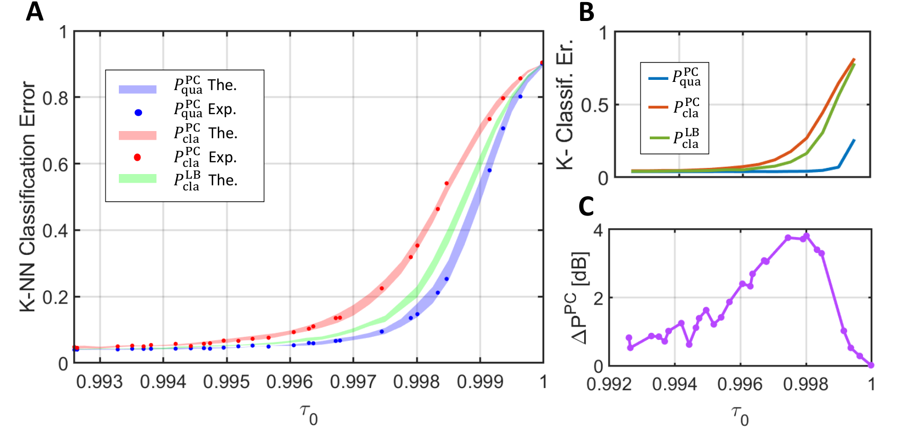
In this first experimental configuration, we mimic a readout in which the physical binary pattern encoded by the transmittance and is scanned point-by-point, as shown in Fig. 1B. First, we repeated a large number of independent measurements of two well-characterized transmittances, and , assigning a bit value for each measurement according to the Bayes’ rule in Eq. (4) based on the number of photon-counts and (see Sec. IIIA). The photon-counts are integrated over two large regions of the CCD array, defining the size of the readout pixel, collecting a large number of signal and idler spatial modes respectively, obtaining the best possible correlation between and , as discussed in Sec. IIID. This produces two sets of data and for the nominal transmittance and respectively, with . The procedure is performed both for classical (only using signal beam) and quantum reading. From those sets we can evaluate the average experimental readout pixel error probabilities, and shown in Fig. 2A. One of the transmittance is fixed to while the other one, , is varied. All other parameters are kept fixed. The experimental points for both the quantum (blue) and classical (red) readout are compared with the classical lower bound (green) defined by Eq. (3). As expected, in general the error probability increases as the two transmittances become closer and closer. However, through the range of parameters showed, the strategy employing quantum states sensibly outperforms the classical one paired with the suboptimal PC measurement and is also able to surpass the absolute classical lower bound. For the sake of completeness, in Fig. 2B we report the same pixel error probabilities in an almost ideal scenario where the detection efficiency is fixed to (the efficiency reached in the actual setup is ).

Note that, the data picked from the set and can be virtually rearranged to reproduce the outcomes of a sequential spatial scanning of any given binary pattern. However, for an accurate evaluation of the pattern recognition task, the used approach is highly preferable with respect to the real scanning of spatial samples. In fact, the last one would require the physical realization and scanning of a large number of spatial samples, which is hardly feasible and actually not necessary.
To evaluate the pattern recognition performance we used the MNIST handwritten digit dataset, containing 60000 training samples of handwritten numerical digits and 10000 test samples. We assemble the entire set of test patterns by picking experimental data from the set and . Fig. 3 shows some examples of digit contained in the dataset, and a comparison of the effect of the noise in either a classical and a quantum binary readout.
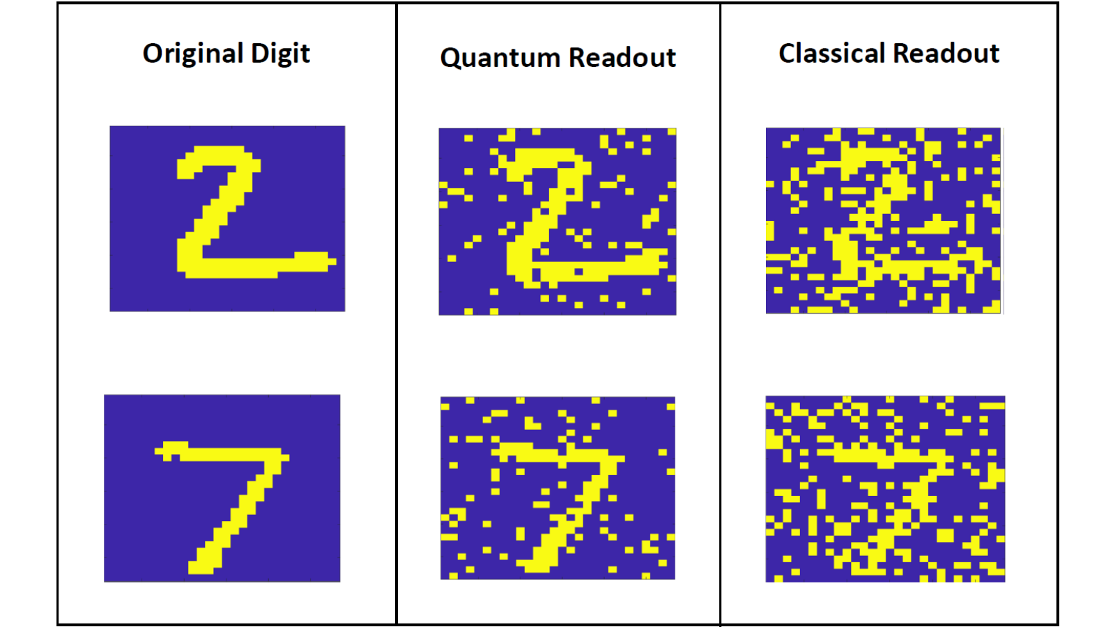
For the classification of the noisy digits we used a -Nearest Neighbor (-NN) classifier Cover and Hart 1967. A -NN classifier computes the distance between the pattern tested and all the patterns in its training set. In the case of binary patterns, the most natural metric is the Hamming distance. The closest patterns of the training set to the tested pattern are selected, and the class of the test pattern is assigned as the more common among the closest. The experimental classification error is reported in Fig. 4A as a function of the transmittance , while in Fig. 4B we report the classification performance in the almost ideal () detection scenario. Note that the performance of the -NN classifier is highly non-linear with respect to the single pixel error probability. For the values of corresponding to a classical error probability in Fig. 2A, the classification is very robust to noise. In this range, the classification error is almost negligible for all the strategies and the quantum advantage is also rather small. However, for higher transmittance , the algorithm becomes very sensitive to the readout noise level and here the advantage of quantum strategy is amplified. In fact, the experimental quantum advantage in the pattern recognition task, represented in Fig. 4C, reaches up to 4 dB, which is much larger than the corresponding pixel error improvement.
At this point, the question arises: is the amplification of the quantum advantage we have observed for the -NN classifier a property of this specific classifier, or a more general behavior characterizing the pattern classification task? To partially address this question, we repeat our analysis with another classification strategy that uses a refined machine learning approach.
Convolutional neural networks (CNNs) are a category of feed-forward neural networks that are omnipresent in the field of image processing, and are particularly powerful tool for pattern recognition O’Shea and Nash 2015; Gu et al. 2018. They contain hidden layers that convolve input data from one layer to the next, in which the convolutions are performed according to parameterised filters (or kernels). The goal of learning is to optimise these filters in such a way that complex features can be reliably extracted and classified. This form of network architecture helps to minimise the number of network parameters and also helps the CNN to interpret features in a translationally invariant way, i.e. qualities inferred in one area of an image can be reused elsewhere in the image.
In this work, we apply CNN classifiers to the task of noisy pattern recognition on the MNIST dataset as before with the -NN classifier, considering experimental input data from quantum-enhanced and classical sensors. We trained a collection of classifiers on a noisy training set in which each pixel in an image undergoes a bit flip with single-pixel error rate of , i.e. the single-pixel training error. Meanwhile, the network parameter optimisation was carried out by backpropagation using a cross-entropy loss cost function. More precisely, we prepared a set of 16 CNNs, whose was distributed across the interval . The single-pixel training error is a particularly influential parameter as fine-tuning helps classifiers become more robust to noise and learn how to reduce its impact on classification Nazaré et al. 2018. The classifiers could then be evaluated on the experimental test sets (constructed from and ) in order to quantify the performance of quantum-enhanced versus classical pattern recognition.
The results of the CNN strategy are presented in Fig. 5. Fig. 5A compares the performance of the classical and quantum-enhanced classifiers. We have a collection of CNN classifiers which have been trained using different single-pixel training errors, denoted by . It follows that some classifiers can garner better performance than others. Ideally, we would claim the classification error associated with the best classifier from our set, i.e. . But this approach remains unrealistic, since it is not possible to predict a priori what the best would be. Instead, we may use the single-pixel error rates associated with the chosen discrimination protocol to motivate our choice of training error rate at a given transmissivity , constructing the classifiers (for more details, see Sec. III.4). Fig. 5(b) plots these corresponding values against the single-pixel transmissivity.
Finally, Fig. 5(c) reports the quantum-advantage in the pattern recognition task (in decibels) showing a similar behaviour to the one observed in Fig. 4.C. This confirms that the quantum-advantage gathered through the single-pixel readout can be sustained throughout complex post-processing techniques, such as CNN training and evaluation.
I.3 Parallel Multi-Pixel Readout
While the scanning-like readout of the previous section represents a meaningful proof-of-principle necessary for a clean and faithful comparison with the theory, here we consider a more realistic scenario of a multi-pixel parallel readout, as it is depicted in Fig. 1C, where the pattern is acquired in single-shot.
The samples, containing digits from 0 to 9, were realized on a AR-coated glass slide combining laser lithography, sputtering deposition of titanium in high vacuum and lift off technique. The transmittance of the deposition is estimated as . The parallel readout is doable since the state produced by SPDC is spatially multimode. Pairwise correlated modes are detected by symmetric pairs of pixels in the CCD chip as represented in Fig. 1C, so that thousand pixel pairs are in principle non-classically correlated at the same time. However, to efficiently collect the correlated modes, the size of the pixel should be larger than the transverse cross-correlation length of the source. The consequence is a trade-off between the obtainable spatial resolution and the quantum advantage in the single pixel readout. We set the pixel size of our camera to fulfill the condition and at the same time to have a image of the digits (more details are presented in Sec IIID).
Fig. 6A shows the experimental pixel error probabilities for both classical an quantum PC readout in function of the effective transverse resolution at the sample plane. The effective resolution is changed by applying a moving averaging filter to the acquired images, as described in Sec IIID, which has practically the same effect of increasing the pixel size. On one side, the increasing of the pixel size has the direct consequence of raising the number of signal photons per pixel, that explains the dropping of classical error probability, according to Eq. (6). On the other side, as clearly shown in Fig. 6A, the quantum error probability decreases faster than the classical analogous, because the detectable quantum correlation increases while losing spatial resolution. Here, the comparison of the experimental results with the theoretical bounds is not straightforward and we will avoid it. In fact, when binary patterns are readout with finite resolution, for a detection pixel that falls across the edge between and the binary model is no longer valid. Such border effects are not negligible as the resolution decreases and become comparable with the the spatial features of the pattern. These features are very difficult to account for in a theoretical model.
We evaluated the pattern recognition performance once again on the MNIST handwritten digit dataset using a -NN algorithm for the classification. While the test dataset is composed of 10000 patterns, producing and acquiring samples is a not feasible and unnecessary task. In fact, the error in the classification can be broken down in two contributions. The first contribution is intrinsic to the classification algorithm and the second comes from the noise in the readout. In our case, with a pixel error larger than about 0.3, the classification error is dominated by the noise in sensing. For reference the classification error without noise is of the order of , while in the noisy region it is clearly much larger. So, we assume that the classification error can be well studied by printing a small subset of patterns from the original MNIST, namely 10, and performing on each of them one thousand different acquisitions with independent noise realizations, forming a total dataset of 10000 images.
The resulting classification error is reported in Fig. 6B as a function of the spatial resolution. The results are reported up to a resolution of 39 which is equivalent to an effective reduction of the resolution of a factor 3 with respect to the original dataset. Confirming the main results of the of the previous section, in a sensing scenario dominated by quantum noise, a relatively small quantum enhancement in the single pixel probability (namely from 0.35 to 0.32) can be amplified to around in the classification.
II Discussion and Conclusion
In this work we have experimentally demonstrated the advantage of quantum-enhanced sensing in the task of pattern recognition. As a test bed we have considered the problem of classification of handwritten digits. A quantum readout strategy based on TMSV states and photon counting measurement brings a relevant advantage in the classification errors with respect to any classical sensing.
We have realized the experiment in two different configurations. In the first one, called “scanning-like readout”, we have privileged the magnitude of the quantum advantage with respect to the acquisition time, since scanning of the sample is required. In this case we were able to clearly beat the optimal classical bound. In the second configuration, instead we have considered single-shot multi-pixel readout of the pattern. In this case we have shown a large advantage with respect to the classical bound that uses photon counting.
Moreover, the presence of quantum advantage turns out to be independent on complexity of the classification algorithm. Having deployed both -NN classifiers (a simple and robust strategy) and CNN classifiers (a machine learning enhanced strategy) on the same experimental data, similar results are obtained: quantum advantage in the sensing is maintained and often amplified in the pattern recognition task.
The results presented here are particularly promising for short terms application in biological spatial pattern recognition. In general, they also pave the way for experimental studies of quantum enhanced pattern recognition in the spectral and temporal domains.
III Materials & Methods
III.1 Single pixel readout
The single-pixel problem has been extensively analysed in Refs.Pirandola 2011; Invernizzi et al. 2011; Nair 2011; Ortolano et al. 2021a; Ortolano and Ruo-Berchera 2022. In the following we will compare three different local readout strategies. In the first scenario we consider classical input states , i.e. a mixture of coherent states, paired with a theoretical optimal POVM . The optimal probability of error in discriminating the outcome states and can be derived by the Helstrom bound Helstrom 1976, , where and are two generic states, and is the trace distance. Using the convexity of , Ref.Pirandola 2011 demonstrated the following bound to the classical error probability:
| (3) |
where is the mean number of signal photons. As discussed in Pirandola 2011, ancillary modes cannot enhance the performance of the readout with classical states, in fact the bound in Eq.(3) can be obtained by using a single mode coherent state transmitter , with , as shown in Sec. III.2.
However, the optimal measurement, that we discuss in Sec. III.2, is purely theoretical, and no feasible receiver has been proposed yet to reach the classical lower bound in Eq. (3). Thus, we consider a second, more practical scenario where the receiver is based on photon counting (PC) measurements that can be proven to perform close to the optimal one for practical purposes Ortolano et al. 2021a. The conditional photon number distribution at the receiver is , where is the number of measured photons in the signal and idler (the ancilla) systems. The optimal choice to recover the value of the bit is to choose it according to the Bayes’ rule
| (4) |
This condition is equivalent to the maximum likelihood decision in the balanced prior probability case. The error probability with photon counting receiver is given by:
| (5) |
i.e., proportional to the overlap of the measurement outcome distributions and . As for the optimal classical case, the conditional distribution overlap cannot be reduced by using ancillary mode, and the overlap is minimized for input signal states having the photon statistics of a coherent state, i.e. a Poisson distribution , where is the mean number of photons Ortolano et al. 2021a. The statistics of the photons returning from a cell of transmittance still follows the Poisson distribution, in particular . Substituting it in the conditional probabilities of Eq. (5), the best performance achievable with classical states and PC measurements is Ortolano et al. 2021a:
| (6) |
where is the incomplete gamma function, is the floor of and is the intersecting point of the two Poisson distributions and .
The third strategy we consider here uses a collection of replicas of Two Mode Squezed Vacuum (TMSV) states in input, , with and being a thermal distribution with mean photons. The joint probability of signal and idler photons of a TMSV state after the interaction with the cell of transmittance is , where stands for the binomial distribution. For the multi mode state the joint distribution is simply obtained by substituting the single mode thermal statistics with a multi-thermal one, , obtained by the convolution of thermal modes. The conditional joint probability evaluated in this way can be substituted in Eq. (5) to obtain the error of the quantum strategy, . This quantity can be evaluated numerically. It turns out that, for a fixed total number of photon transmitted to the cell , the most effective way to exploit quantum correlation is to span the photons in a large number of modes so that and . Moreover, the local multi-thermal distribution approaches the Poisson one. This is the regime that we consider in the simulation, and the one that is realized in the experiment.
III.2 Optimal local receiver for classical states
The single pixel readout probability of error that can be reached with classical states, having a fixed number of signal photons , is lower bounded by the limit in Eq. (3). As previously mentioned, this limit can be saturated by using a single-mode coherent state without idlers. This can be seen using the fact that a pure loss channel, with transmissivity , maps a coherent state into another, amplitude damped, coherent state . Once the input state is fixed, the discrimination of two channels having different transmissivity is reduced to a binary quantum state discrimination between the two possible outputs, and for which the lowest error probability is given by the Helstrom formula:
| (7) |
where is the trace distance and are the prior probabilities.
For coherent input, the potential outputs of the channel are pure and their trace distance can be expressed in terms of the overlap as:
Substituting this in Eq.(7) and setting equal priors we get:
| (8) |
which coincides with proving that a single mode coherent state saturates the classical bound (originally proven for an arbitrary P-representation Pirandola 2011).
The optimal probability of error is achieved by projecting into the eigenstates of the Hermitian operator:
| (9) |
We can find an orthogonal basis to represent by performing the Gram-Smith orthogonalization on the pair of vectors spanning its support. So we define the basis:
| (10) |
The eigenvectors of can be computed with simple algebra to be, in terms of this basis:
| (11) | ||||
| (12) |
And substituting the definitions in Eq.(10) leads to:
| (13) | ||||
| (14) |
The bit can then be recovered by measuring over the projectors and . Once the measurement is performed the value is selected if the outcome is and is selected otherwise. This measurement paired with a coherent state input would in theory saturate the classical bound in Eq.(3). However, as pointed out in the main text, from a practical point of view an implementation of this kind of measurement would be very complicated, if feasible at all, with current technology.
III.3 -NN classification
Let and , , be two binary images of dimension . The Hamming distance, , between and is defined as:
| (15) |
The -NN is a supervised classification method that uses the known label of images in a training set to assign a class to images in a test set . Given an image in , the set of its closest images in terms of the hamming distance, , are selected from . The image is assigned to the class which is the most common among the images in . The most intuitive case is given by the -NN classifier, that assigns to the image the same class of its closest image in the training set .
III.4 Neural Network classification
Consider a dataset of images in which each image possesses a classification (or label) . For the task of classification, a neural network Nielsen 2015; Murphy 2012 is a universal approximating function (where denotes the parameter set of the neural network) which takes an image as input and provides an approximation of its classification as an output, . Training a neural network as a classifier equates to optimising its parameters such that becomes a reliable classifier over the entire dataset. That is, the goal of training is to maximising the accuracy of the classifier over the training set in such a way that it can generalise to new, unforeseen samples. In a neural network, the parameter set describes correlations between layers of neurons, capable to encoding highly complex relationships between input and output.
When building neural network classifiers for which there already exists experimental data (as in the case of MNIST) supervised learning is a very effective strategy. This involves utilising a set of images whose classifications are already exactly known, and training the neural network on this data. In this way, the classifier can be optimised reliably and extract meaningful features from the dataset in order to learn correlations between input patterns and their classification. The classification error of the classifier is measured against an evaluation (or test) set; a set of images which the network has never seen during training and therefore must extrapolate. Given a -element evaluation set of images and labels and a classifier then the classification error is approximated as
| (16) |
where is a Kronecker-delta function that returns unity iff the classifications are the same, otherwise it will return zero.
In this work, we exploit CNNs as classifiers upon on our experimental dataset. Using the Julia Flux package Innes et al. 2018; Innes 2018, we construct CNNs with three convolutional layers and a dense layer, optimising a cross entropy loss function during training. This produces classifiers of sufficient accuracy to utilise in this study. We use the MNIST handwritten digit dataset, composed of a training set with images and an experimental evaluation set . The experimental dataset is clearly unchangeable and is inherently noisy. But the initially noiseless training set can be manipulated to modify and enhance our classifiers. As discussed in the main text, it is useful to train a CNN on noisy data if it is expected to classify noisy data. To do this, we simulate noisy training sets in which each pixel in every image is independently bit flipped according to the probability . We then trained a collection of different classifiers using different values of and evaluated them on the experimental data.
It is difficult to know what the best case is with respect to the transmissivity of the sampled pixels. As depicted in Fig. 5 we can identify a best choice classifier from our collection as that which minimises its classification error with respect to the evaluation set. However, it is not practical to select a best choice classifier a posteriori (this would defeat the purpose of discrimination). Instead, we present the best-case performance for benchmarking purposes and more practically motivate our chosen by mapping the single pixel transmissivity to a single-pixel error probability associated with the discrimination protocol being used.
III.5 Experimental Setup and Noise Reduction

Acquisitions for both the experimental configurations reported in Fig. 1B-C, are performed using the setup sketched in Fig. 7. It exploits SPDC to generate multi-mode pairwise correlated collections of TMSV states, by pumping a type II Beta Barium Borate (BBO) non-liner crystal with a 100 mW continuous laser at wavelength nm. The SPDC photons are selected around the degenerate wavelength nm by an interference filter (IF) at nm. The correlations in momentum at the source are converted in spatial correlations at the ”object” plane, by use of a lens having focal length , in an configuration, performing a Fourier transform on the incoming field. The test patterns to be classified are physically realized as depositions, according to the procedure of Sec. III.6. The patterns are placed in the signal beam at the object plane, while a blank glass slide is placed on the idler beam to match the two optical paths. The object plane is then imaged to the charged coupled device (CCD) camera using a second lens, with magnification of about 8 times. The camera (Princeton Instrument Pixis 400BR Excelon) has a nominal quantum efficiency , electronic noise of 4 and the physical pixel is of 13 m. The total channel efficiencies and , are estimated close to 80% according to the procedure outlined in Ref.s Brida et al. 2010; Avella et al. 2016
In the scanning-like configuration, we introduce in the signal beam a variable absorber that is fine tuned in the range . Signal and idler photons and are obtained integrating over two corresponding wide spatial areas composed of a large number of physical pixels, becoming equivalent to two bucket detectors. This leads to the most efficient collection of the correlated photons Ortolano et al. 2021b and thus to reach an higher quantum advantage, as we will explain in the following.
In contrast, in the parallel multi-pixel readout, we exploit the spatial resolution of the detector to have a one-shot (without scanning) image of size of a test digit in the signal arm, which is the original dimension of the binary images of the MNIST dataset. For that, we perform a hardware binning of the physical pixels, to obtain an effective readout pixel of m, corresponding to a resolution of m at the object plane (not to be confused with the original physical pixel size of the detector mentioned earlier).
However, a trade-off exists between spatial resolution and quantum noise reduction achieved exploiting the signal-idler correlations. Actually, correlated photons from the multi-mode SPDC arrive at the detector within a certain transverse spatial uncertainty, that comes from the finite size of the pump beam. For this reason, the signal-idler intensity cross-correlation is well approximated by a Gaussian function with finite coherence length at the detector plane (in our case is m). To efficiently detect the correlated modes, the pixel size, or more in general the detector resolution area, must be larger than this coherence length, Meda et al. 2017. In Sec.(I.3) we analyse the patter recognition performance as a function of the resolution. For a fair comparison in the classification, it is more suitable to have final binary images with always the same number of pixels. Thus, instead of changing the resolution by performing a simple pixel binning, we preferred to change it by applying an averaging filter of appropriate size. The averaging filter substitutes to each pixel count, the average of the counts in a neighborhood of size . This is repeated for each original pixel of the matrix, so that the final size of the image in terms of pixels is unvaried, although the effective spatial resolution is reduced. In the graph of Fig. 6A, the parameter ranges between 1 and 5, which correspond to an effective resolution between m and m. The improvement of the quantum correlations in function of the image resolution can be witnessed by the noise reduction factor (NRF), defined as Jedrkiewicz et al. 2004; Bondani et al. 2007; Blanchet et al. 2008; Agafonov et al. 2010; Peřina et al. 2012. The NRF is an indicator of non-classical correlations, since it can show values in the range only for non-classical fields, while it is for classical light. In Fig.(7.B) we report the measured NRF as a function of the effective resolution at the object plane.
III.6 Handwritten digit deposition
The CAD of the 10 digits (from 0 to 9) was realised by normalising the dimension of each binary images (28x28 pixels) of digit in squares of maximum dimension of 400x400 spaced of 1000 m. A laser lithography process was performed with Heidelberg Instruments uPG101 system equipped with a UV laser source at 375 nm. The deposition of titanium was carried out by sputtering in high vacuum at low rate (0,08 nm/s). Thicknesses from 2 to 4 nm were deposited to obtain a transmittance value suitable for the experiment. Final patterning was obtained removing titanium excess through lift off technique.
Acknowledgments
Part of this work (sample fabrication) has been carried out at QR Laboratories, INRiM, a micro and nanofabrication lab. IRB thank the INRIM reasearcher Matteo Fretto for supervising the sample realization.
Funding
This work was founded by the EU via “Quantum readout techniques and technologies” (QUARTET, Grant agreement No 862644).
Author contributions
GO and IRB devised the present realization of quantum enhanced patter recognition, with advice of SP. EL, PB, CN and GO performed the experimental acquisitions. GO did the data analysis on the experimental data and computed the optimal local measurement to saturate the classical lower bound. GO and CH performed the classification analysis for -NN and CNN respectively. The samples have been prepared by GL. MG, head of the INRIM quantum optics sector and IRB, supervised the project. GO, IRB, SP, CH wrote the paper with the contribution of all authors.
Competing Interests
The authors declare no competing interest.
Data availability
All data needed to evaluate the conclusions are reported in the paper. Further data, for reproducibility of the results, will be available in a public repository linked to the published paper.
References
- Degen et al. (2017) C. L. Degen, F. Reinhard, and P. Cappellaro, Quantum sensing, Reviews of Modern Physics 89, 035002 (2017).
- Pirandola et al. (2018) S. Pirandola, B. R. Bardhan, T. Gehring, C. Weedbrook, and S. Lloyd, Advances in photonic quantum sensing, Nat. Photon 12, 724 (2018).
- Petrini et al. (2020) G. Petrini, E. Moreva, E. Bernardi, P. Traina, G. Tomagra, V. Carabelli, I. P. Degiovanni, and M. Genovese, Is a quantum biosensing revolution approaching? perspectives in nv-assisted current and thermal biosensing in living cells, Advanced Quantum Technologies 3, 2000066 (2020), https://onlinelibrary.wiley.com/doi/pdf/10.1002/qute.202000066 .
- Helstrom (1976) C. Helstrom, Quantum detection and estimation theory (Academic Press, New York, 1976).
- Braunstein and Caves (1994) S. L. Braunstein and C. M. Caves, Statistical distance and the geometry of quantum states, Phys. Rev. Lett. 72, 3439 (1994).
- Braunstein et al. (1996) S. L. Braunstein, C. M. Caves, and G. Milburn, Generalized uncertainty relations: Theory, examples, and lorentz invariance, Ann. Phys. 247, 135 (1996).
- Giovannetti et al. (2004) V. Giovannetti, S. Lloyd, and L. Maccone, Quantum-enhanced measurements: Beating the standard quantum limit, Science 306, 1330 (2004), https://www.science.org/doi/pdf/10.1126/science.1104149 .
- Giovannetti et al. (2011) V. Giovannetti, S. Lloyd, and L. Maccone, Advances in quantum metrology, Nat. Photon 5, 222 (2011).
- Helstrom (1969) C. W. Helstrom, Quantum detection and estimation theory, J. Stat. Phys. 1, 231 (1969).
- Chefles and Barnett (1998) A. Chefles and S. M. Barnett, Quantum state separation, unambiguous discrimination and exact cloning, Journal of Physics A: Mathematical and General 31, 10097 (1998).
- Chefles (2000) A. Chefles, Quantum state discrimination, Contemporary Physics 41, 401 (2000).
- Bergou et al. (2004) J. A. Bergou, U. Herzog, and M. Hillery, 11 discrimination of quantum states, in Quantum State Estimation (Springer Berlin Heidelberg, 2004) pp. 417–465.
- Pirandola (2011) S. Pirandola, Quantum reading of a classical digital memory, Phys. Rev. Lett. 106, 090504 (2011).
- Pirandola et al. (2011) S. Pirandola, C. Lupo, V. Giovannetti, S. Mancini, and S. L. Braunstein, Quantum reading capacity, New J. Phys. 13, 113012 (2011).
- Nair (2011) R. Nair, Discriminating quantum-optical beam-splitter channels with number-diagonal signal states: Applications to quantum reading and target detection, Phys. Rev. A 84, 032312 (2011).
- Invernizzi et al. (2011) C. Invernizzi, M. G. A. Paris, and S. Pirandola, Optimal detection of losses by thermal probes, Phys. Rev. A 84, 022334 (2011).
- Dall’Arno et al. (2012) M. Dall’Arno, A. Bisio, and G. M. D’Ariano, Ideal quantum reading of optical memories, Int. J. Quantum Inf. 10, 1241010 (2012).
- Spedalieri et al. (2012) G. Spedalieri, C. Lupo, S. Mancini, S. L. Braunstein, and S. Pirandola, Quantum reading under a local energy constraint, Phys. Rev. A 86, 012315 (2012).
- Tej et al. (2013) J. P. Tej, A. R. U. Devi, and A. K. Rajagopal, Quantum reading of digital memory with non-gaussian entangled light, Phys. Rev. A 87, 052308 (2013).
- Ortolano et al. (2021a) G. Ortolano, E. Losero, S. Pirandola, M. Genovese, and I. Ruo-Berchera, Experimental quantum reading with photon counting, Sci. Adv. 7, eabc7796 (2021a).
- Ortolano et al. (2021b) G. Ortolano, P. Boucher, I. P. Degiovanni, E. Losero, M. Genovese, and I. Ruo-Berchera, Quantum conformance test, Science Advances 7, eabm3093 (2021b), https://www.science.org/doi/pdf/10.1126/sciadv.abm3093 .
- Ortolano and Ruo-Berchera (2022) G. Ortolano and I. Ruo-Berchera, Quantum readout of imperfect classical data, Sensors 22, 2266 (2022).
- Sacchi (2005) M. F. Sacchi, Entanglement can enhance the distinguishability of entanglement-breaking channels, Phys. Rev. A 72, 014305 (2005).
- Lloyd (2008) S. Lloyd, Enhanced sensitivity of photodetection via quantum illumination, Science 321, 1463 (2008).
- Tan et al. (2008) S.-H. Tan, B. I. Erkmen, V. Giovannetti, S. Guha, S. Lloyd, L. Maccone, S. Pirandola, and J. H. Shapiro, Quantum illumination with gaussian states, Phys. Rev. Lett. 101, 253601 (2008).
- Lopaeva et al. (2013) E. D. Lopaeva, I. Ruo Berchera, I. P. Degiovanni, S. Olivares, G. Brida, and M. Genovese, Experimental realization of quantum illumination, Phys. Rev. Lett. 110, 153603 (2013).
- Zhang et al. (2013) Z. Zhang, M. Tengner, T. Zhong, F. N. C. Wong, and J. H. Shapiro, Entanglement’s benefit survives an entanglement-breaking channel, Phys. Rev. Lett. 111, 010501 (2013).
- Zhang et al. (2015) Z. Zhang, S. Mouradian, F. N. C. Wong, and J. H. Shapiro, Entanglement-enhanced sensing in a lossy and noisy environment, Phys. Rev. Lett. 114, 110506 (2015).
- Barzanjeh et al. (2015) S. Barzanjeh, S. Guha, C. Weedbrook, D. Vitali, J. H. Shapiro, and S. Pirandola, Microwave quantum illumination, Phys. Rev. Lett. 114, 080503 (2015).
- Sanz et al. (2017) M. Sanz, U. Las Heras, J. J. García-Ripoll, E. Solano, and R. Di Candia, Quantum estimation methods for quantum illumination, Phys. Rev. Lett. 118, 070803 (2017).
- Zhuang et al. (2017a) Q. Zhuang, Z. Zhang, and J. H. Shapiro, Entanglement-enhanced neyman–pearson target detection using quantum illumination, J. Opt. Soc. Am. B 34, 1567 (2017a).
- Zhuang et al. (2017b) Q. Zhuang, Z. Zhang, and J. H. Shapiro, Quantum illumination for enhanced detection of rayleigh-fading targets, Phys. Rev. A 96, 020302(R) (2017b).
- Barzanjeh et al. (2020) S. Barzanjeh, S. Pirandola, D. Vitali, and J. M. Fink, Microwave quantum illumination using a digital receiver, Sci. Adv. 6, eabb0451 (2020).
- Casariego et al. (2022) M. Casariego, Y. Omar, and M. Sanz, Bi-frequency illumination: A quantum-enhanced protocol, Advanced Quantum Technologies 5, 2100051 (2022).
- Zhuang and Shapiro (2022) Q. Zhuang and J. H. Shapiro, Ultimate accuracy limit of quantum pulse-compression ranging, Phys. Rev. Lett. 128, 010501 (2022).
- Gonzalez-Raya and Sanz (2022) T. Gonzalez-Raya and M. Sanz, Coplanar Antenna Design for Microwave Entangled Signals Propagating in Open Air, Quantum 6, 783 (2022).
- Spedalieri (2015) G. Spedalieri, Cryptographic aspects of quantum reading, Entropy 17, 2218–2227 (2015).
- Pereira and Pirandola (2021) J. L. Pereira and S. Pirandola, Bounds on amplitude-damping-channel discrimination, Phys. Rev. A 103, 022610 (2021).
- Brady et al. (2022) A. J. Brady, C. Gao, R. Harnik, Z. Liu, Z. Zhang, and Q. Zhuang, Entangled sensor-networks for dark-matter searches, PRX Quantum 3, 030333 (2022).
- Marchese et al. (2021) M. M. Marchese, A. Belenchia, S. Pirandola, and M. Paternostro, An optomechanical platform for quantum hypothesis testing for collapse models, New J. Phys. 23, 043022 (2021).
- Ruo Berchera et al. (2013) I. Ruo Berchera, I. P. Degiovanni, S. Olivares, and M. Genovese, Quantum light in coupled interferometers for quantum gravity tests, Phys. Rev. Lett. 110, 213601 (2013).
- Genovese (2016) M. Genovese, Real applications of quantum imaging, J. Opt. 18, 073002 (2016).
- Losero et al. (2018) E. Losero, I. Ruo-Berchera, A. Meda, A. Avella, and M. Genovese, Unbiased estimation of an optical loss at the ultimate quantum limit with twin-beams, Sci. Rep. 8, 7431 (2018).
- Spedalieri et al. (2020) G. Spedalieri, L. Piersimoni, O. Laurino, S. L. Braunstein, and S. Pirandola, Detecting and tracking bacteria with quantum light, Phys. Rev. Res. 2, 043260 (2020).
- Zhuang and Pirandola (2020a) Q. Zhuang and S. Pirandola, Entanglement-enhanced testing of multiple quantum hypotheses, Comm. Phys. 3, 103 (2020a).
- Zhuang and Pirandola (2020b) Q. Zhuang and S. Pirandola, Ultimate limits for multiple quantum channel discrimination, Phys. Rev. Lett. 125, 080505 (2020b).
- Banchi et al. (2020) L. Banchi, Q. Zhuang, and S. Pirandola, Quantum-enhanced barcode decoding and pattern recognition, Phys. Rev. Appl. 14, 064026 (2020).
- Pereira et al. (2020) J. L. Pereira, Q. Zhuang, and S. Pirandola, Optimal environment localization, Phys. Rev. Res. 2, 043189 (2020).
- Harney et al. (2021) C. Harney, L. Banchi, and S. Pirandola, Ultimate limits of thermal pattern recognition, Phys. Rev. A 103, 052406 (2021).
- Harney and Pirandola (2021a) C. Harney and S. Pirandola, Analytical bounds for dynamic multichannel discrimination, Phys. Rev. A 104, 032402 (2021a).
- Harney and Pirandola (2021b) C. Harney and S. Pirandola, Idler-free multi-channel discrimination via multipartite probe states, npj Quantum Inf. 7, 153 (2021b).
- Lecun et al. (1998) Y. Lecun, L. Bottou, Y. Bengio, and P. Haffner, Gradient-based learning applied to document recognition, Proceedings of the IEEE 86, 2278 (1998).
- Brida et al. (2010) G. Brida, M. Genovese, and I. Ruo Berchera, Experimental realization of sub-shot-noise quantum imaging, Nat. Photon 4, 227 (2010).
- Samantaray et al. (2017) N. Samantaray, I. Ruo-Berchera, A. Meda, and M. Genovese, Realization of the first sub-shot-noise wide field microscope, Light: Science & Applications 6, e17005 EP (2017).
- Cover and Hart (1967) T. Cover and P. Hart, Nearest neighbor pattern classification, IEEE Transactions on Information Theory 13, 21 (1967).
- O’Shea and Nash (2015) K. O’Shea and R. Nash, An introduction to convolutional neural networks, arXiv:1511.08458 (2015).
- Gu et al. (2018) J. Gu, Z. Wang, J. Kuen, L. Ma, A. Shahroudy, B. Shuai, T. Liu, X. Wang, G. Wang, J. Cai, et al., Recent advances in convolutional neural networks, Pattern Recognit. 77, 354 (2018).
- Nazaré et al. (2018) T. S. Nazaré, G. B. P. da Costa, W. A. Contato, and M. Ponti, Deep convolutional neural networks and noisy images, in Progress in Pattern Recognition, Image Analysis, Computer Vision, and Applications, edited by M. Mendoza and S. Velastín (Springer International Publishing, Cham, 2018) pp. 416–424.
- Nielsen (2015) M. A. Nielsen, Neural networks and deep learning (Determination Press, 2015).
- Murphy (2012) K. P. Murphy, Machine learning: a probabilistic perspective (MIT Press, Cambridge, MA, 2012).
- Innes et al. (2018) M. Innes, E. Saba, K. Fischer, D. Gandhi, M. C. Rudilosso, N. M. Joy, T. Karmali, A. Pal, and V. Shah, Fashionable modelling with flux, CoRR abs/1811.01457 (2018), arXiv:1811.01457 .
- Innes (2018) M. Innes, Flux: Elegant machine learning with julia, Journal of Open Source Software 10.21105/joss.00602 (2018).
- Brida et al. (2010) G. Brida, I. Degiovanni, M. Genovese, M. L. Rastello, and I. Ruo-Berchera, Detection of multimode spatial correlation in pdc and application to the absolute calibration of a ccd camera, Optics Express 18, 20572 (2010).
- Avella et al. (2016) A. Avella, I. Ruo-Berchera, I. P. Degiovanni, G. Brida, and M. Genovese, Absolute calibration of an emccd camera by quantum correlation, linking photon counting to the analog regime, Optics Letter 41, 1841 (2016).
- Meda et al. (2017) A. Meda, E. Losero, N. Samantaray, F. Scafirimuto, S. Pradyumna, A. Avella, I. Ruo-Berchera, and M. Genovese, Photon-number correlation for quantum enhanced imaging and sensing, J. Opt. 19, 094002 (2017).
- Jedrkiewicz et al. (2004) O. Jedrkiewicz, Y.-K. Jiang, E. Brambilla, A. Gatti, M. Bache, L. A. Lugiato, and P. Di Trapani, Detection of sub-shot-noise spatial correlation in high-gain parametric down conversion, Phys. Rev. Lett. 93, 243601 (2004).
- Bondani et al. (2007) M. Bondani, A. Allevi, G. Zambra, M. G. A. Paris, and A. Andreoni, Sub-shot-noise photon-number correlation in a mesoscopic twin beam of light, Phys. Rev. A 76, 013833 (2007).
- Blanchet et al. (2008) J.-L. Blanchet, F. Devaux, L. Furfaro, and E. Lantz, Measurement of sub-shot-noise correlations of spatial fluctuations in the photon-counting regime, Phys. Rev. Lett. 101, 233604 (2008).
- Agafonov et al. (2010) I. N. Agafonov, M. V. Chekhova, and G. Leuchs, Two-color bright squeezed vacuum, Phys. Rev. A 82, 011801 (2010).
- Peřina et al. (2012) J. Peřina, M. Hamar, V. Michálek, and O. c. v. Haderka, Photon-number distributions of twin beams generated in spontaneous parametric down-conversion and measured by an intensified ccd camera, Phys. Rev. A 85, 023816 (2012).