Abstracting Linear Stochastic Systems via Knowledge Filtering Thanks: This work is supported by the Dutch NWO Veni project CODEC (project number 18244) and Swedish Research Council International Postdoc Grant 2021-06727. 1Department of Electrical Engineering (Control Systems Group), Eindhoven University of Technology, The Netherlands. 2Department of Computer Science, University of Oxford, United Kingdom Emails:{m.h.w.engelaar, m.lazar, s.haesaert}@tue.nl; {licio.romao, yulong.gao, alessandro.abate}@cs.ox.ac.uk
Abstract
In this paper, we propose a new model reduction technique for linear stochastic systems that builds upon knowledge filtering and utilizes optimal Kalman filtering techniques. This new technique will reduce the dimension of the noise disturbance and will allow any controller designed for the reduced model to be refined into a controller for the original stochastic system, while preserving any specification on the output. Although initially the reduced model will be time-varying, a method will be provided with which the reduced model can become time-invariant if it satisfies some minor technical conditions. We present our theoretical findings with an example that supports the proposed framework and illustrates how model reduction and controller refinement of stochastic systems can be achieved. We finish the paper by considering specific examples to analyze both completeness with respect to controller synthesis and model order reduction with respect to the state.
I Introduction
Dynamical systems are becoming more complex, and their tasks more diverse. Adding to this, the inherent uncertainty of most real-life engineering systems [6, 11, 20], makes developing correct-by-design controllers for stochastic systems, i.e., controllers which ensure the satisfaction of given tasks, an ever-expanding field of research. In the last decade multiple computational tools on correct-by-design control synthesis for stochastic systems have been developed (AMYTISS[16], FAU [19], StocHy [7] and SySCoRe [21]) that can handle complex specifications such as those expressed by temporal languages (LTL, sc-LTL, STL) [4, 8]. These tools generally suffer from the curse of dimensionality, i.e., exponential growth in computational cost whenever the state-space increases. It has been shown [12, 24] that model reduction can mitigate this effect.
The reduction of dynamical models is a mature field in control research. Often known as model order reduction, the objective is to minimize the complexity of a system while retaining some guarantee. For deterministic systems, this includes, amongst others, guarantees on performance [2], frequency domain [10], and structure [18] by utilizing, for example, balanced truncation, rational Krylov and moment matching, respectively. Less work exists that can guarantee the satisfaction of complex specifications in the time domain. Examples for deterministic systems include hierarchical control [9] and simulation relations[3]. For stochastic systems, this includes such work as (approximate) stochastic simulation relations [12, 11], stochastic simulation functions [14], and stochastic bisimulation relations [17, 23]. These notions allow higher-order (stochastic) systems to be simulated by (finite- or) lower-order systems of (approximately) the same type, all while retaining (approximate) equivalency with regard to their state or output (distribution). For an extensive list of model reduction techniques, see references within [17].
Model reduction techniques considering complex temporal specifications are also known as formal abstraction techniques due to frequent usage within formal verification and synthesis. Formal abstraction techniques mainly consists of two components. The first component is the reduction (or abstraction) procedure, which is a procedure that explains how to simplify the original dynamics, thereby obtaining a so-called (simplified) abstract model. The second component is the controller refinement algorithm, which is an algorithm that explains how a correct-by-design controller on the abstract model can be refined into a correct-by-design controller on the original dynamics.
In this paper, we will expand upon the existing literature of formal abstraction by introducing a new model reduction technique that reduces the dimension of the noise disturbance on linear stochastic systems. Similar to the previously mentioned methods, we want to retain the satisfaction of any temporal specification defined on the original system. Accordingly, we will develop a reduction procedure (abstraction procedure) and a controller refinement algorithm. The reduction will consist of two steps: firstly, removing redundant state information, referred to as knowledge filtering, which yields a partially observable model, and secondly, computing a reduced realization of this partially observable model via optimal Kalman filtering [1]. More precisely, the second step implements a weak Gaussian stochastic realization [22]. We will define a sound controller refinement algorithm and discuss the completeness of the whole approach.
After formalizing the problem statement in Section II, a time-varying abstraction will be obtained in Section III. In Section IV, we explain how a time-invariant abstraction can be forced, by considering some technical assumptions. Several examples will be addressed in Section V, illustrating the reduction procedure and controller refinement algorithm. It will also be shown that our method allows for model reduction with respect to the state space where previously mentioned methods are unable. This section will also illustrate a lack of completeness regarding the controller refinement, which can be attributed to the knowledge filtering in the reduction procedure.
II Problem Setup
For a given probability measure defined over Borel measurable space , we denote the probability of an event as . In this paper, we will work with Euclidean spaces and Borel measurability. Details of any measurability considerations are omitted, and we refer the interested reader to [5].
Linear Stochastic System. We consider a linear time-invariant stochastic system given by
| (1) |
where is the state, is the input, is the (performance) output, is the initial state and is the realization of a Gaussian distribution with mean and variance , i.e., , and disturbance is a realization of an independent, identically distributed noise . Finite executions of are alternating sequences of states and inputs ending in a state, such as , which satisfy equation (1) for some finite noise sequence , where and for all . We denote the history at time as the set of all finite executions of length by .
In its most general setting, a controller is a sequence of policies , such that is a map of the available history to the set of inputs. The chosen control inputs are given by and the controlled stochastic system is obtained by composing with . We denote by the set of all possible output trajectories associated with . Each execution of will produce an output trajectory . The output trajectory is a realization of the probability distribution induced by the controlled system and denoted as .
Stochastic Correct-by-Design Control Synthesis. Let us consider the goal of designing a controller that ensures output trajectories of the controlled system satisfy a given specification . We assume that each specification corresponds to a Borel measurable subset of , denoted by . Examples of such specifications include specifications given in linear-time temporal logics [3]. Given the stochastic nature of , it is natural to require that the specification is satisfied by the controlled system , with probability at least . Let us denote the satisfaction probability as . Then, the objective is to synthesize such that . We refer to this as stochastic correct-by-design control synthesis.
Problem statement. To mitigate scaling issues such as the curse of dimensionality in stochastic correct-by-design control synthesis, we are interested in designing an abstract model for which the stochastic control synthesis problem is substantially simpler while also preserving correctness to specifications defined on the output trajectories. More precisely, our goal is to construct a noise reduced abstract model such that for any correct-by-design controller synthesized for the abstract model , a correct-by-design controller can be obtained for the original model with equal satisfaction probability, i.e.,
| (2) |
In the remainder, we constructively solve this problem.
III Abstraction and Control Refinement: Time-varying Abstraction
Consider a stochastic system as given by (1). To solve the stochastic correct-by-design control synthesis problem in (2) while also simplifying the noise, we introduce the abstraction procedure illustrated in Fig. 1 and the controller refinement algorithm represented in Algorithm 1.
The abstraction procedure hinges on removing potential redundant information from the original model without influencing the performance output . The procedure is executed in two steps. The first step filters knowledge from by introducing an observation output . The result is a new stochastic system that is partially observable, or more specific, a partially observable Markov decision process [15]. The second step replaces the partially observable model with a fully observable equivalent model via optimal Kalman filtering [1]. We refer to this fully observable model as the abstract model .
In the following, we will elucidate these steps for a time-varying abstract model and show that the controller refinement algorithm is valid. In the next section, we present some technical conditions under which a time-invariant abstract model can be obtained.

III-A Abstract Model Construction
Following the steps of the abstraction procedure Fig. 1, we will construct the abstract model . For the first step, we choose a matrix pair and with and , such that and , and define the partial observable version of the original model as
| (3) |
where , is the observation output, and . For the second step, we first introduce the needed optimal Kalman filtering techniques for estimating the state of (3) based on observations and inputs. We denote by the expectation of , conditional on the available information at time , that is, . Similarly, we denote by the variance of , again conditional on the available information at time , i.e., . Quantities and are called, respectively, a posteriori state estimate and a posteriori state variance. The term a posteriori is used because all available information, including , is utilized in both definitions of and . The a priori quantities and are defined similarly, but contrary to the a posteriori quantities, only consider the available information up till . As is common, these quantities can be determined as follows
| (4a) | ||||
| (4b) | ||||
| (4c) | ||||
| (4d) | ||||
| (4e) | ||||
| (4f) | ||||
We will make the following assumption to ensure equations (4) are valid throughout this section.
Assumption 1
and , i.e., both are strictly positive definite.
It is well known that the error between the a priori prediction of the output, , and the measured output defines a Gaussian white noise sequence [22]. This noise sequence is referred to as the innovation and defined by
| (5) |
The mean and variance of can be computed directly, giving and , see also [22, Theorem 14.4.2]. The innovation allows us to define a new linear stochastic system. This new system, referred to as the a priori innovation process, builds on the a priori quantities and and is given by
| (6) |
Although this is the most commonly used version of the innovation process, we will now define an alternative one based on the a posteriori quantities and . We refer to this as the a posteriori innovation process, and this will be our abstract model , defined as
| (7) |
| (8a) | ||||
| (8b) | ||||
| (8c) | ||||
| (8d) | ||||
| (8e) | ||||
| (8f) | ||||
In the appendix, additional information is given concerning the derivation of both innovation processes. Finally, the definitive definition of the abstract model is given by
| (9) |
together with the equations (8). The abstract model is a weak Gaussian stochastic realization of (3) as defined in[22]. By construction, M and have the same state-space dimension; however, the noise affecting the latter takes value in an Euclidean space of smaller dimension, due to the knowledge filtering in step 1. More precisely, the noise input with has been replaced with the noise input with , where . This reduction in complexity comes at the cost of having a time-varying system. In the next section, we present conditions under which the resulting is time-invariant.
III-B Controller Refinement
What remains to be shown is that for any correct-by-design controller designed for the abstract model, there exists a correct-by-design controller for the original model, see equation (2). We use the auxiliary output to define the following controller refinement Algorithm 1 – its implementation is depicted in the block diagram of Fig. 2.

The following theorem constitutes one of the main contributions of this paper.
Theorem 1
Proof:
Consider a controller constructed based on Algorithm 1. Using standard optimal Kalman filtering arguments, one can show that, at every time step, the realization of in Algorithm 1 is uncorrelated with the current state and has distribution given by (8b). Therefore, the embedded model has the same output distribution as in (9) when both are given the same input sequence. Similarly, we claim that model in (9) and have the same output distribution when given the same input sequence. The proof of this claim can be found in the appendix. Hence, the embedded model has the same output distribution as when both are given the same input sequence. This finishes the proof, as , now implies . ∎
IV Abstraction and Control Refinement: Time-invariant Case
In this section, we investigate sufficient conditions to obtain a time-invariant abstract model based on the abstraction procedure explained in Section III-A. From the block diagram in Fig. 2, one may deduce that a time-invariant model is derived if, amongst others, a time-invariant Kalman gain is employed.
IV-A Abstract Model Construction
As explained in the sequel, towards obtaining a time-invariant abstract model , we need to define the following algebraic equation.
Definition 2 (Discrete Algebraic Ricatti Equation [13])
The discrete-time algebraic Ricatti equation (DARE) adapted to the model (3) is given by
| (10) |
We say that is a stabilizing solution to the DARE, if is stable for .
In case the variance of the initial condition (denoted by ) is a stabilizing solution to the algebraic Ricatti equation in (10), we have that in (8), i.e., the a priori state variance becomes constant. As a result the abstract model (9) will be time-invariant, which is formalized by the following lemma.
Lemma 3
The main advantage of Lemma 3 is the guarantee of the abstract model (11) being time-invariant, contrary to the abstract model (9), which may be time-varying. Regrettably, most real-life engineering systems do not yield the result of Lemma 3, as, generally, will not solve (10). To alleviate this issue, we will consider a relaxed version that requires instead that , with being the stabilizing solution to (10). Accordingly, we have the following assumption for the remainder of this subsection.
Assumption 2
and with being the stabilizing solution to (10).
To obtain a time-invariant abstract model based on the above assumption, we again consider the abstraction procedure explained in Section III-A. While step 1 remains the same, step 2 will be changed slightly. An additional observation , where , will be added at time . This will allow for modification of the a posteriori quantities of , and , before continuing the abstraction procedure by utilizing the Kalman filter equations (4), excluding (4f). The goal is to ensure that implying that , in (4). This will make the a posteriori innovation process time-invariant. To accomplish this, we take . The result will be an abstract model , given by
| (12) |
Note that differs from the abstract model (11) only in the initial distribution. See the appendix for a more detailed explanation on how to obtain .
IV-B Controller Refinement
Under the conditions of Lemma 3, Algorithm 1 will again give a valid controller refinement algorithm and Theorem 1 can be rephrased as follows.
Corollary 4
Should instead abstract model be considered, Algorithm 1 needs to be slightly modified, resulting in Algorithm 2. Note that Algorithm 2 uses an auxiliary step to ensure the initialization is resolved correctly.
Theorem 5
Proof:
Remark 1
V Stochastic Correct-by-Design Control Synthesis: Examples
In this section, we will consider an example to illustrate the abstraction procedure and the controller refinement algorithm. Another example will show that model reduction with respect to the state can be achieved, under the right conditions, where previous existing methods are inadequate. Finally, we will illustrate that, by filtering knowledge, we may construct an abstract model for which synthesis of a correct-by-design controller is not possible.
Example 1
Consider the discrete-time stochastic system
| (13) |
where and with
Let be a temporal specification, which requires to be within over the interval . We aim to design a controller such that .
Let us construct an abstract model utilizing information from the second and third state, that is, let and , and notice that , satisfying the condition . Let be the solution to (10) associated with , and observe that and . The abstract model is obtained from (12) and given by
where and . Notice that this abstract model is time-invariant.
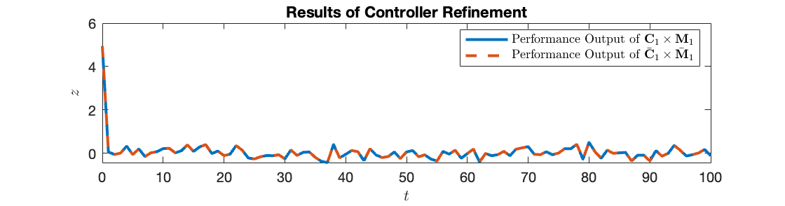
The above example illustrates that the proposed abstraction procedure yields a simplified system in regard to the noise and the controller refinement algorithm will produce a correct-by-design controller for the original model. Even though we considered a simple specification in this example, these results remain unaltered for more complex properties. Similarly, a trivial control design was used in this example, but should any other correct-by-design controller on the abstract model be used, these results remain again unaltered.
Model Reduction with respect to the State. We now investigate model reduction with respect to the state.
Example 2 (continued from Ex. 1)
Assume , a stabilizing solution to (10). Inspired by Lemma 3, consider the abstract model
where and . Due to its structure, system can be reduced to
where and . Utilizing the lower dimensional system , we obtain the correct-by-design controller , after which we use Algorithm 1 to obtain controller . ∎
It is important to note that the above reduction cannot be quantified by existing simulation relations such as [12, 14, 17]. This makes our method a promising new model reduction technique, but for which further research is still necessary. Notice that in Algorithm 1, a minor modification needs to be made based on the obtained reduced model. For instance, in the above example, one must remove the first element of before feeding the remainder to .
Lack of Completeness. The proposed framework is not complete. Due to our choice of knowledge filtering, the original problem might become oversimplified to such a degree that no correct-by-design controller can be obtained for the abstract model. However, this failure to design a controller using the abstract model does not imply that the specification cannot be enforced on the original dynamics.
Example 3 (continued from Ex. 1)
Consider again the linear time-invariant stochastic system (13) with constraint . Consider now matrices , which leads to the following abstract model
where and .
For , no controller exist such that , since maximizing the probability satisfaction of the specification leads to the controller , resulting in . Using the cumulative distribution function again, we can numerically compute that . This means no controller for can enforce specification . However, previously, we have shown how to enforce this specification for a more complex abstract model. Hence, examples 1 and 3 clearly illustrate that while both abstract models simplify the stochastic control synthesis problem, oversimplification may prevent us from finding an adequate controller. ∎
VI Conclusion
In this paper, we proposed a model reduction technique on the noise disturbance, whereby a simpler representation of the original dynamics is obtained by means of reducing state information, which we called knowledge filtering, and via optimal Kalman filtering. We introduce the abstraction procedure, which, under some technical conditions, may lead to a time-invariant abstract model. Our controller refinement algorithm is constructive and allows for the design of correct-by-design controllers on the original dynamics via correct-by-design controllers on the abstract model. We finished the paper by illustrating the abstraction procedure and the controller refinement, by showing how our reduction method can achieve model reduction on the state space, which existing methods, such as those employing simulation relations, cannot realize, and by examining the completeness of our technique.
References
- [1] B. D. Anderson and J. B. Moore, Optimal filtering. Courier Corporation, 2012.
- [2] A. C. Antoulas, Approximation of large-scale dynamical systems. SIAM, 2005.
- [3] C. Baier and J.-P. Katoen, Principles of model checking. MIT press, 2008.
- [4] C. Belta, B. Yordanov, and E. Gol, Formal methods for discrete-time dynamical systems. Springer, 2017, vol. 15.
- [5] D. Bertsekas and S. E. Shreve, Stochastic optimal control: the discrete-time case. Athena Scientific, 1996, vol. 5.
- [6] S. Brechtel, T. Gindele, and R. Dillmann, “Probabilistic decision-making under uncertainty for autonomous driving using continuous POMDPs,” in 17th international IEEE conference on intelligent transportation systems (ITSC), 2014, pp. 392–399.
- [7] N. Cauchi and A. Abate, “ : Automated verification and synthesis of stochastic processes,” in Tools and Algorithms for the Construction and Analysis of Systems, 2019, pp. 247–264.
- [8] A. Donzé, “On signal temporal logic,” in Runtime Verification: 4th International Conference, RV 2013, Rennes, France, September 24-27, 2013. Proceedings 4. Springer, 2013, pp. 382–383.
- [9] A. Girard and G. J. Pappas, “Hierarchical control system design using approximate simulation,” Automatica, vol. 45, pp. 566–571, 2009.
- [10] S. Gugercin, A. C. Antoulas, and C. Beattie, “H_2 model reduction for large-scale linear dynamical systems,” SIAM journal on matrix analysis and applications, vol. 30, no. 2, pp. 609–638, 2008.
- [11] S. Haesaert, N. Cauchi, and A. Abate, “Certified policy synthesis for general markov decision processes,” Performance Evaluation, vol. 117, pp. 75–103, 2017.
- [12] S. Haesaert, S. E. Z. Soudjani, and A. Abate, “Verification of general markov decision processes by approximate similarity relations and policy refinement,” SIAM Journal on Control and Optimization, vol. 55, no. 4, pp. 2333–2367, 2017.
- [13] V. Ionescu and M. Weiss, “Continuous and discrete-time riccati theory: a popov-function approach,” Linear Algebra and its Applications, vol. 193, pp. 173–209, 1993.
- [14] A. A. Julius and G. J. Pappas, “Approximations of stochastic hybrid systems,” IEEE TAC, vol. 54, no. 6, pp. 1193–1203, 2009.
- [15] V. Krishnamurthy, Partially observed Markov decision processes. Cambridge university press, 2016.
- [16] A. Lavaei, M. Khaled, S. Soudjani, and M. Zamani, “Amytiss: Parallelized automated controller synthesis for large-scale stochastic systems,” in International Conference on Computer Aided Verification. Springer, 2020, pp. 461–474.
- [17] G. Pola, C. Manes, A. J. van der Schaft, and M. D. Di Benedetto, “Bisimulation equivalence of discrete-time stochastic linear control systems,” IEEE TAC, vol. 63, no. 7, pp. 1897–1912, 2017.
- [18] R. V. Polyuga and A. Van der Schaft, “Structure preserving model reduction of port-hamiltonian systems by moment matching at infinity,” Automatica, vol. 46, no. 4, pp. 665–672, 2010.
- [19] S. E. Z. Soudjani, C. Gevaerts, and A. Abate, “FAUST2: Formal abstractions of uncountable-state stochastic processes,” in Tools and Algorithms for the Construction and Analysis of Systems. Springer Berlin Heidelberg, 2015, pp. 272–286.
- [20] S. Thrun, “Probabilistic robotics,” Communications of the ACM, vol. 45, no. 3, pp. 52–57, 2002.
- [21] B. Van Huijgevoort, O. Schön, S. Soudjani, and S. Haesaert, “SySCoRe: Synthesis via stochastic coupling relations,” in Proceedings of the 26th ACM International Conference on Hybrid Systems: Computation and Control, 2023, pp. 1–11.
- [22] J. H. van Schuppen, Control and System Theory of Discrete-Time Stochastic Systems. Springer, 2021.
- [23] M. Zamani, P. M. Esfahani, R. Majumdar, A. Abate, and J. Lygeros, “Symbolic control of stochastic systems via approximately bisimilar finite abstractions,” IEEE TAC, vol. 59, no. 12, pp. 3135–3150, 2014.
- [24] M. Zamani, I. Tkachev, and A. Abate, “Towards scalable synthesis of stochastic control systems,” Discrete Event Dynamic Systems, vol. 27, pp. 341–369, 2017.
Appendix
The innovation processes are obtained by simple substitution of the equations (4) and the innovation (5). This is trivial in the case of the a priori innovation process. For the a posteriori innovation process, two additional details will be given. The initial state distribution is obtained from (4a), , and , resulting in . Calculating mean and variance while also noticing that is Gaussian, results in the Gaussian distribution of . The observation output is obtained from substituting (4a) into (5) resulting in . Since , it follows that . Alternatively, notice that contains information about the measured output . Intuitively it makes sense that if the original measurement is used to calculate the expected observation output, the expected observation output will be equivalent to the original measurement.
Lemma 6 (Theorem 1)
and have the same performance output distribution and when given the same input sequence.
Proof:
The proof follows in 3 steps.
Step 1: and have identical performance output distributions when given the same input sequence. This follows directly from .
Step 2: and have the same performance output distributions and when given the same input sequence. To prove this statement, consider the proof of [22, Prop 8.4.3]. There are three differences between [22, Prop 8.4.3] and the setting in this paper, them being the additional input and output in and , and the absence of output noise in . The former two, however, do not influence the result, as can be observed from comparing [22, Theorem 8.3.2 & Theorem 14.4.2] with the former being the main contributor to the proof of [22, Prop 8.4.3]. On the other hand, the exclusion of output noise in is already resolved by the assumption that and .
Step 3: and have the same performance output distributions and when given the same input sequence. Since the innovation processes can be obtained from one another by direct substitution of the Kalman filter equations (4) and the innovation (5), without changing their performance outputs, both have the same performance outputs and when given the same input sequence.
These steps together prove the lemma. ∎
Additional information on the derivation of .
To obtain abstract model , we need to calculate the a posteriori innovation process while assuming an additional measurement is taken at time . To accomplish this, we first calculate the a posteriori state estimate and the a posteriori state variance , to afterwards compute the a posteriori innovation process by utilizing the Kalman filter equations (4), excluding (4f).
Remember , and with and . To compute both a posteriori quantities of , we utilize the following proposition derived from [1, Section 3.1].
Proposition 7
If and are jointly Gaussian, with possessing mean and covariance
then X, conditioned on the information that , is Gaussian, with mean and variance
Utilizing the above proposition, we first calculate the following quantities
Utilizing the Woodbury matrix identity, we identify that
are all equivalent. Let and notice that and . We can now directly compute and , again by utilizing the above proposition. The result is given by
| (14a) | ||||
| (14b) | ||||
Notice that and , the latter of which implies that the a posteriori innovation process will be time-invariant. The a posteriori innovation process can now be obtained from the Kalman filter equations (4), excluding (4f).