DynamicDet: A Unified Dynamic Architecture for Object Detection
Abstract
Dynamic neural network is an emerging research topic in deep learning. With adaptive inference, dynamic models can achieve remarkable accuracy and computational efficiency. However, it is challenging to design a powerful dynamic detector, because of no suitable dynamic architecture and exiting criterion for object detection. To tackle these difficulties, we propose a dynamic framework for object detection, named DynamicDet. Firstly, we carefully design a dynamic architecture based on the nature of the object detection task. Then, we propose an adaptive router to analyze the multi-scale information and to decide the inference route automatically. We also present a novel optimization strategy with an exiting criterion based on the detection losses for our dynamic detectors. Last, we present a variable-speed inference strategy, which helps to realize a wide range of accuracy-speed trade-offs with only one dynamic detector. Extensive experiments conducted on the COCO benchmark demonstrate that the proposed DynamicDet achieves new state-of-the-art accuracy-speed trade-offs. For instance, with comparable accuracy, the inference speed of our dynamic detector Dy-YOLOv7-W6 surpasses YOLOv7-E6 by 12%, YOLOv7-D6 by 17%, and YOLOv7-E6E by 39%. The code is available at https://github.com/VDIGPKU/DynamicDet.

1 Introduction
Object detection is an essential topic in computer vision, as it is a fundamental component for other vision tasks, e.g., autonomous driving shi2020pv; yang20203dssd; liang2022bevfusion, multi-object tracking xu2019spatial; zhang2022bytetrack, intelligent transportation qiu2021deep; yang2022multifeature, etc. In recent years, tremendous progress has been made toward more accurate and faster detectors, such as Network Architecture Search (NAS)-based detectors ghiasi2019fpn; liang2021opanas; wang2022eautodet and YOLO series models bochkovskiy2020yolov4; wang2021scaled; 2022githubyolov5; ge2021yolox; li2022yolov6; wang2022yolov7. However, these methods need to design and train multiple models to achieve a few good trade-offs between accuracy and speed, which is not flexible enough for various application scenarios. To alleviate this problem, we focus on dynamic inference for the object detection task, and attempt to use only one dynamic detector to achieve a wide range of good accuracy-speed trade-offs, as shown in Fig. 1.
The human brain inspires many fields of deep learning, and the dynamic neural network han2021dynamic is a typical one. As two examples shown in Fig. 2, we can quickly identify all objects on the left “easy” image, while we need more time to achieve the same effect for the right one. In other words, the processing speeds of images are different in our brains hubel1962receptive; murata2000selectivity, which depend on the difficulties of the images. This property motivates the image-wise dynamic neural network, and many exciting works have been proposed (e.g., Branchynet teerapittayanon2016branchynet, MSDNet huang2018multiscale, DVT wang2021not). Although these approaches have achieved remarkable performance, they are all designed specifically for the image classification task and are not suitable for other vision tasks, especially for the object detection han2021dynamic. The main difficulties in designing an image-wise dynamic detector are as follows.
Dynamic detectors cannot utilize the existing dynamic architectures. Most existing dynamic architectures are cascaded with multiple stages (i.e., a stack of multiple layers) mcgill2017deciding; huang2018multiscale; jie2019anytime; yang2020resolution, and predict whether to stop the inference at each exiting point. Such a paradigm is feasible in image classification but is ineffective in object detection, since an image has multiple objects and each object usually has different categories and scales, as shown in Fig. 2. Hence, almost all detectors depend heavily on multi-scale information, utilizing the features on different scales to detect objects of different sizes (which are obtained by fusing the multi-scale features of the backbone with a detection neck, i.e., FPN lin2017feature). In this case, the exiting points for detectors can only be placed behind the last stage. Consequently, the entire backbone module has to be run completely zhou2017adaptive, and it is impossible to achieve dynamic inference on multiple cascaded stages.
Dynamic detectors cannot exploit the existing exiting criteria for image classification. For the image classification task, the threshold of top-1 accuracy is a widely used criterion for decision-making huang2018multiscale; wang2021not. Notably, it only needs one fully connected layer to predict the top-1 accuracy at intermediate layer, which is easy and costless. However, object detection task requires the neck and the head to predict the categories and locations of the object instances lin2017feature; ren2015faster; he2017mask; cai2018cascade. Hence, the existing exiting criteria for image classification is not suitable for object detection.
To deal with the above difficulties, we propose a dynamic framework to achieve dynamic inference for object detection, named DynamicDet. Firstly, We design a dynamic architecture for the object detection task, which can exit with multi-scale information during the inference. Then, we propose an adaptive router to choose the best route for each image automatically. Besides, we present the corresponding optimization and inference strategies for the proposed DynamicDet.
Our main contributions are as follows:
- •
We propose a dynamic architecture for object detection, named DynamicDet, which consists of two cascaded detectors and a router. This dynamic architecture can be easily adapted to mainstream detectors, e.g., Faster R-CNN and YOLO.
- •
We propose an adaptive router to predict the difficulty scores of the images based on the multi-scale features, and achieve automatic decision-making. In addition, we propose a hyperparameter-free optimization strategy and a variable-speed inference strategy for our dynamic architecture.
- •
Extensive experiments show that DynamicDet can obtain a wide range of accuracy-speed trade-offs with only one dynamic detector. We also achieve new state-of-the-art trade-offs for real-time object detection (i.e., 56.8% AP at 46 FPS).
2 Related work
2.1 Backbone design on object detection
Backbones play a crucial role in object detectors since the performance of detectors highly relies on the multi-scale features extracted by the backbones chen2019detnas. ResNet he2016deep and its variants (e.g., ResNeXt xie2017aggregated, Res2Net gao2019res2net) introduce the residual connection to neural networks, providing a high-quality backbone architecture family for all vision tasks. Further, to reduce the calculation load, CSPNet wang2020cspnet cuts down the duplicate gradient information to reduce the heavy inference, improving the efficiency significantly. Its effective architecture also inspires many lightweight detectors (e.g., YOLO series models bochkovskiy2020yolov4; wang2021scaled; 2022githubyolov5; ge2021yolox; li2022yolov6; wang2022yolov7). Then, some transformer-based backbones (e.g., PVT wang2021pyramid, Swin Transformer liu2021swin) are proposed to learn the global information better. In addition, many auto-designed backbones chen2019detnas; jiang2020sp; du2020spinenet; sun2022mae for object detection are proposed. For example, DetNAS chen2019detnas utilizes the one-shot supernet to search the optimal backbone, with the guidance of the object detection task.
Although many kinds of backbones have been proposed, almost all of them are single-pass architectures, which sequentially produce one set of multi-scale features. Thus, all stages of them cannot be skipped. Fortunately, some works propose the architectures of multiple cascaded backbones, which have the potential to be converted as a dynamic backbone for object detection. For example, CBNet liu2020cbnet; liang2022cbnet groups multiple identical backbones with composite connections, constructing a more powerful composite backbone. Since these backbones have multiple sub-backbones and each of them can produce intermediate multi-scale features, we can add some exiting points after each sub-backbone for dynamic inference.
2.2 Accuracy-speed trade-off on object detection
Almost all detection methods are designed for a better accuracy-speed trade-off, i.e., more accurate and faster. With a given detector, the simplest way to obtain an accuracy-speed trade-off is to adopt the model scaling techniques tan2020efficientdet; wang2021scaled; wang2022yolov7 (e.g., increasing the channel size or repeating the layers). EfficientDet tan2020efficientdet uniformly scales the resolution, depth, and width for all modules simultaneously, achieving remarkable efficiency on real-time detectors. Scaled-YOLOv4 wang2021scaled modifies not only the depth, width, and resolution but also the structure of the network to pursue a better trade-off. YOLOv7 wang2022yolov7 designs a compound scaling method for concatenation-based models, achieving new state-of-the-art trade-offs. EAutoDet wang2022eautodet constructs a supernet and adopts Network Architecture Search (NAS) to automatically search for suitable scaling factors under different hardware constraints. However, all the above methods need to train multiple detectors for the best trade-offs (e.g., one tiny model for real-time detection and another large model for accurate detection), leading to colossal training resources. In this paper, we focus on dynamic inference, aiming to achieve a wide range of best accuracy-speed trade-offs with only one dynamic detector.
2.3 Dynamic neural network
The dynamic neural network can achieve adaptive computation for different images (i.e., image-wise teerapittayanon2016branchynet; wang2018skipnet; huang2018multiscale; li2019improved; jie2019anytime; yang2020resolution; wang2021not; li2021dynamic) or pixels (i.e., spatial-wise figurnov2017spatially; rao2021dynamicvit; han2022latency). SACT figurnov2017spatially is a classic spatial-wise dynamic network, which adaptively adjusts the number of executed layers for the regions of the image, to improve the efficiency of networks. Its practical speed-up performance highly relies on the hardware-software co-design han2021dynamic. However, the current deep learning hardware and libraries abadi2016tensorflow; paszke2019pytorch are not friendly to these spatial-wise dynamic networks han2021dynamic. On the contrary, image-wise dynamic networks do not rely on sparse computing and can be easily accelerated on the conventional CPUs and GPUs choquette2021nvidia. Branchynet teerapittayanon2016branchynet introduces the early exiting strategy, which enables the model to exit from the intermediate layer whenever the model is confident enough. MSDNet huang2018multiscale and its variants li2019improved; yang2020resolution develop a multi-classifier architecture for the image classification task. DVT wang2021not cascades multiple transformers with increasing numbers of tokens and activates them sequentially to achieve dynamic inference. However, these methods are all designed specifically for the image classification task and cannot be applied to other vision tasks, such as object detection.
The closest work to our DynamicDet is Adaptive Feeding zhou2017adaptive. In Adaptive Feeding zhou2017adaptive, each image is detected by a lightweight detector (e.g., Tiny YOLO redmon2016you) and then classified as easy or hard by a linear support vector machine (SVM) with those detected results. Then, the easy images will go through a fast detector (e.g., SSD300 liu2016ssd), while the hard images will go through a more accurate but slower one (e.g., SSD500 liu2016ssd). Adaptive Feeding zhou2017adaptive introduces the above multi-stage process for dynamic inference, which is inefficient and not elegant. In comparison, the proposed DynamicDet cascades two detectors and a classifier (i.e., the router), yielding a more unified and efficient dynamic detector.
3 Approach
In the following, we elaborate on our dynamic architecture for object detection. We first introduce the overall architecture in Section 3.1. Then, we state the proposed adaptive router, i.e., the decision maker of DynamicDet in Section 3.2. Finally, we introduce the optimization strategy and a variable-speed inference strategy in Sections 3.3 and 3.4.
3.1 Overall architecture
The overall architecture of our dynamic detector is shown in Fig. 3. Inspired by CBNet liu2020cbnet; liang2022cbnet, our dynamic architecture consists of two detectors and one router. For an input image , we initially extract its multi-scale features with the first backbone as
| (1) |
where denotes the number of stages, i.e., the number of multi-scale features. Then, the router will be fed with these features to predict a difficulty score for this image as
| (2) |
Generally speaking, the “easy” images exit at the first backbone, while the “hard” images require the further processing. Specifically, if the router classifies the input image as an “easy” one, the followed neck and head will output the detection results as
| (3) |
On the contrary, if the router classifies the input image as a “hard” one, the multi-scale features will need further enhancement by the second backbone, instead of immediately decoded by . In particular, we embed the multi-scale features into by a composite connection module as
| (4) |
where is the DHLC of CBNet liu2020cbnet; liang2022cbnet in our implementation. Then, we feed the input image into the second backbone and enhance the features of the second backbone via summing the corresponding elements of at each stage sequentially, denoted as
| (5) |
and the detection results will be obtained by the second head and neck as
| (6) |
Through the above process, the “easy” images will be processed by only one backbone, while the “hard” images will be processed by two. Obviously, with such an architecture, trades-offs between computation (i.e., speed) and accuracy can be achieved.
3.2 Adaptive router
In mainstream object detectors, different scale features play different roles. Generally, the features of the shallow layers, with strong spatial information and small receptive fields, are more used to detect small objects. In contrast, the features of the deep layers, with strong semantic information and large receptive fields, are more used to detect large objects. This property makes it necessary to consider multi-scale information when predicting the difficulty score of an image. According to this, we design an adaptive router based on the multi-scale features, that is, a simple yet effective decision-maker for the dynamic detector.
Inspired by the squeeze-and-excitation (SE) module hu2018squeeze, we first pool the multi-scale features independently and concatenate them all as
| (7) |
where denotes the global average pooling and denotes the channel-wise concatenation. With this operation, we compress the multi-scale features into a vector of dimension . Then, we map this vector to a difficulty score via two learnable fully connected layers as
| (8) |
where denote the ReLU and Sigmoid activation functions respectively, and are learnable parameters. Following zhu2020dynamic, we reduce the feature dimension to in the first fully connected layer, and exploit the second fully connected layer with a Sigmoid function to generate the predicted score. It is worth noting that the computational burden of our router can be negligible since we first pool all multi-scale features to one vector.

3.3 Optimization strategy
In this section, we describe the optimization strategy for the above dynamic architecture.
Firstly, we jointly train the cascaded detectors, and the training objective is
| (9) |
where denote the input image and the ground truth respectively, denotes the learnable parameters of the detector and denotes the training loss for detector (e.g., bounding box regression loss and classification loss). After the above training phase, these two detectors will be able to detect the objects, and we freeze their parameters during the later training.
Then, we train the adaptive router to automatically distinguish the difficulty of the image. Here, we assume the parameters of the router are and the predicted difficulty score obtained from the Eq. 8 is . We hope the router can assign the “easy” images (i.e., with lower ) to the faster detector (i.e., the first detector) and the “hard” images (i.e., with higher ) to the more accurate detector (i.e., the second detector).
However, it is non-trivial to implement that in practice. If we directly optimize the router without any constraints as
| (10) | ||||
the router will always choose the most accurate detector as it allows for a lower training loss. Furthermore, if we naively add hardware constraints to the training objective as
| (11) | ||||
we will have to adjust the hyperparameter by try and error, leading to huge workforce consumption.
To overcome the above challenges, we propose a hyperparameter-free optimization strategy for our adaptive router. First, we define the difficulty criterion based on the corresponding training loss difference between two detectors of an image, as shown in Fig. 4. Specifically, we assume that if the loss difference of an image between two detectors is small enough, this image can be classified as an “easy” image. Instead, if the loss difference is large enough, it should be classified as a “hard” image. Ideally, for a balanced situation, we hope the easier half of all images go through the first detector, and the harder half go through the second one. To achieve this, we introduce an adaptive offset to balance the losses of two detectors and optimize our router via gradient descent. In practice, we first calculate the median of the training loss difference between the first and the second detector on the training set. Then, the training objective of our router can be formulated as
| (12) | ||||
where is used to reward the first detector and punish the second detector, respectively. As the qualitative analysis shown in Fig. 5, without this reward and penalty, the losses of the second detector are always smaller than the first detector. When the reward and penalty are conducted, their loss curves intersect and reveal the optimal curve.
Our training objective provides a means to optimize the adaptive router by introducing the following gradient through the difficulty score to all parameters of the router as
| (13) |
To distinguish between “easy” and “hard” images better, we expect the optimization direction of the router to be related to the difficulty of the image, i.e., the difference in loss between the two detectors. Obviously, the gradient at Eq. 13 enable such expectation.
| Model | Size | FLOPs | FPS | AP |
| EAutoDet-X wang2022eautodet | 640 | 225.3G | 41† | 49.2 |
| YOLOX-L ge2021yolox | 640 | 155.6G | 69† | 50.1 |
| YOLOX-X ge2021yolox | 640 | 281.9G | 58† | 51.5 |
| YOLOv5-L (r6.2) 2022githubyolov5 | 640 | 109.1G | 114 | 49.0 |
| YOLOv5-X (r6.2) 2022githubyolov5 | 640 | 205.7G | 100 | 50.9 |
| YOLOv6-M li2022yolov6 | 640 | 82.2G | 109 | 49.6 |
| YOLOv6-L li2022yolov6 | 640 | 144.0G | 76 | 52.4 |
| PP-YOLOE+-M xu2022pp | 640 | 49.9G | 123† | 50.0 |
| PP-YOLOE+-L xu2022pp | 640 | 110.1G | 78† | 53.3 |
| PP-YOLOE+-X xu2022pp | 640 | 206.6G | 45† | 54.9 |
| YOLOv7 wang2022yolov7 | 640 | 104.7G | 114 | 51.4 |
| Dy-YOLOv7 / 10 | 640 | 112.4G | 110 | 52.1 |
| Dy-YOLOv7 / 50 | 640 | 143.2G | 96 | 53.3 |
| Dy-YOLOv7 / 90 | 640 | 174.0G | 85 | 53.8 |
| Dy-YOLOv7 / 100 | 640 | 181.7G | 83 | 53.9 |
| YOLOv7-X wang2022yolov7 | 640 | 189.9G | 105 | 53.1 |
| Dy-YOLOv7-X / 10 | 640 | 201.7G | 98 | 53.3 |
| Dy-YOLOv7-X / 50 | 640 | 248.9G | 78 | 54.4 |
| Dy-YOLOv7-X / 90 | 640 | 296.1G | 65 | 55.0 |
| Dy-YOLOv7-X / 100 | 640 | 307.9G | 64 | 55.0 |
| YOLOv5-M6 (r6.2) 2022githubyolov5 | 1280 | 200.0G | 96 | 51.4 |
| YOLOv5-L6 (r6.2) 2022githubyolov5 | 1280 | 445.6G | 65 | 53.8 |
| YOLOv5-X6 (r6.2) 2022githubyolov5 | 1280 | 839.2G | 39 | 55.0 |
| YOLOv7-W6 wang2022yolov7 | 1280 | 360.0G | 78 | 54.9 |
| YOLOv7-E6 wang2022yolov7 | 1280 | 515.2G | 52 | 56.0 |
| YOLOv7-D6 wang2022yolov7 | 1280 | 806.8G | 41 | 56.6 |
| YOLOv7-E6E wang2022yolov7 | 1280 | 843.2G | 33 | 56.8 |
| Dy-YOLOv7-W6 / 10 | 1280 | 384.2G | 74 | 55.2 |
| Dy-YOLOv7-W6 / 50 | 1280 | 480.8G | 58 | 56.1 |
| Dy-YOLOv7-W6 / 90 | 1280 | 577.4G | 48 | 56.7 |
| Dy-YOLOv7-W6 / 100 | 1280 | 601.6G | 46 | 56.8 |
- 1
The FPS marked with are from the corresponding papers, and others are measured on the same machine with 1 NVIDIA V100 GPU.
3.4 Variable-speed inference
We further propose a simple and effective method to determine the difficulty score thresholds to achieve variable-speed inference with only one dynamic detector. Specifically, our adaptive router will output a difficulty score and decide which detector to go through based on a certain threshold during inference. Therefore, we can set different thresholds to achieve different accuracy-speed trade-offs. Firstly, we count the difficulty scores of the validation set. Then, based on the actual needs (e.g., the target latency), we can obtain the corresponding threshold for our router. For example, assuming the latency of the first detector is , the latency of the cascaded two detectors is and the target latency is , we can calculate the maximum allowable proportion of the “hard” images as
| (14) |
and then the threshold will be
| (15) |
where means to compute the -th quantile of the data. It is worth noting that this threshold is robust in both validation set and test set because these two sets are independent and identically distributed (i.e., i.i.d.).
Based on the above strategy, one dynamic detector can directly cover the accuracy-speed trade-offs from the single to double detectors, avoiding redesigning and training multiple detectors under different hardware constraints.
4 Experiments
In this section, we evaluate our DynamicDet through extensive experiments. In Section 4.1, we detail the experimental setups. In Section 4.2, we compare our DynamicDet with the state-of-the-art real-time detectors. In Section 4.3, we present the experimental results on two-stage detectors with CNN- and transformer-based backbones to demonstrate the generality of DynamicDet over different backbones and detectors. In Section 4.4, we ablate each component of DynamicDet in detail. In Section 4.5, we visualize the “easy” and the “hard” images determined by the adaptive router.
4.1 Experimental setups
We conduct experiments on the COCO lin2014microsoft benchmark. All the models presented are trained on the 118k training images, and tested on the 5k minival images and 20k test-dev images. We choose the YOLOv7 wang2022yolov7 series models as the real-time detector baseline, and the Faster R-CNN ren2015faster (ResNet he2016deep) and the Mask R-CNN he2017mask (Swin Transformer liu2021swin) as the two-stage detector baselines. All dynamic detectors are trained with the same hyper-parameters of their corresponding baselines. We use brief notation to indicate the easy-hard proportion for each dynamic detector: for instance, “Dy-YOLOv7-X/10” means the dynamic YOLOv7-X model with 10% images are classified as “hard” and the rest are classified as “easy”. The training of the adaptive router is conducted on a single GPU with batchsize 1 and two epochs, utilizing the AdamW loshchilov2017decoupled optimizer with a constant learning rate and weight decay . The reported FLOPs for dynamic detectors are the average FLOPs on the corresponding dataset. The speed performance is measured on a machine with 1 NVIDIA V100 GPU unless otherwise stated. The implementation of Dy-YOLOv7 is developed by the YOLOv7 wang2022yolov7 framework, with two identical detectors. The implementation of dynamic two-stage detectors is developed by the open-source CBNet liang2022cbnet framework, with two identical backbones and a shared neck and head.
4.2 Comparison with the state-of-the-arts
As shown in Table 1, compared with the state-of-the-art high-performance real-time object detectors, our dynamic detectors obtain better results and achieve the new state-of-the-art accuracy-speed trade-offs. Specifically, Dy-YOLOv7-W6 / 50 achieves 56.1% AP with 58 FPS, which is 0.1% more accurate and 12% faster than YOLOv7-E6. Dy-YOLOv7-W6 / 100 achieves 56.8% AP with 46 FPS, which is 39% faster than YOLOv7-E6E with a similar accuracy. It is worth noting that these trade-offs are obtained by only one dynamic detector instead of multiple independent models.
4.3 Generality for two-stage detectors
| Model | FLOPs | FPS | AP | AP |
| Faster R-CNN ResNet50 ren2015faster; he2016deep | 207.1G | 23 | 37.4 | - |
| Faster R-CNN ResNet101 ren2015faster; he2016deep | 283.1G | 18 | 39.4 | - |
| Dy-Faster R-CNN ResNet50 / 50 | 245.4G | 20 | 39.5 | - |
| Dy-Faster R-CNN ResNet50 / 90 | 276.0G | 17 | 40.4 | - |
| Mask R-CNN Swin-T he2017mask; liu2021swin | 263.8G | 15 | 46.0 | 41.6 |
| Mask R-CNN Swin-S he2017mask; liu2021swin | 353.8G | 12 | 48.2 | 43.2 |
| Dy-Mask R-CNN Swin-T / 50 | 310.6G | 12 | 48.7 | 43.6 |
| Dy-Mask R-CNN Swin-T / 90 | 348.0G | 11 | 49.9 | 44.2 |
We conduct experiments on two classic two-stage detectors (i.e., Faster R-CNN ren2015faster, Mask R-CNN he2017mask) to show the generality of our DynamicDet. As shown in Table 2, our method is compatible with two-stage detectors and can also improve the accuracy-speed performance of baselines. For example, Dy-Faster R-CNN ResNet50 / 90 boosts the bbox AP by 1% with the comparable inference speed for Faster R-CNN ResNet101. Furthermore, DynamicDet is also compatible with transformer-based backbones (e.g., Swin Transformer liu2021swin). Dy-Mask R-CNN Swin-T / 90 improves the bbox AP to 49.9% with the comparable inference speed of Mask R-CNN Swin-S. Notably, our two-stage dynamic detector can also perform variable-speed inference as illustrated in Fig. 6.
4.4 Ablation study
4.4.1 Lightweight adaptive router
The FLOPs ratios for the adaptive router in different models are presented in Table 3. We can find that this ratio is less than 0.002% in all models, demonstrating that the computational burden of the adaptive router can be negligible. This lightweight router avoids slowing down the detection process and ensures the fast decision-making for dynamic inference.
4.4.2 Effective training strategy for adaptive router
We ablate the effectiveness of the proposed training and optimization strategy for adaptive router. We first train a Mask R-CNN he2017mask with cascaded Swin-T liu2021swin as our baseline detector. Then, we apply three strategies to achieve the decision-making for router: random, AP-based (i.e., dividing “easy” and “hard” images based on the validation accuracy and using them to train the router, similar to Adaptive Feeding zhou2017adaptive), and our proposed strategy. As shown in Fig. 7, we compare the bbox AP on the test-dev set of different training strategies. It is shown that our optimization strategy outperforms another two strategies under all latency constraints. Taking the detector with 84.5 ms latency (i.e., 50% easy and 50% hard) as an example, our strategy exceeds random selection 0.9% AP and AP-based strategy 0.7% AP. This proves that our optimization strategy effectively improves the discrimination accuracy of the router and outperforms AP-based strategy zhou2017adaptive.
| Model | Router | Total | Ratio |
| Dy-YOLOv7 | 2.1M | 104.7G | 0.0020% |
| Dy-YOLOv7-W6 | 1.9M | 360.0G | 0.0005% |
| Dy-Faster R-CNN ResNet50 | 3.7M | 283.7G | 0.0013% |
| Dy-Mask R-CNN Swin-T | 0.5M | 357.4G | 0.0001% |
4.4.3 Robust variable-speed inference strategy
To achieve variable-speed inference for a dynamic detector, we count the difficulty scores on the validation set and directly adopt the corresponding thresholds for the test set. This strategy requires the validation set to be large enough. However, with custom datasets, this is not always sufficient. To demonstrate the robustness of our variable-speed inference strategy, we analyze the impact of the validation set size on the threshold consistency between the validation set and test set. Taking the Dy-Mask R-CNN Swin-T on COCO lin2014microsoft dataset as an example, its threshold for 50% quantile on the test set is 0.62. Then, we count the thresholds for 50% quantile on the validation set of different sizes (i.e., 0.5k, 1k, , 5k). As shown in Fig. 9, the threshold obtained from 5k validation images is consistent with the threshold of the test set, which confirms our assumption in Section 3.4. Later, as the data size decreases, the thresholds of the validation set change within a small range. However, when the data size is less than 1.5k, the threshold of the validation set and the test set will occur a large deviation (i.e., 0.11 at 1k). Overall, our variable-speed inference strategy is stable when the validation set size is relatively sufficient (e.g., about 2k validation images for the 20k test set on COCO lin2014microsoft).
4.4.4 Comparison with the trade-offs obtained by adjusting the input resolution
For a well-trained detector, changing its input resolution can also quickly obtain a series of accuracy-speed trade-offs. Here we compare this method with our dynamic detector. As shown in Fig. 10, we compare our Dy-YOLOv7-W6 and the YOLOv7-D6 with different input resolutions (i.e., 6401280), and we observe that our dynamic detector achieves better accuracy-speed trade-offs. For example, our Dy-YOLOv7-W6 achieves 55.2% AP at 74 FPS (13.5 ms), while YOLOv7-D6 with 640 input resolution only achieves 52.2% AP at an even slower inference speed.
4.5 Visualization of images with different difficulty scores
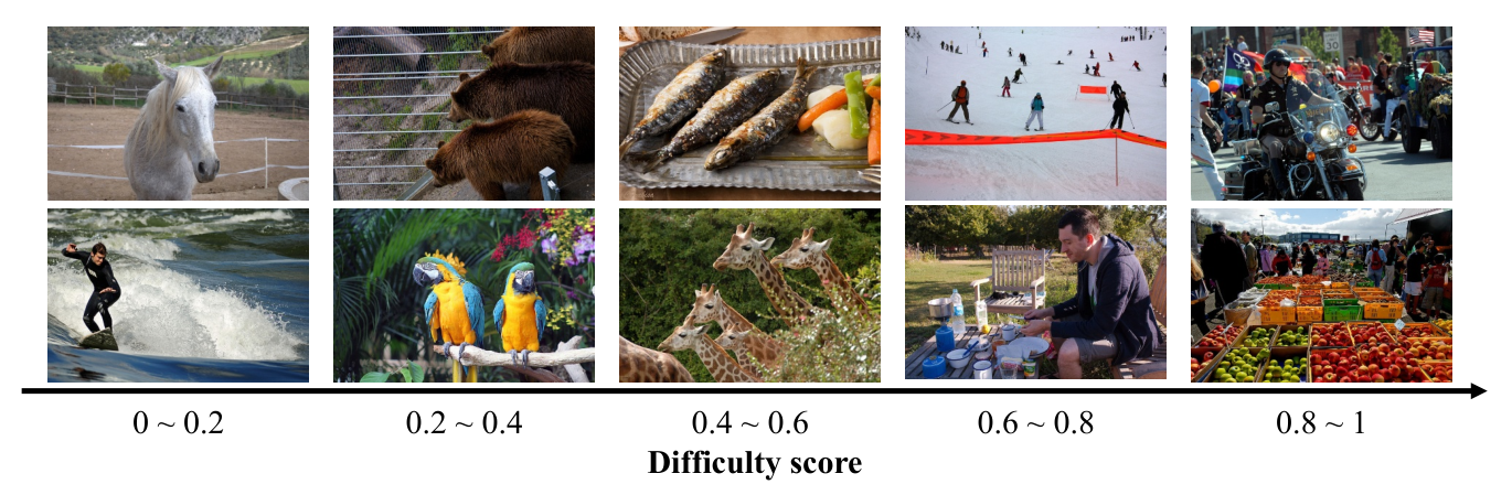
We depict the images with different predicted difficulty scores in Fig. 8, ascending from left to right. That is, the images on the left are considered as the “easy” images, while those on the right are considered as the “hard” images. We can observe that the “easy” images usually contain fewer objects, with the usual camera viewpoint and the clean background. In contrast, the “hard” images usually have more complex scenes with severe occlusion and much more small objects.
5 Conclusion
In this paper, we present a unified dynamic architecture for object detection, DynamicDet. We first design a dynamic architecture to support dynamic inference on mainstream detectors. Then, we propose an adaptive router to predict the difficulty score of each image and determine the inference route. With the above architecture and router, we then propose a hyperparameter-free optimization strategy with an adaptive offset to training our dynamic detectors. Last, we present a variable-speed inference strategy. With the settable threshold for dynamic inference, we can achieve a wide range of accuracy-speed trade-offs with only one dynamic detector. Extensive experimental results demonstrate the superiority of the proposed DynamicDet in accuracy and efficiency, and new state-of-the-art accuracy-speed trade-offs are achieved.
Acknowledgments
This work was supported by National Natural Science Foundation of China under Grant 62176007. This work was also a research achievement of Key Laboratory of Science, Technology and Standard in Press Industry (Key Laboratory of Intelligent Press Media Technology).
References
- (1) Martín Abadi, Paul Barham, Jianmin Chen, Zhifeng Chen, Andy Davis, Jeffrey Dean, Matthieu Devin, Sanjay Ghemawat, Geoffrey Irving, Michael Isard, et al. Tensorflow: a system for large-scale machine learning. In 12th USENIX symposium on operating systems design and implementation (OSDI 16), pages 265–283, 2016.
- (2) Alexey Bochkovskiy, Chien-Yao Wang, and Hong-Yuan Mark Liao. Yolov4: Optimal speed and accuracy of object detection. arXiv preprint arXiv:2004.10934, 2020.
- (3) Zhaowei Cai and Nuno Vasconcelos. Cascade r-cnn: Delving into high quality object detection. In CVPR, pages 6154–6162, 2018.
- (4) Yukang Chen, Tong Yang, Xiangyu Zhang, Gaofeng Meng, Xinyu Xiao, and Jian Sun. Detnas: Backbone search for object detection. NeurIPS, 32, 2019.
- (5) Jack Choquette, Wishwesh Gandhi, Olivier Giroux, Nick Stam, and Ronny Krashinsky. Nvidia a100 tensor core gpu: Performance and innovation. IEEE Micro, 41(2):29–35, 2021.
- (6) Xianzhi Du, Tsung-Yi Lin, Pengchong Jin, Golnaz Ghiasi, Mingxing Tan, Yin Cui, Quoc V Le, and Xiaodan Song. Spinenet: Learning scale-permuted backbone for recognition and localization. In CVPR, pages 11592–11601, 2020.
- (7) Michael Figurnov, Maxwell D Collins, Yukun Zhu, Li Zhang, Jonathan Huang, Dmitry Vetrov, and Ruslan Salakhutdinov. Spatially adaptive computation time for residual networks. In CVPR, pages 1039–1048, 2017.
- (8) Shang-Hua Gao, Ming-Ming Cheng, Kai Zhao, Xin-Yu Zhang, Ming-Hsuan Yang, and Philip Torr. Res2net: A new multi-scale backbone architecture. IEEE TPAMI, 43(2):652–662, 2019.
- (9) Zheng Ge, Songtao Liu, Feng Wang, Zeming Li, and Jian Sun. Yolox: Exceeding yolo series in 2021. arXiv preprint arXiv:2107.08430, 2021.
- (10) Golnaz Ghiasi, Tsung-Yi Lin, and Quoc V Le. Nas-fpn: Learning scalable feature pyramid architecture for object detection. In CVPR, pages 7036–7045, 2019.
- (11) Jocher Glenn. Yolov5 release v6.2, 2022. https://github.com/ultralytics/yolov5/releases/tag/v6.2.
- (12) Yizeng Han, Gao Huang, Shiji Song, Le Yang, Honghui Wang, and Yulin Wang. Dynamic neural networks: A survey. IEEE TPAMI, 2021.
- (13) Yizeng Han, Zhihang Yuan, Yifan Pu, Chenhao Xue, Shiji Song, Guangyu Sun, and Gao Huang. Latency-aware spatial-wise dynamic networks. In NeurIPS, 2022.
- (14) Kaiming He, Georgia Gkioxari, Piotr Dollár, and Ross Girshick. Mask r-cnn. In ICCV, pages 2961–2969, 2017.
- (15) Kaiming He, Xiangyu Zhang, Shaoqing Ren, and Jian Sun. Deep residual learning for image recognition. In CVPR, pages 770–778, 2016.
- (16) Jie Hu, Li Shen, and Gang Sun. Squeeze-and-excitation networks. In CVPR, pages 7132–7141, 2018.
- (17) Gao Huang, Danlu Chen, Tianhong Li, Felix Wu, Laurens van der Maaten, and Kilian Weinberger. Multi-scale dense networks for resource efficient image classification. In ICLR, 2018.
- (18) David H Hubel and Torsten N Wiesel. Receptive fields, binocular interaction and functional architecture in the cat’s visual cortex. The Journal of physiology, 160(1):106, 1962.
- (19) Chenhan Jiang, Hang Xu, Wei Zhang, Xiaodan Liang, and Zhenguo Li. Sp-nas: Serial-to-parallel backbone search for object detection. In CVPR, pages 11863–11872, 2020.
- (20) Zequn Jie, Peng Sun, Xin Li, Jiashi Feng, and Wei Liu. Anytime recognition with routing convolutional networks. IEEE TPAMI, 43(6):1875–1886, 2019.
- (21) Chuyi Li, Lulu Li, Hongliang Jiang, Kaiheng Weng, Yifei Geng, Liang Li, Zaidan Ke, Qingyuan Li, Meng Cheng, Weiqiang Nie, et al. Yolov6: a single-stage object detection framework for industrial applications. arXiv preprint arXiv:2209.02976, 2022.
- (22) Changlin Li, Guangrun Wang, Bing Wang, Xiaodan Liang, Zhihui Li, and Xiaojun Chang. Dynamic slimmable network. In CVPR, pages 8607–8617, 2021.
- (23) Hao Li, Hong Zhang, Xiaojuan Qi, Ruigang Yang, and Gao Huang. Improved techniques for training adaptive deep networks. In ICCV, pages 1891–1900, 2019.
- (24) Tingting Liang, Xiaojie Chu, Yudong Liu, Yongtao Wang, Zhi Tang, Wei Chu, Jingdong Chen, and Haibin Ling. Cbnet: A composite backbone network architecture for object detection. IEEE TIP, 2022.
- (25) Tingting Liang, Yongtao Wang, Zhi Tang, Guosheng Hu, and Haibin Ling. Opanas: One-shot path aggregation network architecture search for object detection. In CVPR, pages 10195–10203, 2021.
- (26) Tingting Liang, Hongwei Xie, Kaicheng Yu, Zhongyu Xia, Zhiwei Lin, Yongtao Wang, Tao Tang, Bing Wang, and Zhi Tang. Bevfusion: A simple and robust lidar-camera fusion framework. In NeurIPS, 2022.
- (27) Tsung-Yi Lin, Piotr Dollár, Ross Girshick, Kaiming He, Bharath Hariharan, and Serge Belongie. Feature pyramid networks for object detection. In CVPR, pages 2117–2125, 2017.
- (28) Tsung-Yi Lin, Michael Maire, Serge Belongie, James Hays, Pietro Perona, Deva Ramanan, Piotr Dollár, and C Lawrence Zitnick. Microsoft coco: Common objects in context. In ECCV, pages 740–755. Springer, 2014.
- (29) Wei Liu, Dragomir Anguelov, Dumitru Erhan, Christian Szegedy, Scott Reed, Cheng-Yang Fu, and Alexander C Berg. Ssd: Single shot multibox detector. In ECCV, pages 21–37. Springer, 2016.
- (30) Yudong Liu, Yongtao Wang, Siwei Wang, TingTing Liang, Qijie Zhao, Zhi Tang, and Haibin Ling. Cbnet: A novel composite backbone network architecture for object detection. In AAAI, volume 34, pages 11653–11660, 2020.
- (31) Ze Liu, Yutong Lin, Yue Cao, Han Hu, Yixuan Wei, Zheng Zhang, Stephen Lin, and Baining Guo. Swin transformer: Hierarchical vision transformer using shifted windows. In ICCV, pages 10012–10022, 2021.
- (32) Ilya Loshchilov and Frank Hutter. Decoupled weight decay regularization. arXiv preprint arXiv:1711.05101, 2017.
- (33) Mason McGill and Pietro Perona. Deciding how to decide: Dynamic routing in artificial neural networks. In International Conference on Machine Learning, pages 2363–2372. PMLR, 2017.
- (34) Akira Murata, Vittorio Gallese, Giuseppe Luppino, Masakazu Kaseda, and Hideo Sakata. Selectivity for the shape, size, and orientation of objects for grasping in neurons of monkey parietal area aip. Journal of neurophysiology, 83(5):2580–2601, 2000.
- (35) Adam Paszke, Sam Gross, Francisco Massa, Adam Lerer, James Bradbury, Gregory Chanan, Trevor Killeen, Zeming Lin, Natalia Gimelshein, Luca Antiga, et al. Pytorch: An imperative style, high-performance deep learning library. NeurIPS, 32, 2019.
- (36) Linrun Qiu, Dongbo Zhang, Yuan Tian, and Najla Al-Nabhan. Deep learning-based algorithm for vehicle detection in intelligent transportation systems. The Journal of Supercomputing, 77(10):11083–11098, 2021.
- (37) Yongming Rao, Wenliang Zhao, Benlin Liu, Jiwen Lu, Jie Zhou, and Cho-Jui Hsieh. Dynamicvit: Efficient vision transformers with dynamic token sparsification. NeurIPS, 34:13937–13949, 2021.
- (38) Joseph Redmon, Santosh Divvala, Ross Girshick, and Ali Farhadi. You only look once: Unified, real-time object detection. In CVPR, pages 779–788, 2016.
- (39) Shaoqing Ren, Kaiming He, Ross Girshick, and Jian Sun. Faster r-cnn: Towards real-time object detection with region proposal networks. NeurIPS, 28, 2015.
- (40) Shaoshuai Shi, Chaoxu Guo, Li Jiang, Zhe Wang, Jianping Shi, Xiaogang Wang, and Hongsheng Li. Pv-rcnn: Point-voxel feature set abstraction for 3d object detection. In CVPR, pages 10529–10538, 2020.
- (41) Zhenhong Sun, Ming Lin, Xiuyu Sun, Zhiyu Tan, Hao Li, and Rong Jin. Mae-det: Revisiting maximum entropy principle in zero-shot nas for efficient object detection. In International Conference on Machine Learning, pages 20810–20826. PMLR, 2022.
- (42) Mingxing Tan, Ruoming Pang, and Quoc V Le. Efficientdet: Scalable and efficient object detection. In CVPR, pages 10781–10790, 2020.
- (43) Surat Teerapittayanon, Bradley McDanel, and Hsiang-Tsung Kung. Branchynet: Fast inference via early exiting from deep neural networks. In ICPR, pages 2464–2469. IEEE, 2016.
- (44) Chien-Yao Wang, Alexey Bochkovskiy, and Hong-Yuan Mark Liao. Scaled-yolov4: Scaling cross stage partial network. In CVPR, pages 13029–13038, 2021.
- (45) Chien-Yao Wang, Alexey Bochkovskiy, and Hong-Yuan Mark Liao. Yolov7: Trainable bag-of-freebies sets new state-of-the-art for real-time object detectors. arXiv preprint arXiv:2207.02696, 2022.
- (46) Chien-Yao Wang, Hong-Yuan Mark Liao, Yueh-Hua Wu, Ping-Yang Chen, Jun-Wei Hsieh, and I-Hau Yeh. Cspnet: A new backbone that can enhance learning capability of cnn. In CVPRW, pages 390–391, 2020.
- (47) Wenhai Wang, Enze Xie, Xiang Li, Deng-Ping Fan, Kaitao Song, Ding Liang, Tong Lu, Ping Luo, and Ling Shao. Pyramid vision transformer: A versatile backbone for dense prediction without convolutions. In ICCV, pages 568–578, 2021.
- (48) Xiaoxing Wang, Jiale Lin, Juanping Zhao, Xiaokang Yang, and Junchi Yan. Eautodet: efficient architecture search for object detection. In ECCV, pages 668–684. Springer, 2022.
- (49) Xin Wang, Fisher Yu, Zi-Yi Dou, Trevor Darrell, and Joseph E Gonzalez. Skipnet: Learning dynamic routing in convolutional networks. In ECCV, pages 409–424, 2018.
- (50) Yulin Wang, Rui Huang, Shiji Song, Zeyi Huang, and Gao Huang. Not all images are worth 16x16 words: Dynamic transformers for efficient image recognition. NeurIPS, 34:11960–11973, 2021.
- (51) Saining Xie, Ross Girshick, Piotr Dollár, Zhuowen Tu, and Kaiming He. Aggregated residual transformations for deep neural networks. In CVPR, pages 1492–1500, 2017.
- (52) Jiarui Xu, Yue Cao, Zheng Zhang, and Han Hu. Spatial-temporal relation networks for multi-object tracking. In ICCV, pages 3988–3998, 2019.
- (53) Shangliang Xu, Xinxin Wang, Wenyu Lv, Qinyao Chang, Cheng Cui, Kaipeng Deng, Guanzhong Wang, Qingqing Dang, Shengyu Wei, Yuning Du, et al. Pp-yoloe: An evolved version of yolo. arXiv preprint arXiv:2203.16250, 2022.
- (54) Le Yang, Yizeng Han, Xi Chen, Shiji Song, Jifeng Dai, and Gao Huang. Resolution adaptive networks for efficient inference. In CVPR, pages 2369–2378, 2020.
- (55) Shuo Yang, Huimin Lu, and Jianru Li. Multifeature fusion-based object detection for intelligent transportation systems. IEEE Transactions on Intelligent Transportation Systems, 2022.
- (56) Zetong Yang, Yanan Sun, Shu Liu, and Jiaya Jia. 3dssd: Point-based 3d single stage object detector. In CVPR, pages 11040–11048, 2020.
- (57) Yifu Zhang, Peize Sun, Yi Jiang, Dongdong Yu, Fucheng Weng, Zehuan Yuan, Ping Luo, Wenyu Liu, and Xinggang Wang. Bytetrack: Multi-object tracking by associating every detection box. In ECCV, pages 1–21. Springer, 2022.
- (58) Hong-Yu Zhou, Bin-Bin Gao, and Jianxin Wu. Adaptive feeding: Achieving fast and accurate detections by adaptively combining object detectors. In CVPR, pages 3505–3513, 2017.
- (59) Mingjian Zhu, Kai Han, Changbin Yu, and Yunhe Wang. Dynamic feature pyramid networks for object detection. arXiv preprint arXiv:2012.00779, 2020.
Appendix A Pseudo code for dynamic detector
We present the pseudo code of training the adaptive router on Algorithm 1, and the dynamic inference on Algorithm 2.
Appendix B Additional results
B.1 More comparison on real-time object detection
We present more precision results (e.g., AP) to compare with other real-time object detectors in Table 4.
B.2 More results for dynamic detectors
We present more results for our dynamic detector (i.e., Dy-YOLOv7 with / 0, / 10, …, / 100) in Table 5. It is observed that our dynamic detectors can obtain a wide range of trade-offs of different precision and speed by proposed variable-speed inference strategy. For instance, using the same weight with different thresholds for inference, our Dy-YOLOv7-W6 can achieve 54.7%56.8% mAP with 7846 FPS.
| Model | Size | FLOPs | FPS | AP | AP | AP | AP | AP | AP |
| EAutoDet-S wang2022eautodet | 640 | 24.9G | 120† | 40.1 | 58.7 | 43.5 | 21.7 | 43.8 | 50.5 |
| EAutoDet-M wang2022eautodet | 640 | 60.8G | 70† | 45.2 | 63.5 | 49.1 | 25.7 | 49.1 | 57.3 |
| EAutoDet-L wang2022eautodet | 640 | 115.4G | 59† | 47.9 | 66.3 | 52.0 | 28.3 | 52.0 | 59.9 |
| EAutoDet-X wang2022eautodet | 640 | 225.3G | 41† | 49.2 | 67.5 | 53.6 | 30.4 | 53.4 | 61.5 |
| EfficientDet-D0 tan2020efficientdet | 512 | 2.5G | 98† | 34.6 | 53.0 | 37.1 | - | - | - |
| EfficientDet-D1 tan2020efficientdet | 640 | 6.1G | 74† | 40.5 | 59.1 | 43.7 | - | - | - |
| YOLOX-S ge2021yolox | 640 | 26.8G | 102† | 40.5 | - | - | - | - | - |
| YOLOX-M ge2021yolox | 640 | 73.8G | 81† | 47.2 | - | - | - | - | - |
| YOLOX-L ge2021yolox | 640 | 155.6G | 69† | 50.1 | - | - | - | - | - |
| YOLOX-X ge2021yolox | 640 | 281.9G | 58† | 51.5 | - | - | - | - | - |
| YOLOv5-N (r6.2) 2022githubyolov5 | 640 | 4.5G | 200 | 28.1 | 46.2 | 29.4 | 12.8 | 31.3 | 35.4 |
| YOLOv5-S (r6.2) 2022githubyolov5 | 640 | 16.5G | 196 | 37.7 | 57.3 | 40.5 | 19.8 | 41.7 | 47.4 |
| YOLOv5-M (r6.2) 2022githubyolov5 | 640 | 49.0G | 137 | 45.4 | 64.3 | 49.2 | 26.3 | 49.9 | 56.4 |
| YOLOv5-L (r6.2) 2022githubyolov5 | 640 | 109.1G | 114 | 49.0 | 67.5 | 53.1 | 29.8 | 53.4 | 61.2 |
| YOLOv5-X (r6.2) 2022githubyolov5 | 640 | 205.7G | 100 | 50.9 | 69.2 | 55.1 | 31.9 | 55.2 | 63.6 |
| YOLOv6-N li2022yolov6 | 640 | 11.1G | 216 | 36.4 | 51.9 | 39.2 | 15.5 | 39.5 | 50.6 |
| YOLOv6-T li2022yolov6 | 640 | 36.7G | 206 | 41.2 | 57.9 | 44.6 | 19.9 | 45.0 | 56.0 |
| YOLOv6-S li2022yolov6 | 640 | 44.2G | 184 | 43.9 | 60.9 | 47.5 | 22.2 | 47.9 | 58.9 |
| YOLOv6-M li2022yolov6 | 640 | 82.2G | 109 | 49.8 | 67.0 | 54.3 | 28.5 | 54.6 | 65.4 |
| YOLOv6-L li2022yolov6 | 640 | 144.0G | 76 | 52.3 | 69.9 | 56.8 | 31.6 | 57.2 | 67.8 |
| PP-YOLOE+-S xu2022pp | 640 | 17.4G | 208† | 43.9 | - | - | - | - | - |
| PP-YOLOE+-M xu2022pp | 640 | 49.9G | 123† | 50.0 | - | - | - | - | - |
| PP-YOLOE+-L xu2022pp | 640 | 110.1G | 78† | 53.3 | - | - | - | - | - |
| PP-YOLOE+-X xu2022pp | 640 | 206.6G | 45† | 54.9 | - | - | - | - | - |
| YOLOv7 wang2022yolov7 | 640 | 104.7G | 114 | 51.4 | 69.7 | 55.9 | 31.8 | 55.5 | 65.0 |
| Dy-YOLOv7 / 10 | 640 | 112.4G | 110 | 52.1 | 70.5 | 56.8 | 33.3 | 55.9 | 64.7 |
| Dy-YOLOv7 / 50 | 640 | 143.2G | 96 | 53.3 | 71.7 | 58.1 | 34.9 | 57.0 | 65.4 |
| Dy-YOLOv7 / 90 | 640 | 174.0G | 85 | 53.8 | 72.2 | 58.7 | 35.3 | 57.5 | 66.3 |
| Dy-YOLOv7 / 100 | 640 | 181.7G | 83 | 53.9 | 72.2 | 58.7 | 35.3 | 57.6 | 66.4 |
| YOLOv7-X wang2022yolov7 | 640 | 189.9G | 105 | 53.1 | 71.2 | 57.8 | 33.8 | 57.1 | 67.4 |
| Dy-YOLOv7-X / 10 | 640 | 201.7G | 98 | 53.3 | 71.6 | 58.0 | 34.2 | 57.1 | 67.1 |
| Dy-YOLOv7-X / 50 | 640 | 248.9G | 78 | 54.4 | 72.7 | 59.3 | 36.0 | 58.0 | 67.7 |
| Dy-YOLOv7-X / 90 | 640 | 296.1G | 65 | 55.0 | 73.2 | 59.9 | 36.6 | 58.6 | 68.2 |
| Dy-YOLOv7-X / 100 | 640 | 307.9G | 64 | 55.0 | 73.2 | 60.0 | 36.6 | 58.7 | 68.5 |
| EfficientDet-D2 tan2020efficientdet | 768 | 11.0G | 56† | 43.9 | 62.7 | 47.6 | - | - | - |
| EfficientDet-D3 tan2020efficientdet | 896 | 25.0G | 34† | 47.2 | 65.9 | 51.2 | - | - | - |
| EfficientDet-D4 tan2020efficientdet | 1024 | 55.0G | 23† | 49.7 | 68.4 | 53.9 | - | - | - |
| EfficientDet-D5 tan2020efficientdet | 1280 | 135.0G | 14† | 51.5 | 70.5 | 56.1 | - | - | - |
| EfficientDet-D6 tan2020efficientdet | 1280 | 226.0G | 11† | 52.6 | 71.5 | 57.2 | - | - | - |
| EfficientDet-D7 tan2020efficientdet | 1536 | 325.0G | 8† | 53.7 | 72.4 | 58.4 | - | - | - |
| EfficientDet-D7X tan2020efficientdet | 1536 | 410.0G | 7† | 55.1 | 74.3 | 59.9 | - | - | - |
| YOLOv5-N6 (r6.2) 2022githubyolov5 | 1280 | 18.4G | 161 | 36.2 | 55.0 | 39.0 | 19.4 | 39.3 | 45.2 |
| YOLOv5-S6 (r6.2) 2022githubyolov5 | 1280 | 67.2G | 152 | 44.6 | 63.9 | 48.6 | 26.4 | 48.3 | 55.1 |
| YOLOv5-M6 (r6.2) 2022githubyolov5 | 1280 | 200.0G | 96 | 51.4 | 69.7 | 56.0 | 33.3 | 55.2 | 62.5 |
| YOLOv5-L6 (r6.2) 2022githubyolov5 | 1280 | 445.6G | 65 | 53.8 | 71.8 | 58.5 | 36.3 | 57.6 | 65.0 |
| YOLOv5-X6 (r6.2) 2022githubyolov5 | 1280 | 839.2G | 39 | 55.0 | 72.8 | 59.8 | 37.3 | 58.5 | 66.8 |
| YOLOv7-W6 wang2022yolov7 | 1280 | 360.0G | 78 | 54.9 | 72.6 | 60.1 | 37.3 | 58.7 | 67.1 |
| YOLOv7-E6 wang2022yolov7 | 1280 | 515.2G | 52 | 56.0 | 73.5 | 61.2 | 38.0 | 59.9 | 68.4 |
| YOLOv7-D6 wang2022yolov7 | 1280 | 806.8G | 41 | 56.6 | 74.0 | 61.8 | 38.8 | 60.1 | 69.5 |
| YOLOv7-E6E wang2022yolov7 | 1280 | 843.2G | 33 | 56.8 | 74.4 | 62.1 | 39.3 | 60.5 | 69.0 |
| Dy-YOLOv7-W6 / 10 | 1280 | 384.2G | 74 | 55.2 | 73.0 | 60.4 | 37.9 | 58.4 | 66.6 |
| Dy-YOLOv7-W6 / 50 | 1280 | 480.8G | 58 | 56.1 | 73.8 | 61.4 | 39.3 | 59.3 | 66.9 |
| Dy-YOLOv7-W6 / 90 | 1280 | 577.4G | 48 | 56.7 | 74.3 | 62.1 | 39.5 | 59.9 | 67.8 |
| Dy-YOLOv7-W6 / 100 | 1280 | 601.6G | 46 | 56.8 | 74.4 | 62.1 | 39.6 | 59.9 | 68.3 |
- 1
The FPS marked with are from the corresponding papers, and others are measured on the same machine with 1 NVIDIA V100 GPU.
| Model | Size | FLOPs | FPS | AP | AP | AP | AP | AP | AP |
| Dy-YOLOv7 / 0 | 640 | 104.7G | 114 | 51.1 | 69.5 | 55.6 | 31.5 | 55.2 | 64.5 |
| Dy-YOLOv7 / 10 | 640 | 112.4G | 110 | 52.1 | 70.5 | 56.8 | 33.3 | 55.9 | 64.7 |
| Dy-YOLOv7 / 20 | 640 | 120.1G | 106 | 52.5 | 71.0 | 57.3 | 34.1 | 56.2 | 64.9 |
| Dy-YOLOv7 / 30 | 640 | 127.8G | 102 | 52.9 | 71.3 | 57.6 | 34.5 | 56.5 | 65.0 |
| Dy-YOLOv7 / 40 | 640 | 135.5G | 99 | 53.1 | 71.6 | 57.9 | 34.7 | 56.8 | 65.2 |
| Dy-YOLOv7 / 50 | 640 | 143.2G | 96 | 53.3 | 71.7 | 58.1 | 34.9 | 57.0 | 65.4 |
| Dy-YOLOv7 / 60 | 640 | 150.9G | 93 | 53.5 | 71.9 | 58.3 | 35.1 | 57.2 | 65.5 |
| Dy-YOLOv7 / 70 | 640 | 158.6G | 91 | 53.6 | 72.0 | 58.5 | 35.2 | 57.4 | 65.7 |
| Dy-YOLOv7 / 80 | 640 | 166.3G | 88 | 53.7 | 72.1 | 58.6 | 35.3 | 57.5 | 66.0 |
| Dy-YOLOv7 / 90 | 640 | 174.0G | 85 | 53.8 | 72.2 | 58.7 | 35.3 | 57.5 | 66.3 |
| Dy-YOLOv7 / 100 | 640 | 181.7G | 83 | 53.9 | 72.2 | 58.7 | 35.3 | 57.6 | 66.4 |
| Dy-YOLOv7-X / 0 | 640 | 189.9G | 105 | 52.6 | 70.7 | 57.2 | 32.9 | 56.6 | 67.1 |
| Dy-YOLOv7-X / 10 | 640 | 201.7G | 98 | 53.3 | 71.6 | 58.0 | 34.2 | 57.1 | 67.1 |
| Dy-YOLOv7-X / 20 | 640 | 213.5G | 93 | 53.7 | 71.9 | 58.5 | 34.8 | 57.3 | 67.4 |
| Dy-YOLOv7-X / 30 | 640 | 225.3G | 86 | 53.9 | 72.2 | 58.8 | 35.3 | 57.5 | 67.4 |
| Dy-YOLOv7-X / 40 | 640 | 237.1G | 82 | 54.1 | 72.5 | 59.0 | 35.6 | 57.8 | 67.4 |
| Dy-YOLOv7-X / 50 | 640 | 248.9G | 78 | 54.4 | 72.7 | 59.3 | 36.0 | 58.0 | 67.7 |
| Dy-YOLOv7-X / 60 | 640 | 260.7G | 75 | 54.6 | 72.8 | 59.5 | 36.3 | 58.2 | 67.8 |
| Dy-YOLOv7-X / 70 | 640 | 272.5G | 70 | 54.7 | 72.9 | 59.6 | 36.4 | 58.3 | 67.8 |
| Dy-YOLOv7-X / 80 | 640 | 284.3G | 68 | 54.8 | 73.0 | 59.8 | 36.6 | 58.4 | 68.0 |
| Dy-YOLOv7-X / 90 | 640 | 296.1G | 65 | 55.0 | 73.2 | 59.9 | 36.6 | 58.6 | 68.2 |
| Dy-YOLOv7-X / 100 | 640 | 307.9G | 64 | 55.0 | 73.2 | 60.0 | 36.6 | 58.7 | 68.5 |
| Dy-YOLOv7-W6 / 0 | 1280 | 360.0G | 78 | 54.7 | 72.4 | 59.8 | 36.6 | 58.1 | 66.5 |
| Dy-YOLOv7-W6 / 10 | 1280 | 384.2G | 74 | 55.2 | 73.0 | 60.4 | 37.9 | 58.4 | 66.6 |
| Dy-YOLOv7-W6 / 20 | 1280 | 408.3G | 69 | 55.5 | 73.3 | 60.8 | 38.5 | 58.7 | 66.7 |
| Dy-YOLOv7-W6 / 30 | 1280 | 432.5G | 66 | 55.8 | 73.5 | 61.1 | 38.8 | 58.9 | 66.7 |
| Dy-YOLOv7-W6 / 40 | 1280 | 456.6G | 62 | 55.9 | 73.7 | 61.2 | 39.1 | 59.1 | 66.8 |
| Dy-YOLOv7-W6 / 50 | 1280 | 480.8G | 58 | 56.1 | 73.8 | 61.4 | 39.3 | 59.3 | 66.9 |
| Dy-YOLOv7-W6 / 60 | 1280 | 505.0G | 56 | 56.2 | 73.9 | 61.6 | 39.4 | 59.4 | 67.0 |
| Dy-YOLOv7-W6 / 70 | 1280 | 529.1G | 53 | 56.3 | 74.0 | 61.7 | 39.4 | 59.5 | 67.1 |
| Dy-YOLOv7-W6 / 80 | 1280 | 553.3G | 51 | 56.5 | 74.2 | 61.9 | 39.4 | 59.7 | 67.5 |
| Dy-YOLOv7-W6 / 90 | 1280 | 577.4G | 48 | 56.7 | 74.3 | 62.1 | 39.5 | 59.9 | 67.8 |
| Dy-YOLOv7-W6 / 100 | 1280 | 601.6G | 46 | 56.8 | 74.4 | 62.1 | 39.6 | 59.9 | 68.3 |
Appendix C Additional analyses
C.1 Consistency of the inference time
To further demonstrate the consistency of the inference time between the validation set and the test set, we compare the inference time of Dy-YOLOv7-W6 on these two sets. Specifically, we calculate the thresholds on the validation set of different sizes (i.e., 0.5k, 2k, 5k) and measure their inference time on the validation set and the test set. As shown in Fig. 11, it is observed that the inference time is consistent between these two sets when calculating the thresholds by 5k validation images, and is very close to the ideal case. Moreover, when the validation set’s size decreases, the inference time consistency becomes slightly worse but is still acceptable.