ImageNet-Hard: The Hardest Images Remaining from a Study of the Power of Zoom and Spatial Biases in Image Classification

Mohammad Reza Taesiri Affiliation: University of Alberta Email: mtaesiri@gmail.com Giang Nguyen Affiliation: Auburn University Email: nguyengiangbkhn@gmail.com Sarra Habchi Affiliation: Ubisoft Email: sarra.habchi@ubisoft.com Cor-Paul Bezemer Affiliation: University of Alberta Email: bezemer@ualberta.ca Anh Nguyen Affiliation: Auburn University Email: anh.ng8@gmail.com

Abstract

Image classifiers are information-discarding machines, by design. Yet, how these models discard information remains mysterious. We hypothesize that one way for image classifiers to reach high accuracy is to zoom to the most discriminative region in the image and then extract features from there to predict image labels, discarding the rest of the image. Studying six popular networks ranging from AlexNet to CLIP, we find that proper framing of the input image can lead to the correct classification of 98.91% of ImageNet images. Furthermore, we uncover positional biases in various datasets, especially a strong center bias in two popular datasets: ImageNet-A and ObjectNet. Finally, leveraging our insights into the potential of zooming, we propose a test-time augmentation (TTA) technique that improves classification accuracy by forcing models to explicitly perform zoom-in operations before making predictions. Our method is more interpretable, accurate, and faster than MEMO, a state-of-the-art (SOTA) TTA method. We introduce ImageNet-Hard, a new benchmark that challenges SOTA classifiers including large vision-language models even when optimal zooming is allowed.

1 Introduction

Since the release of AlexNet in 2012 [38], deep neural networks have set many ImageNet (IN) [59] accuracy records [38, 23]. While many papers reported improved learning algorithms or architectures, little is known about how the inner workings of image classifiers actually evolve. The success is often attributed to a network’s ability to detect more objects [9] and a variety of facets of each object (i.e., invariance to style, pose, and form changes) [50, 21]. By aggregating the information from all the visual cues in a scene, a classifier somehow chooses a better label for the image. For example, Figs. 13–14 in [58] show that a model detects both dogs and cats in the same image and only discards the dog features right before the classification layer to arrive at a tiger cat prediction.

When processing an image, a network may implicitly zoom in or out (defined in Section 3) to the most discriminative image region ignoring the rest of the image (Fig. 1(a)), and then extract that localized region’s features to predict image labels. We hypothesize that the improved image classification may largely be due to the networks accurately zooming to the discriminative areas (e.g., junco and magpie birds in Fig. 1(a)) rather than more accurately describing them (i.e. generating better features of these two birds). In this work, we present supporting evidence for our zooming hypothesis.

We conduct a thorough study to test the effects of zooming in and out on the classification accuracy of six network architectures on six ImageNet-scale benchmarks. Our main findings also include:

1.

A major, surprising finding is that state-of-the-art, IN-trained models can accurately predict up to $98.91\%$ of ImageNet samples when an optimally-zoomed image is provided. The remaining few hundred IN images ( $0.39\%$ ) that are never correctly labeled by any model (despite optimal zooming) include mostly ill-posed and rare images (Section 4.1).
2.

ImageNet-A [27] and ObjectNet [86] both exhibit a substantial center bias. For example, by only upsampling and center-cropping each ImageNet-A image, ResNet-50’s accuracy increases dramatically from $0.09\%$ to $14.58\%$ (Section 4.2).
3.

Zooming can be leveraged as an inductive bias at test time to improve ImageNet classification accuracy. That is, integrating zoom transformations into MEMO [83], a leading test-time augmentation method, yields consistently higher accuracy than the baseline ResNet-50 models and also MEMO with default transformations on multiple datasets (Section 4.3).

Our findings show that the accuracy of image classifiers can be improved by finding an optimal zoom setting first and then classifying that crop alone (Fig. 1(a)). Motivated by this insight, we build ImageNet-Hard¹¹ 1 Code and data are available on https://taesiri.github.io/ZoomIsAllYouNeed., a new 1000-way classification benchmark that challenges state-of-the-art (SOTA) classifiers despite the application of optimal zooming (Section 4.4). In other words, we collect images from seven existing ImageNet-scale benchmarks where OpenAI’s CLIP ViT-L/14 [53] misclassifies even when allowed to try 324 zooming settings. Interestingly, SOTA classifiers that operate at 224 $\times$ 224 resolution perform poorly on ImageNet-Hard (below 19% accuracy). Analyzing misclassifications on ImageNet-Hard reveals a major remaining challenge in the era of SOTA classifiers of Transformers [17], EfficientNets [69, 36], and large vision-language models (Section 4.5).

2 Related Work

Learning to Zoom in image classification Leveraging zoom-in or crops of an image has a long history of improving fine-grained image classification with approaches varying from combining multiple crops at different resolutions [18, 73], using multiple crops of the object (i.e., part-based classification) [16, 37, 84, 68, 84, 36] to warping the input image [55, 31, 32]. We note that a common prior definition of “zoom” [55, 31, 32, 70] is to first divide an input image into a grid and then warp the image, distorting the aspect ratio of the objects in the image. In contrast, our zoom procedure utilizes only two functions: resize and crop, maintaining the original aspect ratio.

Furthermore, to our knowledge, we are the first to perform a zoom study on ImageNet-scale datasets (ImageNet [59], ImageNet-A [27], ObjectNet [8], etc) while prior zoom approaches [16, 37, 84, 68, 84, 36, 32] exclusively focus on non-ImageNet, fine-grained classification (e.g. classifying birds or dogs). Due to such differences in the image distribution of interests, prior works mostly study zooming in (which benefits fine-grained classification) while we study both zooming in and out.

Test-time data augmentation (TTA) is a versatile technique that could help estimate uncertainty [65, 7, 6] and improve classification accuracy [38, 67, 23, 52, 46, 62, 34, 14]. When test inputs are sampled from unseen, non-training distributions, augmenting the data often improve a model’s generalization to new domains [74, 83]. A simple TTA method is 10-crop evaluation [38] in which 5 patches of $224\times 224$ px along with their horizontal reflections (resulting in 10 patches) are extracted from the original image. An alternative way to leverage the marginal output distributions over augmented data is to use them as gradient signals to update the classifier’s parameters [75, 83]. We employ this approach to update the model during test time, with patches being zoom-based augmentations.

Biases in ImageNet and datasets Resize-then-center-crop has been a pre-processing standard for ImageNet classification since AlexNet [38]. This pre-processing exploits the known center bias of ImageNet. While ImageNet has been shown to contain a variety of biases in image labels [10, 71], object poses [5], image quality [39], we are the first to examine the positional biases of the out-of-distribution (OOD) benchmarks for ImageNet classifiers and find a strong center bias in ImageNet-A and ObjectNet that could affect how the community interprets progress on these OOD benchmarks.

Perhaps the closest to us is a preprint by Li et al. [42] that shows that cropping to the main object can improve model accuracy on ImageNet-A [27]. Yet, unlike [42], we study six ImageNet-scale datasets, both zooming in and zooming out, and we propose a new dataset of ImageNet-Hard.

3 Method

Zoom definition To zoom in or out of the image, we only use resize and crop operations. Initially, we uniformly resize the test image so that the smaller dimension matches the target scale of $S$ . Then, we define a $3\times 3$ grid on the image to divide it into $9$ patches. We perform a CenterCrop operation at the center ( $\bullet$ in Fig. 1(b)) of each patch to extract a $224\times 224$ px crop from each of the nine locations (see Python code in Section A.1). In the CenterCrop step, zero-padding is used when the content to be cropped is smaller than $224\times 224$ . Overall, at each target scale $S$ , we generate 9 crops (Fig. 1(b)).

We test $36$ different values of $S$ ranging from $10$ to $1024$ px, resulting in a total of $36\times 9=324$ different zoomed versions for each image. Based on initial scale factor $S$ , we define three groups: (1) zoom-out group contains all augmented crops where $S<224$ ; (2) zoom-in group contains all augmented crops where $S>224$ ; and (3) zoom-224 group contains the $9$ patches where $S=224$ .

Benchmark datasets We use the ImageNet (IN) [59] dataset with both the original and ImageNet-ReaL [10] (ReaL) labels. For each IN image, we use the union of the IN and ReaL labels (IN+ReaL) to complement each other to reduce noise in IN labels. We further examine the effects of zoom-based transformations on four popular OOD benchmarks: (a) natural adversarials (ImageNet-A [27]), (b) image renditions (ImageNet-R [26]), (c) black-and-white sketches (ImageNet-Sketch [75]), and (d) viewpoint-and-background-controlled samples (ObjectNet [8]). We refer to these as benchmarks as IN-A, IN-R, IN-S, and ON, respectively, in the rest of the paper.

Classifiers We study the effects of zoom-based transformations on six popular image classifiers in the last decade: AlexNet [38], VGG-16 [63], ResNet-18 & ResNet-50 [23], ViT-B/32 [17], and OpenAI’s CLIP-ViT-L/14 [53]. The inclusion of the 11-year-old AlexNet provides a baseline for the power of deep features (when given the right region to look at). Predicted labels from CLIP-ViT-L/14 are acquired using its standard zero-shot classification setup (Section A.5).

4 Experimental Results

4.1 Zooming has the potential to substantially improve image classification accuracy

To understand the potential of zooming in improving image classification accuracy, first, we establish an upper-bound accuracy (i.e. when an “optimal” zoom is given). That is, we apply $36$ scales $\times$ $9$ anchors = $324$ zoom transformations (Section 3) to each image to generate $324$ zoomed versions of the input. We then feed all $N=324$ versions to each network and label an image “correctly classified given the optimal zoom” if at least 1 of the $324$ is correctly labeled. We call such maximum possible top-1 accuracy “upper-bound accuracy” in Table 1. Our experiment also informs the community of the type of image that cannot be correctly labeled even with an optimal zooming strategy.

Results Table 1 shows upper-bound accuracy over different values of $N=\{1,36,324\}$ . First, the random baselines (given $N=324$ attempts per image) are at $32.4\%$ for 1,000 classes (IN, ReaL, IN+ReaL, and IN-Sketch), and $100\%$ for 200 and 313 classes (IN-A and ON, respectively). Yet, the accuracy of models with optimal zooming is far from random—e.g. ResNet-50 largely outperforms not only the random baseline but also the 1-crop baseline on IN ( $96.78\%$ vs. $75.75\%;$ Table 1a vs. c).

On the IN, ReaL, and IN+ReaL datasets, there is a substantial gap for all models (around +20 to +35 points) between the 1-crop and the optimal zooming setting (Table 1a vs. c). Surprisingly, given optimal zooming, the 11-year-old AlexNet actually can correctly label over $90\%$ of IN images, which is roughly the 1-crop accuracy ( $87.8\%$ ) of the 2022 state-of-the-art ConvNexts [44]. This result is consistent with our hypothesis: One way for state-of-the-art classifiers to obtain their current accuracy is to simply learn how to zoom on top of the same, old feature extractors (e.g. that of AlexNet).

Unclassifiable IN images Interestingly, even with optimal zooming, no model reaches $100\%$ on IN images. We find that $0.39\%$ of the IN+ReaL images were not classified correctly by any of the IN-trained classifiers and these images are similar to natural adversarial images (Fig. 2) and can be categorized into four groups:

1.

Lack of information (Fig. 2a): Images lack adequate signals for classification due to low light, occlusion, blurriness, or noise.
2.

Rare cases (Fig. 2b): Images depict the primary object but in an uncommon form, pose, or rendition.
3.

Illusions (Fig. 2c): Images have misleading elements, like a shadow appearing as a staircase, leading to misclassification.
4.

Many objects (Fig. 2d): Images displaying several classes of objects but not all classes are listed in the set of groundtruth labels.

OOD datasets pose a significant challenge to IN-trained models despite optimal zooming. Across IN-A, IN-R, and ON, all IN-trained models perform far below the 324-crop random baseline ( $100\%$ ) with the highest score being $79.28\%$ (Table 1). In contrast, CLIP reaches far better scores than IN-trained models ( $98.45\%$ on IN-A and $99.20\%$ on IN-R; Table 1). Our result suggests that OOD images (e.g. objects in unusual poses or renditions) require a more robust feature extractor to recognize besides zooming. And that CLIP was trained on an Internet-scale dataset [53] and thus is much more familiar with a variety of poses, styles, and shapes of objects [21].

Among the 324 zoom transformations, for each (classifier, dataset) pair, we initially construct a bipartite graph connecting transforms to images based on their correct classification. With this graph, we employ the iterative, greedy minimum-set cover algorithm [64, 35] to compute the minimum set of transforms required to achieve the upper-bound accuracy detailed in Section 4.1. Through this process, we discover that, on average, only 70% of the transforms are essential. Furthermore, we identify the top-36 zoom transforms most important to classification (see visualizations in Section D.1). More details on this process can be found in Section B.4.

The upper-bound accuracy using 36 crops (Table 1b) is only slightly lower than that when using all $324$ crops but is substantially higher than (1) the standard 1-crop, e.g. $85.19\%$ vs. $56.16\%$ for AlexNet on IN (Table 1b); and (2) the random baseline (i.e. $3.6\%$ for IN). Our result confirms that these 36 zoom transforms are indeed important to classification (not because models are given 36 random trials per image) and that studying them might reveal interesting insights into the datasets.

As our 324 transforms include both zoom-in and zoom-out, we further analyze the contribution of each zoom type to each dataset. We find that, across 7 datasets, zoom-in is more useful than zoom-out. And that zoom-out is the most important to abstract images i.e., of IN-R and IN-S (Section B.6).

4.2 ImageNet-A and ObjectNet suffer from a severe center bias

The standard image pre-processing for IN-trained models involves resizing the image so its smaller dimension is $256$ , then taking the center $224\times 224$ crop of the resized image [2, 38]. While suitable for ImageNet, this pre-processing may not be optimal for every OOD dataset, not allowing a model to fully utilize off-center visual cues (which optimal zooming could). Leveraging the minimum set of transforms obtained in Section B.4, we quantify which spatial locations (out of $9$ anchors; Fig. 1(b)) contain the most discriminative features in each dataset. That is, we compute the upper-bound accuracy for each of the $9$ anchor points per dataset and discover biases in some benchmarks.

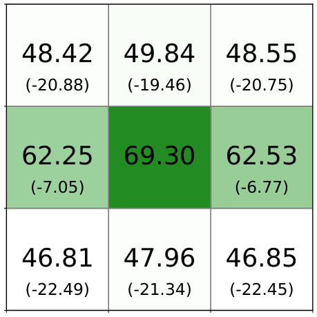
Experiment For each image, we have $9$ anchors (Fig. 1(b)) and the originally $K=36$ zoomed versions per anchor as defined in Section 3. Yet, after reducing to the minimum set (Section B.4), $K$ averages at $25$ , over all datasets, and $10\leq K\leq 31$ . Here, we count the probability that the $K$ zoomed versions per anchor lead to a correct prediction. In other words, we compute the upper-bound accuracy as in Section 4.1 but for each anchor separately.

Results First, as expected, the upper-bound accuracy for each anchor (Fig. 3) is consistently lower than when all $9$ anchors are allowed (Table 1c). Second, across all $6$ datasets, the center anchor consistently achieves the highest upper-bound accuracy versus the other $8$ locations (Fig. 3 and Section B.2), indicating a center bias in all datasets. However, we find this bias is small in IN, IN-R, and IN-S but large in IN-A and ON (i.e. the largest difference between center accuracy and the lowest off-center accuracy is around -25 and -23 points, respectively; whereas for other datasets, it is around (-1) to (-5) points, as shown in Fig. 3).

The center bias in ObjectNet can be explained by the fact that the images were captured using smartphones with aspect ratios of 2:3 or 9:16 (Section D.3.3). Overall, such strong center bias in IN-A and ON may not be desirable since improvements on these two benchmarks may be attributed to learning to zoom to the center as opposed to the intended quest of recognizing objects in unusual forms (IN-A) or poses (ON). By merely upscaling the image and center cropping, we can achieve higher accuracy using nearly all the same models on these two datasets (Figs. A14 and A17).

We also find that, during test time, center-zooming (Section B.5) increases the top-1 accuracy of all IN-trained models but not CLIP, even on IN-A and ON images. This observation is intriguing considering these OOD datasets contain more distracting objects than ImageNet images (Section C.2) and therefore, center-zooming should de-clutter the scene for more accurate classification. However, CLIP prefers a specific zoom scale that provides sufficient background for object recognition—it struggles to identify a single object in a tightly-cropped image [85]. Future research should examine whether this “zoom bias” of CLIP is due to its image- or text-encoder, or both.

4.3 Test-time augmentation of MEMO with only zoom-in transforms improves accuracy

Aggregating model predictions over zoom-in versions of the input image during test time leads to higher top-1 accuracy on IN, IN-ReaL, IN-A and ON, but lower accuracy on IN-R and IN-S (Section B.7). However, interestingly, always zooming out on IN-R and IN-S abstract images also hurts accuracy, suggesting that an adaptive zooming strategy might be a better approach.

Here, we test building such an adaptive test-time zooming strategy by modifying MEMO [83], a SOTA test-time augmentation method that finetunes a pre-trained classifier at test time to achieve a more accurate prediction. Specifically, MEMO finds a network that produces a low-entropy predicted label over a set of $K=16$ augmented versions of the test image $I$ and then runs this finetuned model on $I$ again to produce the final prediction. It does this by applying different augmentations to the test point $I$ to get augmented points $I_{1},\ldots,I_{K}$ , passing these through the model to obtain predictive distributions, and updating the model parameters by minimizing the entropy of the averaged marginal distribution over predictions. While improving accuracy, MEMO requires a pre-defined set of diverse augmentation transforms (e.g. sheer, rotate, and solarize in AugMix [26]). Yet, the hyperparameters for each type of transform are hard-coded, and the contribution of each transform to improved classification accuracy is unknown.

We improve MEMO’s accuracy and interpretability by replacing AugMix transforms with only zoom-in functions. Intuitively, a model first looks at all zoomed-in frames of the input image (at different zoom scales and locations) and then decides to achieve the most confident prediction.

Experiment MEMO relies on AugMix [25], which applies a set of 13 image transforms, such as translation, rotation, and color distortion, to an original image at varying intensities, and then chains them together to create $K=16$ new augmented images (examples in Section D.5).

We replace AugMix with RandomResizedCrop [4] (RRC), which takes a random crop of the input image (i.e. at a random location, random rectangular area, and a random aspect ratio) and then resizes it to the fixed 224 $\times$ 224 (i.e. the network input size). RRC basically implements a random zoom-in function (examples in Section D.5).

We compare the original MEMO [83] (which uses AugMix) and our version that uses RRC on five benchmarks (IN, IN-A, IN-R, IN-S, and ON). We follow the same experimental setup as in [83] (e.g. $K=16$ ). Specifically, we test three ResNet-50 variants that were pre-trained using distinct augmentation techniques.²² 2 The ResNet-50 model used as a baseline in this Section 4.3 is different from that in our other (non-MEMO) sections of the paper.

We utilize Grad-Cam [58] to understand the impact of MIMO on the network’s attentions within the final layer, both before and after modification. Specifically, our investigation seeks test our hypothesis concerning the model’s focus on the regions of interest within an image.

Results Both our MEMO + RRC and the original MEMO + AugMix [83] consistently outperform the baseline models, which do not use MEMO, on all five datasets (Table 2). That is, when combined with MEMO, zoom-in transforms implemented via RRC are also helpful in classifying IN-S and IN-R images—where we previously find zoom-in to not help in $\mathsf{mean}$ / $\mathsf{max}$ aggregation (Section B.7).

On average, over all three models and five datasets, our RRC outperforms AugMix by + $0.28$ points, with a larger impact on IN-A, where it achieves a mean improvement of + $1.10$ points (Table 2). Our results show that zoom-in alone can be a useful inductive bias, helping improve downstream image classification. In contrast, some of the transformations among the 13 transform functions in AugMix may not be essential to the results of Zhang et al. [83] (no ablation studies of transformations were provided in [83]) and are less effective than our zoom-in.

Table 2: MEMO + RRC (i.e. random zoom-in transforms) outperforms baselines and MEMO [83].

	Baseline (1-crop)					MEMO + AugMix [83]					MEMO + RRC (Ours)
	IN	IN-A	IN-R	IN-S	ON	IN	IN-A	IN-R	IN-S	ON	IN	IN-A	IN-R	IN-S	ON
ResNet-50 [23]	76.13	0.00	36.17	24.09	35.92	77.27	0.83	41.28	27.63	38.38	77.50	1.31	40.81	27.53	38.85
DeepAug+AugMix [26]	75.82	3.87	46.77	32.62	34.81	76.27	5.35	50.79	35.70	36.42	76.38	5.76	50.88	35.65	36.64
MoEx+CutMix [40]	79.04	7.97	35.52	23.96	38.59	79.38	11.21	40.65	27.07	40.62	79.49	13.61	40.41	26.80	41.43
mean $\pm$ std	36.75 $\pm$ 24.75					39.26 (+2.51) $\pm$ 24.32					39.54 (+2.79) $\pm$ 24.10

Figure 4 shows Grad-CAM visualizations for three samples, providing evidence of how the network’s behavior changes before and after the MEMO update. For an image of a pug, the network initially focused on a kitchen appliance, failing to detect the object correctly. After applying the MEMO modification, it refocused on the dog, classifying it accurately. Similarly, in an image of a fox squirrel, the network initially had a diffuse focus but refocused on the fox squirrel after the update. These results demonstrate the effectiveness of the MEMO modification in guiding the network’s attention or encouraging the model to perform an implicit zoom on the regions of interest, thereby improving its classification performance.

4.4 ImageNet-Hard: A benchmark with images that remain unclassifiable, even after 324 zoom attempts

Existing ImageNet-scale benchmarks followed one of the following three construction methods: (1) perturbing real images with the aim of making them harder for models to classify (e.g., ImageNet-C [24] and DAmageNet [13]); (2) collecting the real images that models misclassify (e.g., IN-A, ImageNet-O [27]); or (3) setting up a highly-controlled data collection process (e.g., IN-S and ON). Yet, none of such benchmarks explicitly challenge models on the ability to recognize a well-framed object in an image (i.e., no zooming required). For example, ON is supposed to test the recognition of objects in unusual poses but the cluttered background in ON images is actually a major reason for misclassification (Section 4.2). Furthermore, the results in Table 1 suggest that given optimal zooming, these existing benchmarks only challenge IN-trained models but not the Internet-scale vision-language models (e.g. CLIP) anymore. We propose ImageNet-Hard, a novel ImageNet-scale benchmark that challenges existing and future SOTA models. ImageNet-Hard is a collection of images that the SOTA CLIP-ViT-L/14 fails to correctly classify even when 324 zooming attempts are provided.

4.4.1 ImageNet-Hard construction

Initial data collection We take CLIP-ViT-L/14 (the highest-performing model in Table 1) and run the zooming procedure to find “Unclassifiable images” (defined in Section 4.1) from the following six datasets: IN-V2 [56], IN-ReaL, IN-A, IN-R, IN-S, and ON. That is, for each image $x$ , we generate 324 zoomed versions of $x$ and feed them into CLIP-ViT-L/14. We add $x$ to ImageNet-Hard only if none of the 324 versions are correctly classified.

Adding ImageNet-C The original IN-C [24] are the original IN images but center-cropped to 224 $\times$ 224 px, which significantly makes the classification task unnecessarily more ill-posed (e.g., by adding Gaussian noise to a crop where the main object is already removed).

To find a subset of IN-C images for adding into ImageNet-Hard, we first re-generate ImageNet-C by adding the 19 types of corruption noise to IN without resizing the original IN images. Second, we run CLIP-ViT-L/14 on all 19 corruption types and manually select a subset of six diverse and lowest-accuracy corruption groups: Impulse Noise, Frost, Fog, Snow, Brightness, and Zoom Blur. We repeat the initial data collection process for these 6 image sets of IN-C.

Groundtruth labels After the above procedure, our dataset contains 13,925 images collected from IN+ReaL, IN-V2, IN-A, IN-C, IN-R, IN-S, and ON (see the distribution in Section E.1). ImageNet-Hard presents a 1000-way classification task where the 1000 classes are from ImageNet. We manually inspect all images and remove 295 samples that are obviously ill-posed (e.g. an entirely black image but labeled great white shark in IN-S Fig. A60), arriving at a total of 13,630 ImageNet-Hard images. A sample contains only one groundtruth label from its original datasets except for IN and IN-C images, which have a set of IN+ReaL labels. Each IN or IN-C image is considered correctly labeled by a model if its top-1 predicted label is among the groundtruth labels.

Refining groundtruth labels via human feedback Label noise is still present in IN and OOD benchmarks despite cleaning efforts [10, 56, 81]. Since ImageNet-Hard contains images misclassified by CLIP-ViT-L/14, our manual inspection confirms many misclassified images have debatable labels.

To ameliorate the issue, we orchestrate a human feedback study for eliminating images with inaccurate labels. First, the first author examine every image and flag 3,133 images as ambiguous and needs verification. Then, we have two groups of annotators to help verify the labels (by choosing Accept, Reject, or Not Sure). Group A is composed of three students, each examine all 3,133 images where Group B is composed of 38 students, each examine 50 randomly-selected images. Our inter-annotator aggregation procedure merges labels from both groups and results in 2,280 images removed (out of 3,133 originally flagged), leaving ImageNet-Hard at a total of 11,350 images.

That is, we accept an image $x$ if one of the two conditions is satisfied: (1) when all 3/3 group-A annotators accept $x$ ; or (2) when 2/3 group-A annotators accept $x$ and all group-B reviewers of $x$ accept $x$ (assuming at least 1 group-B annotator reviews $x$ ; otherwise $x$ will be rejected).

Inspired by IN-ReaL [10], we further clean up the labels by eliminating 370 images associated with the labels sunglass, sunglasses, tub, bathtub, cradle, bassinet, projectile, and missile, i.e., the classes that often contain similar images that belong to more than one class. After this refinement, the final ImageNet-Hard dataset contains a total of 10,980 images.

4K version We utilize GigaGAN [33] to upscale every image in our final dataset and construct ImageNet-Hard-4K, which is aimed to facilitate future research into how a super-resolution step may improve image classification results (e.g., to classify an object when the image is blurry).

Release ImageNet-Hard and ImageNet-Hard-4K are released on HuggingFace (see samples in Fig. A49) under MIT License. Code for evaluating models on ImageNet-Hard is on GitHub.

4.4.2 ImageNet-Hard challenges SOTA classifiers, especially those operating at 224 $\times$ 224

Here, we evaluate the standard 1-crop, top-1 accuracy of SOTA classifiers on ImageNet-Hard. We use the image pre-processing function defined by each classifier. In addition to the 6 models in Section 4.1, we also test CLIP-ViT-L/14@336px [53], EfficientNet (B0@224px and B7@600px) [69], and EfficientNet-L2@800px [1]. CLIP-ViT-L/14@336px, EfficientNet-B7@600px, and EfficientNet-L2@800px are state-of-the-art models that operate at high resolutions of 336 $\times$ 336, 600 $\times$ 600, and 800 $\times$ 800 respectively. In addition, our evaluation includes models from the OpenCLIP family [30].

Results Table 3 shows fairly low top-1 accuracy by various classifiers on ImageNet-Hard. First, all well-known IN-trained classifiers that operate at 224 $\times$ 224 perform poorly between 7.34% (AlexNet) and 18.52% accuracy (ViT-B/32).

Since ImageNet-Hard is based on a collection of images that OpenAI’s CLIP ViT-L/14@224px mislabels, this classifier’s accuracy on our dataset is only 1.86%. Yet, interestingly, CLIP-ViT-L/14@336px also performs poorly at 2.02% (Table 3). Furthermore, all 68 tested OpenCLIP models perform poorly, with an accuracy below 16% (see details in Section E.6).

Separately, we observe a trend that models operating at a higher resolution tend to perform better on ImageNet-Hard with EfficientNet-L2@800px scoring highest at 39.00% (compared to 88.40% [79] on the original ImageNet). Overall, all models perform substantially worse on ImageNet-Hard (Table 3) than on other ImageNet-scale datasets (see Table A6; 1-crop). This result is expected because ImageNet-Hard is a set of hard cases collected from those OOD benchmarks.

ImageNet-Hard-4K We find that when upsampling images to 4K using GigaGAN [33] and downsampling them back to the resolution of each classifier does not help but even hurt the accuracy slightly (Table A13). Given that GigaGAN performs remarkably well, this result suggests ImageNet-Hard is different from typical fine-grained animal classification where improving the texture details increases classification accuracy [76]. The next section (Section 4.5) sheds light on model failures on ImageNet-Hard, revealing challenges posed to future SOTA models.

Table 3: Top-1 accuracy (%) on ImageNet-Hard of IN-trained models and those trained on larger, non-ImageNet datasets (black). All models operate at 224

\times

224 unless otherwise specify.

Classifier	Accuracy	Classifier	Accuracy	Classifier	Accuracy
AlexNet	7.34	ViT-B/32	18.52	CLIP-ViT-L/14@224px	1.86
VGG-16	12.00	EfficientNet-B0@224px	16.57	CLIP-ViT-L/14@336px	2.02
ResNet-18	10.86	EfficientNet-B7@600px	23.20	OpenCLIP-ViT-bigG-14	15.93
ResNet-50	14.74	EfficientNet-L2@800px	39.00	OpenCLIP-ViT-L-14	15.60

4.5 Analysis of Image Classification Errors

Motivated by the fact that EfficientNet-L2 is the best classifier on ImageNet-Hard, we qualitatively analyze its failure cases to characterize the challenge posed by our benchmark. Specifically, we provide gpt-3.5-turbo [51] with a pair of EfficientNet-L2’s top-1 (incorrect) label and the groundtruth label and ask it to categorize the error into “common” or “rare” based on the labels’ semantic similarity (see Section E.3 for full details). For instance, mislabeling bucket into barrel is common (as two objects are quite related) while mislabeling cloak into jigsaw puzzle is rare.

Results See Section E.4 for samples of wrong labels that EfficientNet-L2 most frequently misclassifies into. We find that 39.4% of EfficientNet-L2’s misclassifications on the ImageNet-Hard dataset are “common”, while 60.6% are “rare”.

A. Common group captures model confusion between two related classes (e.g. two fish species: clownfish and rock beauty; Fig. 5(a)). Yet, another source of problem for these “errors” is the debatable groundtruth labels, which may require domain-expert annotators to verify and rectify [45].

B. Rare group captures errors where the model confusion is between two semantically distant classes (e.g., llama $\to$ plectrum; Fig. 5(b)). This often happens with abstract images or objects in unusual poses [5] or forms [15]. Classifying this group of images is challenging and sometimes requires a strong understanding of context and reasoning capabilities.

5 Discussion and Conclusion

Limitations By manual inspection, we estimate 14.7% of labeling noise, which ImageNet-Hard inherits from the source datasets.

Our study rigorously analyzed the zooming effect on six known classifiers and image classification benchmarks. We first demonstrate that previous state-of-the-art classifiers, as old as AlexNet [38], could potentially achieve near $90\%$ accuracy with optimal zooming. This sparks the intriguing question of whether image classifiers’ evolution over the past ten years is about mastering where and at what scale to zoom (instead of enhancing feature extractors, a.k.a. representation learning [3]). Through another lens, we probe the evolution by analyzing the implicit zooming mechanisms that deep classifiers apply to input images. This perspective diverges from [54], which studied the progression of representation learning from CNNs to ViTs.

We are the first to document the spatial biases of existing benchmarks. Notably, IN-A and ON contain a large center bias and simply zooming to the center will de-clutter the scene and yield a high accuracy ( $24.69\%$ for ViT-B/32 on IN-A; Table A5), which is competitive with state-of-the-art trained models (e.g. $24.1\%$ of Robust ViT [11]) and much higher than state-of-the-art TTA techniques (e.g. $11.21\%$ of MEMO [83]; Table 2). Our simple, but strong zoom-in baselines on IN-A and ON motivate future research into better-controlled benchmarks that more explicitly test models on a set of pre-defined properties. Our proposed TTA method with zoom-in transforms (MEMO + RRC) is not only more accurate but also more interpretable and faster to run (Table A7) than the original MEMO.

Finally, we introduce ImageNet-Hard (Section 4.4), a new challenging dataset for SOTA IN-trained and vision-language classifiers.

Acknowledgement

GN is supported by Auburn University PGRF Fellowship. AN was supported by a NSF CAREER award No. 2145767, and donations from NaphCare Foundation, and Adobe Research. We greatly appreciate David Seunghyun Yoon’s help in generating the ImageNet-Hard-4K (Section 4.4.2) version using GigaGAN. We also thank those students at Auburn University and Alberta University who participated in our experiment for cleaning up the labels of ImageNet-Hard images.

References

[1] timm/tf_efficientnet_l2.ns_jft_in1k_475 · hugging face. https://huggingface.co/timm/tf_efficientnet_l2.ns_jft_in1k_475. (Accessed on 06/05/2023).
[2] Centercrop — torchvision main documentation. https://pytorch.org/vision/main/generated/torchvision.transforms.CenterCrop.html. (Accessed on 03/07/2023).
[3] Iclr 2023. https://iclr.cc/. (Accessed on 11/10/2022).
[4] Randomresizedcrop — torchvision main documentation. https://pytorch.org/vision/main/generated/torchvision.transforms.RandomResizedCrop.html. (Accessed on 03/08/2023).
Alcorn et al. [2019] Alcorn, M. A., Li, Q., Gong, Z., Wang, C., Mai, L., Ku, W.-S., and Nguyen, A. Strike (with) a pose: Neural networks are easily fooled by strange poses of familiar objects. In Proceedings of the IEEE/CVF conference on computer vision and pattern recognition, pp. 4845–4854, 2019.
Ayhan & Berens [2018] Ayhan, M. S. and Berens, P. Test-time data augmentation for estimation of heteroscedastic aleatoric uncertainty in deep neural networks. In Medical Imaging with Deep Learning, 2018.
Bahat & Shakhnarovich [2020] Bahat, Y. and Shakhnarovich, G. Classification confidence estimation with test-time data-augmentation. arXiv e-prints, pp. arXiv–2006, 2020.
Barbu et al. [2019] Barbu, A., Mayo, D., Alverio, J., Luo, W., Wang, C., Gutfreund, D., Tenenbaum, J., and Katz, B. Objectnet: A large-scale bias-controlled dataset for pushing the limits of object recognition models. Advances in neural information processing systems, 32, 2019.
Bau et al. [2017] Bau, D., Zhou, B., Khosla, A., Oliva, A., and Torralba, A. Network dissection: Quantifying interpretability of deep visual representations. In Proceedings of the IEEE conference on computer vision and pattern recognition, pp. 6541–6549, 2017.
Beyer et al. [2020] Beyer, L., Hénaff, O. J., Kolesnikov, A., Zhai, X., and Oord, A. v. d. Are we done with imagenet? arXiv preprint arXiv:2006.07159, 2020.
Chefer et al. [2022] Chefer, H., Schwartz, I., and Wolf, L. Optimizing relevance maps of vision transformers improves robustness. In Oh, A. H., Agarwal, A., Belgrave, D., and Cho, K. (eds.), Advances in Neural Information Processing Systems, 2022. URL https://openreview.net/forum?id=upuYKQiyxa_.
Chen et al. [2020] Chen, P., Agarwal, C., and Nguyen, A. The shape and simplicity biases of adversarially robust imagenet-trained cnns. arXiv preprint arXiv:2006.09373, 2020.
Chen et al. [2019] Chen, S., Huang, X., He, Z., and Sun, C. Damagenet: A universal adversarial dataset. arXiv preprint arXiv:1912.07160, 2019.
Chun et al. [2022] Chun, S., Lee, J. Y., and Kim, J. Cyclic test time augmentation with entropy weight method. In Uncertainty in Artificial Intelligence, pp. 433–442. PMLR, 2022.
De Vries et al. [2019] De Vries, T., Misra, I., Wang, C., and Van der Maaten, L. Does object recognition work for everyone? In Proceedings of the IEEE/CVF conference on computer vision and pattern recognition workshops, pp. 52–59, 2019.
Donnelly et al. [2022] Donnelly, J., Barnett, A. J., and Chen, C. Deformable protopnet: An interpretable image classifier using deformable prototypes. In Proceedings of the IEEE/CVF Conference on Computer Vision and Pattern Recognition, pp. 10265–10275, 2022.
Dosovitskiy et al. [2020] Dosovitskiy, A., Beyer, L., Kolesnikov, A., Weissenborn, D., Zhai, X., Unterthiner, T., Dehghani, M., Minderer, M., Heigold, G., Gelly, S., et al. An image is worth 16x16 words: Transformers for image recognition at scale. In International Conference on Learning Representations, 2020.
Fu et al. [2017] Fu, J., Zheng, H., and Mei, T. Look closer to see better: Recurrent attention convolutional neural network for fine-grained image recognition. In Proceedings of the IEEE conference on computer vision and pattern recognition, pp. 4438–4446, 2017.
Geirhos et al. [2019] Geirhos, R., Rubisch, P., Michaelis, C., Bethge, M., Wichmann, F. A., and Brendel, W. Imagenet-trained CNNs are biased towards texture; increasing shape bias improves accuracy and robustness. In International Conference on Learning Representations, 2019. URL https://openreview.net/forum?id=Bygh9j09KX.
Geirhos et al. [2020] Geirhos, R., Jacobsen, J.-H., Michaelis, C., Zemel, R., Brendel, W., Bethge, M., and Wichmann, F. A. Shortcut learning in deep neural networks. Nature Machine Intelligence, 2(11):665–673, 2020.
Goh et al. [2021] Goh, G., Cammarata, N., Voss, C., Carter, S., Petrov, M., Schubert, L., Radford, A., and Olah, C. Multimodal neurons in artificial neural networks. Distill, 6(3):e30, 2021.
Gupta et al. [2019] Gupta, A., Dollar, P., and Girshick, R. Lvis: A dataset for large vocabulary instance segmentation. In Proceedings of the IEEE/CVF conference on computer vision and pattern recognition, pp. 5356–5364, 2019.
He et al. [2016] He, K., Zhang, X., Ren, S., and Sun, J. Deep residual learning for image recognition. In Proceedings of the IEEE conference on computer vision and pattern recognition, pp. 770–778, 2016.
Hendrycks & Dietterich [2019] Hendrycks, D. and Dietterich, T. Benchmarking neural network robustness to common corruptions and perturbations. arXiv preprint arXiv:1903.12261, 2019.
Hendrycks et al. [2019] Hendrycks, D., Mu, N., Cubuk, E. D., Zoph, B., Gilmer, J., and Lakshminarayanan, B. Augmix: A simple data processing method to improve robustness and uncertainty. arXiv preprint arXiv:1912.02781, 2019.
Hendrycks et al. [2021a] Hendrycks, D., Basart, S., Mu, N., Kadavath, S., Wang, F., Dorundo, E., Desai, R., Zhu, T., Parajuli, S., Guo, M., et al. The many faces of robustness: A critical analysis of out-of-distribution generalization. In Proceedings of the IEEE/CVF International Conference on Computer Vision, pp. 8340–8349, 2021a.
Hendrycks et al. [2021b] Hendrycks, D., Zhao, K., Basart, S., Steinhardt, J., and Song, D. Natural adversarial examples. In Proceedings of the IEEE/CVF Conference on Computer Vision and Pattern Recognition, pp. 15262–15271, 2021b.
Howard et al. [2019] Howard, A., Sandler, M., Chu, G., Chen, L.-C., Chen, B., Tan, M., Wang, W., Zhu, Y., Pang, R., Vasudevan, V., et al. Searching for mobilenetv3. In Proceedings of the IEEE/CVF international conference on computer vision, pp. 1314–1324, 2019.
Huang et al. [2017] Huang, G., Liu, Z., Van Der Maaten, L., and Weinberger, K. Q. Densely connected convolutional networks. In Proceedings of the IEEE conference on computer vision and pattern recognition, pp. 4700–4708, 2017.
Ilharco et al. [2021] Ilharco, G., Wortsman, M., Wightman, R., Gordon, C., Carlini, N., Taori, R., Dave, A., Shankar, V., Namkoong, H., Miller, J., Hajishirzi, H., Farhadi, A., and Schmidt, L. Openclip, July 2021. URL https://doi.org/10.5281/zenodo.5143773. If you use this software, please cite it as below.
Jaderberg et al. [2015] Jaderberg, M., Simonyan, K., Zisserman, A., et al. Spatial transformer networks. Advances in neural information processing systems, 28, 2015.
Jin et al. [2021] Jin, C., Tanno, R., Mertzanidou, T., Panagiotaki, E., and Alexander, D. C. Learning to downsample for segmentation of ultra-high resolution images. arXiv preprint arXiv:2109.11071, 2021.
Kang et al. [2023] Kang, M., Zhu, J.-Y., Zhang, R., Park, J., Shechtman, E., Paris, S., and Park, T. Scaling up gans for text-to-image synthesis. arXiv preprint arXiv:2303.05511, 2, 2023.
Kim et al. [2020] Kim, I., Kim, Y., and Kim, S. Learning loss for test-time augmentation. Advances in Neural Information Processing Systems, 33:4163–4174, 2020.
Kleinberg & Tardos [2005] Kleinberg, J. and Tardos, E. Algorithm Design. Addison-Wesley Longman Publishing Co., Inc., USA, 2005. ISBN 0321295358.
Kong & Henao [2022] Kong, F. and Henao, R. Efficient classification of very large images with tiny objects. In Proceedings of the IEEE/CVF Conference on Computer Vision and Pattern Recognition, pp. 2384–2394, 2022.
Krause et al. [2015] Krause, J., Jin, H., Yang, J., and Fei-Fei, L. Fine-grained recognition without part annotations. In Proceedings of the IEEE conference on computer vision and pattern recognition, pp. 5546–5555, 2015.
Krizhevsky et al. [2012] Krizhevsky, A., Sutskever, I., and Hinton, G. E. Imagenet classification with deep convolutional neural networks. Advances in neural information processing systems, 25, 2012.
Leung et al. [2021] Leung, B., Ho, C.-H., Persekian, A., Orozco, D., Chang, Y., Sandstrom, E., Liu, B., and Vasconcelos, N. Oowl500: Overcoming dataset collection bias in the wild. arXiv preprint arXiv:2108.10992, 2021.
Li et al. [2021a] Li, B., Wu, F., Lim, S.-N., Belongie, S., and Weinberger, K. Q. On feature normalization and data augmentation. In Proceedings of the IEEE/CVF Conference on Computer Vision and Pattern Recognition, pp. 12383–12392, 2021a.
Li et al. [2021b] Li, J., Xiong, C., and Hoi, S. C. Learning from noisy data with robust representation learning. In Proceedings of the IEEE/CVF International Conference on Computer Vision, pp. 9485–9494, 2021b.
Li et al. [2021c] Li, X., Li, J., Dai, T., Shi, J., Zhu, J., and Hu, X. Rethinking natural adversarial examples for classification models. arXiv preprint arXiv:2102.11731, 2021c.
Liu et al. [2021] Liu, Z., Lin, Y., Cao, Y., Hu, H., Wei, Y., Zhang, Z., Lin, S., and Guo, B. Swin transformer: Hierarchical vision transformer using shifted windows. In Proceedings of the IEEE/CVF international conference on computer vision, pp. 10012–10022, 2021.
Liu et al. [2022] Liu, Z., Mao, H., Wu, C.-Y., Feichtenhofer, C., Darrell, T., and Xie, S. A convnet for the 2020s. In Proceedings of the IEEE/CVF Conference on Computer Vision and Pattern Recognition, pp. 11976–11986, 2022.
Luccioni & Rolnick [2022] Luccioni, A. S. and Rolnick, D. Bugs in the data: How imagenet misrepresents biodiversity. arXiv preprint arXiv:2208.11695, 2022.
Lyzhov et al. [2020] Lyzhov, A., Molchanova, Y., Ashukha, A., Molchanov, D., and Vetrov, D. Greedy policy search: A simple baseline for learnable test-time augmentation. In Conference on Uncertainty in Artificial Intelligence, pp. 1308–1317. PMLR, 2020.
Ma et al. [2018] Ma, N., Zhang, X., Zheng, H.-T., and Sun, J. Shufflenet v2: Practical guidelines for efficient cnn architecture design. In Proceedings of the European conference on computer vision (ECCV), pp. 116–131, 2018.
Marcel & Rodriguez [2010] Marcel, S. and Rodriguez, Y. Torchvision the machine-vision package of torch. In Proceedings of the 18th ACM international conference on Multimedia, pp. 1485–1488, 2010.
Minderer et al. [2022] Minderer, M., Gritsenko, A., Stone, A., Neumann, M., Weissenborn, D., Dosovitskiy, A., Mahendran, A., Arnab, A., Dehghani, M., Shen, Z., et al. Simple open-vocabulary object detection with vision transformers. arXiv preprint arXiv:2205.06230, 2022.
Nguyen et al. [2016] Nguyen, A., Yosinski, J., and Clune, J. Multifaceted feature visualization: Uncovering the different types of features learned by each neuron in deep neural networks. arXiv preprint arXiv:1602.03616, 2016.
OpenAI [2023] OpenAI. Chatgpt api. https://openai.com/blog/chatgpt, 2023.
Pang et al. [2019] Pang, T., Xu, K., and Zhu, J. Mixup inference: Better exploiting mixup to defend adversarial attacks. arXiv preprint arXiv:1909.11515, 2019.
Radford et al. [2021] Radford, A., Kim, J. W., Hallacy, C., Ramesh, A., Goh, G., Agarwal, S., Sastry, G., Askell, A., Mishkin, P., Clark, J., et al. Learning transferable visual models from natural language supervision. In International conference on machine learning, pp. 8748–8763. PMLR, 2021.
Raghu et al. [2021] Raghu, M., Unterthiner, T., Kornblith, S., Zhang, C., and Dosovitskiy, A. Do vision transformers see like convolutional neural networks? Advances in Neural Information Processing Systems, 34:12116–12128, 2021.
Recasens et al. [2018] Recasens, A., Kellnhofer, P., Stent, S., Matusik, W., and Torralba, A. Learning to zoom: a saliency-based sampling layer for neural networks. In Proceedings of the European Conference on Computer Vision (ECCV), pp. 51–66, 2018.
Recht et al. [2019] Recht, B., Roelofs, R., Schmidt, L., and Shankar, V. Do imagenet classifiers generalize to imagenet? In International conference on machine learning, pp. 5389–5400. PMLR, 2019.
Robinson et al. [2021] Robinson, J., Sun, L., Yu, K., Batmanghelich, K., Jegelka, S., and Sra, S. Can contrastive learning avoid shortcut solutions? Advances in neural information processing systems, 34:4974–4986, 2021.
Rs et al. [2020] Rs, R., Cogswell, M., Das, A., Vedantam, R., Parikh, D., and Batra, D. Grad-cam: Visual explanations from deep networks via gradient-based localization. International Journal of Computer Vision, 128, 02 2020. doi: 10.1007/s11263-019-01228-7.
Russakovsky et al. [2015] Russakovsky, O., Deng, J., Su, H., Krause, J., Satheesh, S., Ma, S., Huang, Z., Karpathy, A., Khosla, A., Bernstein, M., et al. Imagenet large scale visual recognition challenge. International Journal of Computer Vision, 115(3):211–252, 2015.
Sandler et al. [2018] Sandler, M., Howard, A., Zhu, M., Zhmoginov, A., and Chen, L.-C. Mobilenetv2: Inverted residuals and linear bottlenecks. In Proceedings of the IEEE conference on computer vision and pattern recognition, pp. 4510–4520, 2018.
Sato et al. [2015] Sato, I., Nishimura, H., and Yokoi, K. Apac: Augmented pattern classification with neural networks. arXiv preprint arXiv:1505.03229, 2015.
Shanmugam et al. [2021] Shanmugam, D., Blalock, D., Balakrishnan, G., and Guttag, J. Better aggregation in test-time augmentation. In Proceedings of the IEEE/CVF International Conference on Computer Vision, pp. 1214–1223, 2021.
Simonyan & Zisserman [2014] Simonyan, K. and Zisserman, A. Very deep convolutional networks for large-scale image recognition. arXiv preprint arXiv:1409.1556, 2014.
Slavík [1996] Slavík, P. A tight analysis of the greedy algorithm for set cover. In Proceedings of the Twenty-Eighth Annual ACM Symposium on Theory of Computing, STOC ’96, pp. 435–441, New York, NY, USA, 1996. Association for Computing Machinery. ISBN 0897917855. doi: 10.1145/237814.237991. URL https://doi.org/10.1145/237814.237991.
Smith & Gal [2018] Smith, L. and Gal, Y. Understanding measures of uncertainty for adversarial example detection. arXiv preprint arXiv:1803.08533, 2018.
Steiner et al. [2021] Steiner, A., Kolesnikov, A., Zhai, X., Wightman, R., Uszkoreit, J., and Beyer, L. How to train your vit? data, augmentation, and regularization in vision transformers. arXiv preprint arXiv:2106.10270, 2021.
Szegedy et al. [2015] Szegedy, C., Liu, W., Jia, Y., Sermanet, P., Reed, S., Anguelov, D., Erhan, D., Vanhoucke, V., and Rabinovich, A. Going deeper with convolutions. In Proceedings of the IEEE conference on computer vision and pattern recognition, pp. 1–9, 2015.
Taesiri et al. [2022] Taesiri, M. R., Nguyen, G., and Nguyen, A. Visual correspondence-based explanations improve ai robustness and human-ai team accuracy. Advances in Neural Information Processing Systems, 35:34287–34301, 2022.
Tan & Le [2019] Tan, M. and Le, Q. Efficientnet: Rethinking model scaling for convolutional neural networks. In International conference on machine learning, pp. 6105–6114. PMLR, 2019.
Thavamani et al. [2023] Thavamani, C., Li, M., Ferroni, F., and Ramanan, D. Learning to zoom and unzoom. In Proceedings of the IEEE/CVF Conference on Computer Vision and Pattern Recognition, pp. 5086–5095, 2023.
Tsipras et al. [2020] Tsipras, D., Santurkar, S., Engstrom, L., Ilyas, A., and Madry, A. From imagenet to image classification: Contextualizing progress on benchmarks. In International Conference on Machine Learning, pp. 9625–9635. PMLR, 2020.
Tu et al. [2022] Tu, Z., Talebi, H., Zhang, H., Yang, F., Milanfar, P., Bovik, A., and Li, Y. Maxvit: Multi-axis vision transformer. In European conference on computer vision, pp. 459–479. Springer, 2022.
Uzkent & Ermon [2020] Uzkent, B. and Ermon, S. Learning when and where to zoom with deep reinforcement learning. In Proceedings of the IEEE/CVF conference on computer vision and pattern recognition, pp. 12345–12354, 2020.
Wang et al. [2020] Wang, D., Shelhamer, E., Liu, S., Olshausen, B., and Darrell, T. Tent: Fully test-time adaptation by entropy minimization. In International Conference on Learning Representations, 2020.
Wang et al. [2019] Wang, H., Ge, S., Lipton, Z., and Xing, E. P. Learning robust global representations by penalizing local predictive power. Advances in Neural Information Processing Systems, 32, 2019.
Wei et al. [2021] Wei, X.-S., Song, Y.-Z., Mac Aodha, O., Wu, J., Peng, Y., Tang, J., Yang, J., and Belongie, S. Fine-grained image analysis with deep learning: A survey. IEEE transactions on pattern analysis and machine intelligence, 44(12):8927–8948, 2021.
Wightman et al. [2021] Wightman, R., Touvron, H., and Jégou, H. Resnet strikes back: An improved training procedure in timm. arXiv preprint arXiv:2110.00476, 2021.
Xiao et al. [2020] Xiao, K. Y., Engstrom, L., Ilyas, A., and Madry, A. Noise or signal: The role of image backgrounds in object recognition. In International Conference on Learning Representations, 2020.
Xie et al. [2020] Xie, Q., Luong, M.-T., Hovy, E., and Le, Q. V. Self-training with noisy student improves imagenet classification. In Proceedings of the IEEE/CVF conference on computer vision and pattern recognition, pp. 10687–10698, 2020.
Xie et al. [2017] Xie, S., Girshick, R., Dollár, P., Tu, Z., and He, K. Aggregated residual transformations for deep neural networks. In Proceedings of the IEEE conference on computer vision and pattern recognition, pp. 1492–1500, 2017.
Yun et al. [2021] Yun, S., Oh, S. J., Heo, B., Han, D., Choe, J., and Chun, S. Re-labeling imagenet: from single to multi-labels, from global to localized labels. In Proceedings of the IEEE/CVF Conference on Computer Vision and Pattern Recognition, pp. 2340–2350, 2021.
Zagoruyko & Komodakis [2016] Zagoruyko, S. and Komodakis, N. Wide residual networks. arXiv preprint arXiv:1605.07146, 2016.
Zhang et al. [2021] Zhang, M., Levine, S., and Finn, C. Memo: Test time robustness via adaptation and augmentation. arXiv preprint arXiv:2110.09506, 2021.
Zheng et al. [2019] Zheng, H., Fu, J., Zha, Z.-J., and Luo, J. Looking for the devil in the details: Learning trilinear attention sampling network for fine-grained image recognition. In Proceedings of the IEEE/CVF Conference on Computer Vision and Pattern Recognition, pp. 5012–5021, 2019.
Zhong et al. [2022] Zhong, Y., Yang, J., Zhang, P., Li, C., Codella, N., Li, L. H., Zhou, L., Dai, X., Yuan, L., Li, Y., et al. Regionclip: Region-based language-image pretraining. In Proceedings of the IEEE/CVF Conference on Computer Vision and Pattern Recognition, pp. 16793–16803, 2022.
Zhu et al. [2016] Zhu, Z., Xie, L., and Yuille, A. L. Object recognition with and without objects. arXiv preprint arXiv:1611.06596, 2016.

Appendix for:
ImageNet-Hard: The Hardest Images Remaining from a Study of the Power of Zoom and Spatial Biases in Image Classification

Appendix A Implementation details

In this section, we provide a detailed description of our experimental setup, including the Python code for our zoom transform, the classifiers we employed, and the setup we used for zero-shot classification.

A.1 Sample Python code for zoom-based transform

⬇ from PIL import Image import torchvision.transforms.functional as fv import torchvision.transforms as transforms from functools import partial def crop_at(size, slice_x, slice_y): def slice_crop(image, size, slice_x, slice_y): width, height = image.size tile_size_x = width // 3 tile_size_y = height // 3 anchor_x = (slice_y * tile_size_x) + (tile_size_x // 2) anchor_y = (slice_x * tile_size_y) + (tile_size_y // 2) return fv.crop( image, anchor_y - (size // 2), anchor_x - (size // 2), size, size, ) return partial(slice_crop, size=size, slice_x=slice_x, slice_y=slice_y) zoom_scale = 255 zoom_transform = transforms.Compose( [ transforms.Resize( zoom_scale, interpolation=transforms.InterpolationMode.BICUBIC, max_size=None, antialias=None, ), crop_at(224, i, j), ] )

Figure A1: Sample python code.

A.2 Datasets’ licenses

Dataset Name	License
ImageNet	Custom license, non-commercial
ImageNet-A	License
ImageNet-R	MIT License
ImageNet-Sketch	MIT License
ImageNet-C	MIT License
ObjectNet	Custom license derived from Creative Commons Attribution 4.0
ImageNet-V2	MIT License

Table A1: Dataset Licenses

A.3 Zoom Scales used

In our experiments, we tried the following zoom scales:

		$\displaystyle 10,16,32,48,64,96,122,128,192,224,235,240,256,288,320,348,384,448,460,512,$
		$\displaystyle 573,576,640,664,672,680,686,690,700,720,768,798,832,896,911,1024.$

A.4 Model selection

We use the official OpenAI’s official CLIP for all CLIP-related experiments. All IN-trained models are retrieved from the torchvision [48] library. For models from the OpenCLIP family, we utilize the OpenCLIP library version 2.20.0. In the case of the EfficientNet-B family, we use the Hugging Face Transformers library. Lastly, for EfficientNet-L2, we use the implementation from the timm library.

A.5 Zero-shot classification using CLIP

For CLIP, we follow the standard zero-shot classification. This involves creating a text template for each class in the dataset, which contains a generic description of an image featuring an object from that class. Then, we use CLIP’s text encoder to obtain embeddings for these templates and then average them to obtain a final vector that represents the class. To classify an image, we calculate the cosine similarity between its embedding and the text vectors for each class and then select the class with the highest value.

A.6 Zoom-based transform

Appendix B Additional Results

In this section, we provide additional results for our experiments.

B.1 Zooming out is needed for a small portion of the datasets

In our approach, we leverage the power of both zoom-in and zoom-out transforms, and Table 1 results indicate that this combined zooming approach can be effective in classifying images from diverse datasets. Zooming in enhances texture patterns while zooming out provides a better perspective of the object’s shape. The question we aim to answer is which dataset and model pairs require which type of zoom, and whether zooming is always necessary. Additionally, we investigate which types of networks are less reliant on explicit zooming, as they implicitly focus on the main object in the image.

Experiment

We separate zoom transforms into three groups and report the maximum possible accuracy as defined in Section 3. We use transforms in the minimum set covers (as shown in Fig. A10) for each dataset and classifier pair. We then report the number of images that can only be classified using transforms in each group separately.

Results

In general, we find that zooming in is more effective than zooming out. Zooming in provides two benefits: (1) it helps the model to focus on the key region where the target object is located, and (2) the model can extract features from the target object at a higher resolution. Across all methods and datasets, we can see a certain percentage of images are only classifiable using transforms of the zoom-out group. In particular, for ImageNet-R and ImageNet-Sketch, between $1.2\%-3$ % (Table A2) of the entire dataset can only be solved using a transform in the zoom-out group. This is especially true for drawings, where the texture may lack distinguishable features, and zooming out allows us to better perceive the shape.

Table A2: Breakdown of maximum possible accuracy by different zoom groups. In each dataset, certain images necessitate a specific zoom group for correct classification regardless of the model being used. However, CLIP performs well overall without depending heavily on a particular zoom level. On average, the percentage of datasets that can only be solved with a specific zoom group is very small for this model.

Dataset

Model

zoom-in

Solve

zoom-out

Solves

zoom-224

Solves

Only zoom-in

Solves

Only zoom-out

Solves

Only zoom-224

Solves

ImageNet

ResNet-18

94.57

79.49

81.16

10.59

0.43

0.08

ResNet-50

96.30

85.84

86.39

7.59

0.40

0.04

ViT-B/32

96.83

86.18

85.12

7.59

0.30

0.02

VGG-16

94.60

82.11

83.08

8.92

0.58

0.07

AlexNet

89.17

62.92

67.98

18.01

0.65

0.18

CLIP-ViT-L/14

95.82

90.80

87.04

4.81

0.83

0.05

ImageNet ReaL

ResNet-18

97.37

86.10

87.62

7.38

0.27

0.07

ResNet-50

98.22

91.07

91.87

4.65

0.25

0.04

ViT-B/32

98.50

90.79

88.06

4.92

0.18

0.03

VGG-16

97.38

88.43

89.40

6.02

0.38

0.07

AlexNet

93.15

69.58

74.85

15.47

0.45

0.19

CLIP-ViT-L/14

98.05

94.44

91.69

3.20

0.55

0.04

ImageNet+ReaL

ResNet-18

97.16

85.51

86.77

7.72

0.28

0.05

ResNet-50

98.25

91.10

91.77

4.60

0.24

0.03

ViT-B/32

98.70

91.00

90.95

4.92

0.14

0.02

VGG-16

97.12

87.88

89.09

6.25

0.42

0.06

AlexNet

92.79

68.65

73.93

16.25

0.47

0.16

CLIP-ViT-L/14

98.24

95.09

92.41

2.75

0.47

0.04

ImageNet-A

ResNet-18

63.66

47.95

45.37

13.97

2.75

0.21

ResNet-50

65.28

52.36

48.59

12.05

3.13

0.22

ViT-B/32

73.07

56.34

54.84

14.20

2.04

0.27

VGG-16

56.67

44.95

39.35

11.80

3.85

0.24

AlexNet

52.69

32.86

31.95

17.15

2.34

0.30

CLIP-ViT-L/14

98.35

96.71

93.57

1.70

0.69

0.04

ImageNet-R

ResNet-18

57.07

12.19

10.07

40.67

0.92

0.19

ResNet-50

64.52

12.95

10.36

48.72

1.00

0.23

ViT-B/32

76.71

18.57

21.92

51.75

0.85

0.15

VGG-16

56.59

13.15

13.27

38.24

0.93

0.29

AlexNet

39.91

10.39

9.11

26.27

1.08

0.36

CLIP-ViT-L/14

97.99

81.32

77.03

12.01

0.44

0.05

ImageNet-Sketch

ResNet-18

41.14

27.06

27.41

11.83

1.77

0.36

ResNet-50

44.72

32.80

31.45

10.99

2.23

0.24

ViT-B/32

53.45

37.43

37.38

13.11

1.83

0.36

VGG-16

36.20

27.20

24.59

9.47

2.97

0.28

AlexNet

27.71

13.84

15.11

11.26

1.22

0.33

CLIP-ViT-L/14

86.20

80.67

73.94

6.64

2.38

0.12

ObjectNet

ResNet-18

68.98

38.52

37.23

25.76

1.93

0.25

ResNet-50

74.16

51.56

47.79

19.68

2.16

0.30

ViT-B/32

77.66

44.49

42.65

27.43

1.34

0.20

VGG-16

69.19

41.72

39.49

23.34

2.27

0.31

AlexNet

56.76

23.45

22.59

28.85

2.27

0.33

CLIP-ViT-L/14

91.28

82.22

77.60

8.37

1.38

0.15

Average

ResNet-18

74.28

53.83

53.66

16.85

1.19

0.17

ResNet-50

77.35

59.67

58.32

15.47

1.34

0.16

ViT-B/32

82.13

60.69

60.13

17.70

0.95

0.15

VGG-16

72.54

55.06

54.04

14.86

1.63

0.19

AlexNet

64.60

40.24

42.22

19.04

1.21

0.26

CLIP-ViT-L/14

95.13

88.75

84.75

5.64

0.95

0.07

B.2 Anchor-based analysis of Center bias in ImageNet and OOD datasets

B.3 Distribution of the minimum set cover per classifier and dataset

In this section, we provide details on the distribution of minimum set cover size.

Table A3: Distribution of the minimum set cover per classifier and dataset. (ZI: zoom-in, ZO: zoom-out, ZL: zoom-224)

	ReaL				IN-A				IN-R				IN-Sketch				ON
	ZI	ZO	ZL	Total	ZI	ZO	ZL	Total	ZI	ZO	ZL	Total	ZI	ZO	ZL	Total	ZI	ZO	ZL	Total
ResNet-18	160	33	8	201	174	31	6	211	204	65	9	278	209	51	9	269	191	54	9	254
ResNet-50	136	33	9	178	165	42	7	214	200	62	9	271	216	56	9	281	187	63	9	259
ViT-B/32	134	30	4	168	167	19	7	193	196	52	9	257	218	46	9	273	206	58	9	273
VGG-16	158	34	9	201	181	33	8	222	214	66	9	289	210	54	9	273	198	52	9	259
AlexNet	191	40	8	239	170	33	9	212	212	51	9	272	217	49	9	275	201	58	9	268
CLIP-ViT-L/14	141	48	8	197	75	14	4	93	76	33	5	114	142	61	9	212	205	66	9	280

B.4 Only $70\%$ of all transforms are needed to reach maximum possible accuracy

In Section 4.1, we first pre-define all $324$ zoom transforms and then compute the maximum possible accuracy to ensure the predicted labels were the results of models looking at a controlled zoomed region (i.e. not because a model was given $324$ arbitrary trials per image). Here, we aim to compute the minimum number of zoom settings required for a model to reach the same upper-bound accuracy. Evaluating this minimum set may reveal spatial biases of a dataset (Section 4.2) as well as the implicit zoom operation that a state-of-the-art model (e.g. CLIP) may have learned.

Experiment Given a (dataset, classifier) pair, we constructed a bipartite graph $G=(N,E)$ , where $N=A\cup B$ , $A$ represents the set of transforms, and $B$ represents the set of images. The edges $E$ are defined as follows:

E=\{(n_{i},n_{j})\mid n_{i}\in A,n_{j}\in B,\text{ and transform }n_{i}\text{ leads to the correct classification of image }n_{j}\}

We aim to find a minimum set cover [64, 35] in this graph, synonymous with finding a minimum subset of transforms among the $324$ that lead to the correct prediction for all classifiable images in Section 4 (i.e. those that make up the accuracy scores in Table 1c), without unnecessary transforms.

The resulting subset of transforms from the process leads to the correct prediction for all classifiable images without sacrificing accuracy. During each iteration of the greedy minimum set cover algorithm, the transform that yields the highest number of correct classifications for the remaining images is selected. This process continues until all of the images have been “covered,” i.e. all images have connected to a transform with at least one edge. The result aligns with our initial goal to remove unnecessary zoom transforms while maintaining the maximum possible accuracy, as outlined in Section 4 (i.e., those that make up the accuracy scores in Table 1c). The outline of the algorithm can be seen in Algorithm 1.

Algorithm 1 Greedy Minimum Set Cover for Transforms

1: Initialization:

C=\emptyset

(Covered set of images),

T=\emptyset

(Selected transforms)

2: while

C\neq B

3: Find

n_{i}\in A\setminus T

that maximizes

|n_{j}\in B\setminus C\mid(n_{i},n_{j})\in E|

C=C\cup\{n_{j}\mid(n_{i},n_{j})\in E\}

T=T\cup\{n_{i}\}

6: end while

7: Result: The subset of transforms corresponding to

T

can classify images without sacrificing accuracy.

Figure A10: The minimum number of zoom transforms (out of 324) required to achieve the maximum possible accuracy scores reported in Table 1c.

	IN	ReaL	IN+ReaL	IN-A	IN-R	IN-S	ON	$\mu$
AlexNet	255	239	246	212	272	275	268	252
VGG-16	242	201	201	222	289	273	259	241
ResNet-18	250	201	208	211	278	269	254	239
ResNet-50	234	178	183	214	271	281	259	231
ViT-B/32	233	168	173	193	257	273	273	224
CLIP-ViT-L/14	251	197	186	93	114	280	212	190

Results Fig. A10 shows the minimum number of transforms per dataset required to reach the maximum possible accuracy. Although this number varies depending on the dataset and classifier, on average, the size of the minimum cover is $229$ , which is $\sim$ 70% of all $324$ pre-defined transforms.

We evaluate the maximum possible accuracy using the top 36 transforms, the same number as the number of zoom scales and report the results in Table 1b. This set of transforms is achieved by stopping the algorithm after 36 iterations, which provided us with 36 high-performing transforms. The maximum possible accuracy using only 36 crops is only slightly lower than that when using all $324$ crops but is substantially higher than the standard 1-crop, e.g. $85.19\%$ vs. $56.16\%$ for AlexNet on IN (Table 1b). Also, the upper-bound accuracy for 36 crops being much higher than the random baseline (i.e. $3.6\%$ for IN) confirms that the pre-defined zoom transforms are important to classification (not because models are given 36 random trials per image). The top-36 zoom transforms for ResNet-50 on ImageNet contain zooms at various locations in the image (see the visualizations in Section D.1).

Remarkably, CLIP requires 190 transforms on average, which is fewer than every other model (Fig. A10; $\mu$ column). This can be attributed to either the implicit zoom power of CLIP or the fact it has a stronger feature extractor.

B.5 Center-zooming increases the accuracy of all ImageNet-trained models but not CLIP

Previously, we have found that CLIP obtains the best accuracy on all six datasets (Table 1a) and also requires the smallest minimum set of zoom transforms to obtain the upper-bound accuracy (Section B.4). It is important to understand what classification strategy a CLIP classifier internally performs to classify better. Here, we test the hypothesis that the state-of-the-art CLIP is already performing an implicit zoom on images. If that is true, directly zooming to the center, exploiting the strong center bias of ImageNet-A and ObjectNet, will not improve CLIP accuracy.

Experiment We evaluate the accuracy of all models when center-zooming on IN-A and ON images at 11 different scales $S\in\{128,160,192,...,448\}$ (Fig. A11). That is, center-zooming at $S$ first resizes the input image so that the smaller dimension becomes $S$ and then takes a 224 $\times$ 224 center crop (zero-padding is applied when necessary).

Results In Fig. A11, we show the changes in the top-1 accuracy (1-crop) when varying the center-zoom scales away from the default ImageNet transform scale ( $S=256$ ) for both ImageNet-A and ObjectNet. While IN-trained networks exhibit consistent improvement as the zoom scale increases, CLIP shows a monotonic decrease in performance (Fig. A11; yellow curves decreasing on both sides of $S=256$ ). This result is surprising but consistent with our hypothesis that CLIP internally performs implicit zooming to reach its peak accuracy and therefore manually zooming (either in or out) at the center mostly ruins its performance.

(a) ImageNet-A

(b) ObjectNet

Figure A11: Absolute changes in the top-1 accuracy (%) of 6 models on ImageNet-A (a) and ObjectNet (b) when center-zooming images at various scales. Interestingly, center-zooming helps IN-trained networks but hurts CLIP.

B.6 Zoom-in is more useful than zoom-out, which is most important to abstract images

Zooming in enhances texture patterns while zooming out provides a better perspective of the object’s shape, which is known to be useful to image classification [12, 19]. Results in Sections 4.1 and B.4 indicate that this combined zooming approach can be effective in classifying images from diverse datasets. Here, we test which dataset and model pairs require which type of zoom, and whether zooming in or out is always necessary.

Experiment To better understand the effectiveness of each zoom group, we calculate the maximum possible accuracy using all nine locations and different zoom scales $S$ to show per-dataset trends. Additionally, we examined the percentage of images within each dataset that required a specific zoom group to be accurately classified. This analysis allowed us to gain a more comprehensive understanding of the role that each zoom group played in reaching the maximum possible accuracy reported in Table 1.

Results The maximum possible accuracy for different zoom scales reveals a clear trend for each dataset. For instance, a slight zoom-out enhances accuracy for abstract image datasets like IN-Sketch (Fig. A12a). Conversely, for adversarial image datasets such as IN-A, zooming in improves accuracy (Fig. A12b) This pattern is also evident in evaluations using standard 1-crop accuracy (Section B.9).

Furthermore, the percentage of images that are exclusively classifiable with the zoom-in group is consistently higher than the other two groups, i.e. using ViT-B/32 $51.75\%$ on IN-A, and $13.11\%$ on IN-S (Table A4a). This shows that most datasets necessitate focusing on the object of interest in the image to both see texture patterns better and reduce background clutter (see Table A2 for full results).

However, we also find that the zoom-out group is also necessary for the correct classification of a small portion of each dataset. For instance, $1.22\%-2.97$ % of IN-S images (Table A4b) require a zoom-out transform to be correctly labeled (i.e. zoom-in does not help at all).

(a) ImageNet-Sketch

(b) ImageNet-A

Figure A12: Maximum possible accuracy using nine crops at varying scales. The vertical line represents the standard ImageNet zoom scale (

S=256

). While for ImageNet-Sketch (a), zooming out marginally improves the accuracy, for scale factors larger than

256

, ImageNet-A (b) exhibits an increase in accuracy. See Section B.9 for details.

Table A4: % of images in the entire dataset that require a particular zoom group to be classified correctly. See Table A2 for full results.

	zoom-in (a)		zoom-out (b)		zoom-224 (d)
	IN-A	IN-S	IN-A	IN-S	IN-A	IN-S
ResNet-18	40.67	11.83	0.92	1.77	0.19	0.36
ResNet-50	48.72	10.99	1.00	2.23	0.23	0.24
ViT-B/32	51.75	13.11	0.85	1.83	0.15	0.36
VGG-16	38.24	9.47	0.93	2.97	0.29	0.28
AlexNet	26.27	11.26	1.08	1.22	0.36	0.33
CLIP-ViT-L/14	12.01	6.64	0.44	2.38	0.05	0.12

B.7 Simple aggregation of the zoom transforms can improve accuracy on some datasets but not all

Sections 4.1 and B.5 show that using the same feature extractors (even as old as AlexNet), it is possible to achieve higher image classification accuracy if we know where to zoom and at which scale. A practical follow-up question is: How to build a classifier that knows how to zoom given a test image? In this section, we establish simple baselines that aggregate predictions over a set of zoom transforms.

Experiment We employ the $\mathsf{mean}$ method from prior work [61, 46], and the $\mathsf{max}$ method to aggregate output marginal distributions. For a given image, we get $N$ output distributions over classes from a classifier, in which $N$ is the total number of used transforms. The aggregation process combines these $N$ distributions and outputs a final prediction for the given image. In the aggregation step, we use the $\mathsf{mean}$ or $\mathsf{max}$ method to infer the final confidence for each class along $N$ distributions. Finally, we select the class that has the highest confidence score. Additionally, we test 5-crop and 10-crop evaluation [38, 63, 23] and compare them with our methods. We use the transforms in the minimum set found for IN-ReaL to evaluate the remaining datasets. The purpose is to reduce the number of augmentations and prevent training on OOD benchmarks.

Results $\mathsf{max}$ aggregation of zoom-in transforms results in the largest improvements on ImageNet-A. That is, on IN-A, ViT-B/32 reaches a top-1 accuracy of $24.69\%$ (+15.05) (Tables A5 and A6) and a ResNet-50 accuracy increases by +13.03 points from $16.62\%$ to $29.65\%$ (Section C.3)–a surprisingly strong baseline for future studies. On ObjectNet, $\mathsf{max}$ aggregation of zoom-in transforms also yields +1.99 improvement over the 1-crop ViT-B/32 baseline.

On the other hand, $\mathsf{mean}$ aggregation results in smaller but more consistent improvements over the 1-crop baseline for many datasets (+3.56 on IN, +4.08 on ReaL, +4.65 on IN-A, and +3.03 on ON; Table A5). $\mathsf{mean}$ aggregation (Table A5b) also outperforms the standard 5-crop and 10-crop [38, 23] aggregation on these four datasets (Table A5e–f).

In contrast, for all 6 datasets, aggregating zoom-out and zoom-224 transforms consistently worsen the performance over the 1-crop baseline (Table A5c–d). That is, we find that for a few dozen images (e.g. sketches and abstract visuals; Fig. 1(a)c), interestingly, only zooming out can lead to a correct classification (Section B.6), yet for most images in these 6 benchmarks, zooming out hurts the accuracy.

In summary, based on the insights from Section 4.1, showing that zooming could help classification, we find that simple methods for aggregating zoom-in transforms at test-time can directly improve model accuracy over the 1-crop and zoom-224 baselines on four benchmarks, i.e. all except IN-R and IN-S, which contain abstract images.

Table A5: Top-1 accuracy (%) of aggregation methods on an IN-trained ViT-B/32 model. Compared to the 1-crop baseline, aggregating zoom-in transforms consistently yields improved accuracy on IN-A, ON but worse accuracy on IN-R and IN-S. zoom-224 refers to the set of zoom transforms at

S=224

. See Table A6 for more results.

	(a)	(b) zoom-in		(c) zoom-out		(d) zoom-224		(e) 5-crop		(f) 10-crop [38]
Dataset	1-crop	$\mathsf{max}$	$\mathsf{mean}$	$\mathsf{max}$	$\mathsf{mean}$	$\mathsf{max}$	$\mathsf{mean}$	$\mathsf{max}$	$\mathsf{mean}$	$\mathsf{max}$	$\mathsf{mean}$
IN	75.75	74.35 (-1.40)	79.31 (+3.56)	71.48	69.47	72.66	73.67	77.33	77.73	77.30	77.87
ReaL	81.89	80.22 (-1.67)	85.97 (+4.08)	77.95	76.28	79.25	80.31	83.24	83.80	83.17	83.87
IN-A	9.64	24.69 (+15.05)	14.29 (+4.65)	7.79	5.48	8.12	7.39	12.19	9.88	12.32	9.67
IN-R	41.29	39.90 (-1.39)	40.06 (-1.23)	39.05	36.21	39.52	39.28	43.90	43.17	44.31	43.28
IN-S	26.83	19.74 (-7.09)	20.89 (-5.94)	22.37	19.25	25.06	25.21	28.72	28.66	28.94	28.76
ON	30.89	32.88 (+1.99)	33.92 (+3.03)	22.56	19.51	22.75	22.72	26.96	24.98	27.14	24.97

Table A6: Performance of various aggregating methods (%) – The bold numbers show maximum accuracy per model/dataset. CLIP strongly and consistently favors 10-crop over other settings.

		(a)	(b) zoom-in		(c) zoom-out		(d) zoom-224		(e) 5-crop		(f) 10-crop [38]
	Dataset	1-crop	Max	Mean	Max	Mean	Max	Mean	Max	Mean	Max	Mean
ResNet-18	IN	69.45	68.45 (-1.00)	71.45 (+2.00)	60.33	56.79	67.85	68.70	70.61	71.32	70.83	71.85
	ReaL	76.94	76.33 (-0.61)	79.94 (+3.00)	67.64	63.92	75.73	76.74	78.26	79.01	78.42	79.46
	IN-A	1.37	11.68 (+10.31)	5.48 (+4.11)	2.44	2.19	3.41	2.69	3.16	2.13	3.28	1.87
	IN-R	32.14	30.60 (-1.54)	28.95 (-3.19)	29.08	27.28	32.29	32.54	33.99	33.38	34.59	33.83
	IN-S	19.41	14.86 (-4.55)	14.34 (-5.07)	14.48	11.49	17.80	17.83	20.83	20.70	21.39	21.06
	ON	27.59	28.21 (+0.62)	25.92 (-1.67)	16.11	14.10	22.82	22.86	24.77	20.91	25.47	21.03
ResNet-50	IN	75.75	73.24 (-2.51)	77.30 (+1.55)	69.06	66.42	74.45	75.39	76.67	77.13	76.89	77.43
	ReaL	82.63	80.36 (-2.27)	84.68 (+2.05)	76.35	73.85	81.96	82.85	83.67	84.06	83.82	84.31
	IN-A	0.21	16.11 (+15.9)	6.23 (+6.02)	2.79	2.19	3.04	2.11	2.28	0.95	2.43	1.00
	IN-R	35.39	33.58 (-1.81)	32.73 (-2.66)	35.85	33.22	36.64	36.44	37.47	36.50	38.23	36.86
	IN-S	22.91	16.89 (-6.02)	17.80 (-5.11)	19.51	17.12	21.60	21.66	24.71	24.51	24.94	24.74
	ON	36.18	34.56 (-1.62)	34.22 (-1.96)	27.10	25.32	31.78	31.98	33.34	29.58	33.93	29.86
ViT-B/32	IN	75.75	74.35 (-1.40)	79.31 (+3.56)	71.48	69.47	72.66	73.67	77.33	77.73	77.30	77.87
	ReaL	81.89	80.22 (-1.67)	85.97 (+4.08)	77.95	76.28	79.25	80.31	83.24	83.80	83.17	83.87
	IN-A	9.64	24.69 (+15.05)	14.29 (+4.65)	7.79	5.48	8.12	7.39	12.19	9.88	12.32	9.67
	IN-R	41.29	39.90 (-1.39)	40.06 (-1.23)	39.05	36.21	39.52	39.28	43.90	43.17	44.31	43.28
	IN-S	26.83	19.74 (-7.09)	20.89 (-5.94)	22.37	19.25	25.06	25.21	28.72	28.66	28.94	28.76
	ON	30.89	32.88 (+1.99)	33.92 (+3.03)	22.56	19.51	22.75	22.72	26.96	24.98	27.14	24.97
VGG-16	IN	71.37	69.60 (-1.77)	72.46 (+1.09)	64.75	59.95	69.51	70.48	72.31	73.09	72.67	73.53
	ReaL	78.90	77.23 (-1.67)	80.59 (+1.69)	72.55	67.68	77.48	78.58	79.80	80.42	80.13	80.80
	IN-A	2.69	11.55 (+8.86)	6.24 (+3.55)	3.33	2.77	4.69	3.87	4.87	3.19	5.09	3.19
	IN-R	26.98	26.18 (-0.80)	24.74 (-2.24)	28.01	25.62	27.76	27.78	28.75	27.95	29.23	28.35
	IN-S	16.78	13.30 (-3.48)	13.05 (-3.73)	15.18	13.37	15.82	15.97	17.80	17.63	18.28	17.92
	ON	28.32	26.96 (-1.36)	26.15 (-2.17)	19.88	16.42	23.47	23.60	26.21	21.65	26.52	21.80
AlexNet	IN	56.16	54.74 (-1.42)	56.98 (+0.82)	40.78	27.09	51.80	51.50	57.86	58.60	58.26	59.11
	ReaL	62.67	61.46 (-1.21)	64.35 (+1.68)	45.84	30.58	58.25	58.16	64.53	65.39	64.98	65.94
	IN-A	1.75	4.65 (+2.90)	3.27 (+1.52)	1.56	1.23	2.31	1.97	2.53	2.04	2.64	2.03
	IN-R	21.10	20.65 (-0.45)	17.97 (-3.13)	15.72	11.25	19.91	19.55	22.79	21.86	23.26	22.16
	IN-S	10.05	7.94 (-2.11)	6.54 (-3.51)	5.82	2.72	8.29	7.39	10.84	10.65	11.20	10.80
	ON	14.23	14.91 (+0.68)	11.80 (-2.43)	6.11	3.75	9.65	9.01	12.63	9.57	12.84	9.58
CLIP-ViT-L/14	IN	75.03	70.01 (-5.02)	74.45 (-0.58)	72.01	72.21	74.45	76.04	76.77	76.91	76.72	77.00
	ReaL	80.68	76.37 (-4.31)	81.31 (+0.63)	78.28	78.93	81.45	82.05	82.26	82.55	82.26	82.55
	IN-A	71.28	76.57 (+5.29)	68.16 (-3.12)	60.71	49.51	71.69	70.04	77.80	76.61	78.25	76.83
	IN-R	87.74	84.12 (-3.62)	83.54 (-4.20)	86.84	86.29	88.12	88.24	89.64	89.66	90.01	89.94
	IN-S	58.23	51.88 (-6.35)	56.06 (-2.17)	57.14	57.43	59.00	59.90	61.28	61.61	61.59	62.07
	ON	66.32	60.20 (-6.12)	58.10 (-8.22)	56.57	58.11	62.44	62.65	66.70	64.88	66.87	64.97

B.8 Runtime analysis of MEMO

Another benefit of RRC compared to AugMix is faster inference time. Table A7 shows the runtime analysis of MEMO. Typically, TTA methods suffer from slow runtime due to augmentation and test-time training processes. We find that MEMO + RRC consistently leads to an average $1.6\times$ speed-up compared to MEMO + AugMix (Table A7; 0.65s / image vs. 1.15s / image), providing more evidence to support this transformation as a viable option for test-time augmentations.

Table A7: Average runtime per query image (in seconds). Using RandomResizedCrop in MEMO speed ups the runtime by an average factor of 1.6

\times

Runtime (in seconds)	IN	IN-A	IN-R	IN-S	ON
MEMO + AugMix [83]
ResNet-50 [23]	1.24	1.12	1.12	1.32	1.51
DeepAug+AugMix [26]	1.19	1.07	1.12	1.23	1.55
MoEx+CutMix [40]	1.15	1.16	1.11	1.31	1.53
MEMO + RRC (Ours)
ResNet-50 [23]	0.64	0.60	0.65	0.88	1.19
DeepAug+AugMix [26]	0.62	0.62	0.64	0.87	1.18
MoEx+CutMix [40]	0.65	0.62	0.66	0.88	1.19

B.9 1-crop accuracy with different zoom scales

In this section, we demonstrate the performance of various models when zooming in or out of an image. In other words, we utilize the standard 1-crop ImageNet transform while altering the initial scale of the image.

In this section, we are conducting experiments using the following models: AlexNet [38], ConvNext (Base, Large, Small, Tiny) [44], DenseNet-161 [29], EfficientNet-B7 [69], MobileNet (V2, V3 Large) [60, 28], ResNet (50, 101) [23], ResNeXt-50 (32x4d) [80], ShuffleNet V2 x1.0 [47], VGG-19 [63], Vision Transformer (ViT-B/16, ViT-B/32, ViT-L/16, ViT-L/32) [17], and Wide ResNet-50-2 [82].

Figure A13: ImageNet accuracy using a 1-crop transform (the vertical line represents the standard ImageNet transform scale factor).

Figure A14: ImageNet-A accuracy using a 1-crop transform (the vertical line represents the standard ImageNet transform scale factor).

Figure A15: ImageNet-R accuracy using a 1-crop transform (the vertical line represents the standard ImageNet transform scale factor).

Figure A16: ImageNet-Sketch accuracy using a 1-crop transform (the vertical line represents the standard ImageNet transform scale factor).

Figure A17: Accuracy using a 1-crop transform on 5K random images of the ObjectNet dataset (the vertical line represents the standard ImageNet transform scale factor).

ON IN-S IN-A ReaL

Figure A18: Breakdown of the accuracy of IN-trained models at different crop locations and scale size – Analysis of accuracy across various crop locations and scale sizes reveals that different datasets exhibit distinct optimal conditions. For instance, the IN-A dataset experiences a considerable increase in accuracy when zoomed in, while ImageNet-R yields better results when zoomed out.

B.10 Distribution of the Top 36 performing transforms.

In this section, we provide more details about the distribution of the top-36 performing transforms. Our results suggest that, on average, 26.65% of all top-36 performing transforms belong to the center at varying scales.

B.11 Background occlusion in ImageNet dataset

Sample images for images with and without occlusion.

Appendix C Additional Experiments

In this section, we provide additional experiments with the proposed zoom-based transform.

C.1 Zooming is similarly important to the foreground and background contents

Background pixels, despite often being neglected in image classification, can contain predictive signals [86, 78, 20, 57]. It has remained largely unknown how much the image context (background) could contribute to the model performance. While Zhu et al. [86] disentangle the predictiveness of background (BG) and foreground (FG) via model training, we directly measure how pretrained models perceive these two signals.

Experiment

Using bounding-box annotations provided by Russakovsky et al. [59], we create two dataset variations of ImageNet: FGSet and BGSet, following Zhu et al. [86]. We mask all the background for FGSet as in Fig. A25b, and for BGSet we mask all the main objects, as depicted in Fig. A25d & Fig. A25f. After that, we compute the accuracy of these two sets with all tested classifiers using ImageNet and ImageNet-ReaL labels as in Table A8.

Results

Our results suggest that zooming is important to ImageNet regardless of whether foreground or background features are used, with the difference for FGSet and BGSet on average being similar (Table A8). Additionally, when only the background features were available, almost half of ImageNet images ( $45.23\%$ ) could be correctly classified if optimal Zoom was used. Finally, we found that with only foreground information, ViT-B/32 could achieve a maximum possible accuracy of $95.50\%$ given an optimal zooming method, suggesting that only $98.75\%-95.50\%=3.25\%$ of images (Table 1) required the background information. These findings suggest that both foreground and background features are important for ImageNet classification, but that an optimal zooming method can considerably improve performance even in the absence of one of these feature sets.

Table A8: ImageNet classification from object-only and background-only signals. Numbers show the maximum possible top-1 accuracy (%) using zoom-based transforms for minimum set covers in Section B.4. We discover that background signals potentially hold significance for image classification. The bold numbers show the highest possible accuracy per dataset and group.

	1-crop				Max possible using zooming
	FGSet		BGSet		FGSet		BGSet
	IN	ReaL	IN	ReaL	IN	ReaL	IN	ReaL
ResNet-18	59.77	64.97	4.91	7.84	89.89(+30.12)	92.04(+27.07)	25.81(+20.90)	31.33(+23.49)
ResNet-50	68.02	72.90	6.18	9.83	93.45(+25.43)	94.89(+21.99)	30.30(+24.12)	35.98(+26.15)
ViT-B/32	67.46	71.78	9.72	13.38	94.40(+26.94)	95.50(+23.72)	39.70(+29.98)	45.23(+31.85)
VGG-16	63.78	69.09	5.36	8.59	91.01(+27.23)	92.91(+23.82)	26.98(+21.62)	32.62(+24.03)
AlexNet	42.38	46.54	3.66	5.46	80.20(+37.82)	83.25(+36.71)	22.02(+18.36)	27.04(+21.58)
CLIP-ViT-L/14	74.46	78.62	9.49	13.80	96.14(+21.68)	97.35(+18.73)	36.85(+27.36)	42.51(+28.71)
$\mathsf{mean}$	62.65	67.32	6.55	9.82	90.85 (+28.20)	92.66 (+25.34)	30.28 (+23.73)	35.79 (+25.97)

C.2 Adversarial datasets contain more objects compared to ImageNet

So far, our findings indicate that if we apply the zoom-in operation to the two datasets of ImageNet-A and ObjectNet, the performance of conventional vision models improves consistently up to a certain threshold (Section 4 and Section B.5). This suggests that the initial images contain distracting elements that impede the model from correctly identifying the object of interest. Both ImageNet-A and ObjectNet are considered out-of-distribution datasets, which are specifically designed to evaluate a vision model’s ability to withstand natural adversarial and pose attacks. We hypothesize that the primary reason that these datasets are hard can be attributed to background clutter, multiple objects, and the presence of a positional bias in these images.

Experiment

We use OWL-ViT [49], an open vocabulary object detection model, to quantify the number of objects present in three datasets of ImageNet, ImageNet-A, and ObjecNet. The OWL-ViT expects an input image with a set of object names and will determine if any object instances are present in the image. To specify object names, we use LVIS vocabulary [22], which encompasses a comprehensive list of 1203 distinct objects. The OWL-ViT model includes a threshold parameter that reflects its confidence level in its predictions. To assess whether different threshold values would affect our results, we conducted our experiment using both $0.1$ and $0.05$ as threshold values.

After calculating the distribution of the number of objects in images, we perform a Mann-Whitney U test to determine whether there is a statistically significant difference in this distribution between datasets. As each dataset has a different number of classes, we limited our analysis to shared classes between any two datasets.

Results

The results of our study reveal a contrast between ImageNet and ImageNet-A, as well as ImageNet and ObjectNet. This finding implies a dissimilarity between the images in the original ImageNet dataset and its OOD datasets that might arise from the presence of background clutter. Specifically, on average, images in ImageNet-A and ObjectNet datasets tend to feature more objects, which can pose more significant distractions for image classification models.

The results of the Mann-Whitney U test also reflect this finding, the p-value for both thresholds was found to be less than $0.05$ , which is statistically significant at the $95\%$ confidence level (Table A9).

Figure A26: Comparison of the number of objects in two datasets of ImageNet and ImageNet-A using OWL-ViT [49] –

T

denotes the classification’s threshold

Figure A27: Comparison of the number of objects in two datasets of ImageNet and ObjectNet using OWL-ViT [49] –

T

denotes the classification’s threshold

C.2.1 $p$ -values for Mann Whitney U test

Table A9: The result of the Mann-Whitney U test to compare ImageNet with ImageNet-A and ObjectNet

	$T=0.05$	$T=0.01$
ImageNet-A	6.27E-265	1.71E-235
ObjectNet	1.80E-02	3.66E-02

C.3 Zooming further improves robustified models on ImageNet-A

Intensive data augmentations have been proven to significantly boost CNNs’ performance [77, 66] on ImageNet. Motivated by these previous successes and the fact that neural networks trained on diverse augmentations are able to learn robust representations [41], we want to know if robustified pretrained models (i.e. trained with intensive augmentations) could reach higher accuracy on ImageNet-A using zooming in.

Experiment

We test 4 different ResNet-50 classifier versions that have been trained with different data augmentation procedures. From the the torchvision library, we select two sets of model weights; trained with (V2³³ 3 ResNet50_Weights.IMAGENET1K_V2) and without (V1⁴⁴ 4 ResNet50_Weights.IMAGENET1K_V1) data augmentations. We also take two other models trained with DeepAugmentation+AugMix [26] and MoEx+CutMix [40]. The second column in Table A10 represents the accuracy of models using 1-crop.

Results

Zooming in consistently helps ResNet-50 networks, with improvements varying from +13 to +24 points. The best-performing network is torchvision-V2 which uses the max aggregator and achieves 29.65%. These results suggest that simple aggregation over the proposed zoom transform is effective for datasets that have dominant center bias.

Table A10: The results of different aggregation functions on four ResNet-50 variants when tested on ImageNet-A (%). Each model has been trained using different training-time augmentation techniques. Improvements values in parentheses are with respect to the 1-crop baseline.

	Baseline	Max	Mean
torchvision V1	0.21	16.11 (+15.90)	6.23
MoEx+CutMix [40]	8.60	24.72 (+16.12)	15.32
DeepAug+AugMix [26]	3.94	27.93 (+23.99)	13.16
torchvision V2	16.62	29.65 (+13.03)	22.08

Appendix D Visualization

In this section, we provide several visualizations of zooming transforms.

D.1 Visualizations for 36 top performing zoom transforms

D.2 Overview of $324$ transforms

The visualizations below illustrate the transforms that result in the correct prediction of the query image, using ViT-B/32 [17] and CLIP-ViT-L/14 [53]. Each circle represents a transform, with the initial zoom scale indicated in the accompanying text. The green circles represent the transformations that lead to correct classification, while the red circles indicate incorrect ones.

D.3 Only zoom-out solves

Sample images that required zooming out to be classified correctly.

D.3.1 ImageNet-Sketch

D.3.2 ImageNet-R

D.3.3 ObjectNet

D.4 Only zoom-in solves

Sample images that required zooming in to be classified correctly.

D.4.1 ObjectNet

D.5 AugMix and RandomResizedCrop

Appendix E ImageNet-Hard

In this section, we provide details about the ImageNet-hard dataset.

E.1 Distribution

Figure A48: The distribution of the dataset within the ImageNet-Hard Dataset.

E.2 Samples images

E.3 Analysis of wrong predictions

We used gpt-3.5-turbo to categorize each misprediction made by EfficientNet-L2 into two classes: plausible and implausible, based on the semantic distance between the groundtruth label and the predicted label.

Figure A50: Sample prompt and response of gpt-3.5-turbo for a plausible classification. The text in the Assistant block is the generated response.

Figure A51: Sample prompt and response of gpt-3.5-turbo for an implausible classification. The text in the Assistant block is the generated response.

E.4 Confusing classes

In this section, we present a selection of examples highlighting the errors made by our highest-performing model, EfficientNet-L2.

E.5 Common and rare misclassification

This section shows some sample misclassification for EfficientNet-L2 and OpenCLIP’s ViT-bigG-14 classifiers.

E.6 Evaluating OpenCLIP models’ performance on ImageNet-Hard

All the models in this section are downloaded and used from the OpenCLIP library version 2.20.0.

Table A11: Zero-shot performance of OpenCLIP on ImageNet-Hard (%)

Model	Pre-trained Dataset	Top-1 Accuracy
RN50	yfcc15m	0.80
RN50	cc12m	1.18
RN50-quickgelu	yfcc15m	0.75
RN50-quickgelu	cc12m	1.08
RN101	yfcc15m	0.65
RN101-quickgelu	yfcc15m	0.62
ViT-B/32	laion400m_e31	5.34
ViT-B/32	laion400m_e32	5.41
ViT-B/32	laion2b_e16	5.66
ViT-B/32	laion2b_s34b_b79k	6.13
ViT-B/32	datacomp_m_s128m_b4k	2.79
ViT-B/32	commonpool_m_clip_s128m_b4k	2.50
ViT-B/32	commonpool_m_laion_s128m_b4k	2.41
ViT-B/32	commonpool_m_image_s128m_b4k	2.72
ViT-B/32	commonpool_m_text_s128m_b4k	2.46
ViT-B/32	commonpool_m_basic_s128m_b4k	2.23
ViT-B/32	commonpool_m_s128m_b4k	1.73
ViT-B/32	datacomp_s_s13m_b4k	0.61
ViT-B/32	commonpool_s_clip_s13m_b4k	0.84
ViT-B/32	commonpool_s_laion_s13m_b4k	0.66
ViT-B/32	commonpool_s_image_s13m_b4k	0.61
ViT-B/32	commonpool_s_text_s13m_b4k	0.77
ViT-B/32	commonpool_s_basic_s13m_b4k	0.75
ViT-B/32	commonpool_s_s13m_b4k	0.43
ViT-B/32-quickgelu	laion400m_e31	5.34
ViT-B/32-quickgelu	laion400m_e32	5.28
ViT-B/16	laion400m_e31	6.31
ViT-B/16	laion400m_e32	6.46
ViT-B/16	laion2b_s34b_b88k	7.18
ViT-B/16	datacomp_l_s1b_b8k	5.98
ViT-B/16	commonpool_l_clip_s1b_b8k	4.92
ViT-B/16	commonpool_l_laion_s1b_b8k	4.44
ViT-B/16	commonpool_l_image_s1b_b8k	4.75
ViT-B/16	commonpool_l_text_s1b_b8k	5.63
ViT-B/16	commonpool_l_basic_s1b_b8k	4.44
ViT-B/16	commonpool_l_s1b_b8k	3.83
ViT-B/16-plus-240	laion400m_e31	6.65
ViT-B/16-plus-240	laion400m_e32	6.69
ViT-L/14	laion400m_e31	8.83
ViT-L/14	laion400m_e32	8.72
ViT-L/14	laion2b_s32b_b82k	10.13
ViT-L/14	datacomp_xl_s13b_b90k	15.60
ViT-L/14	commonpool_xl_clip_s13b_b90k	11.58
ViT-L/14	commonpool_xl_laion_s13b_b90k	11.42
ViT-L/14	commonpool_xl_s13b_b90k	12.44
ViT-H/14	laion2b_s32b_b79k	13.01
ViT-g/14	laion2b_s12b_b42k	11.47
ViT-g/14	laion2b_s34b_b88k	14.03
ViT-bigG-14	laion2b_s39b_b160k	15.93
roberta-ViT-B/32	laion2b_s12b_b32k	5.21
xlm-roberta-base-ViT-B/32	laion5b_s13b_b90k	5.72
xlm-roberta-large-ViT-H/14	frozen_laion5b_s13b_b90k	12.95
convnext_base	laion400m_s13b_b51k	4.74
convnext_base_w	laion2b_s13b_b82k	6.09
convnext_base_w	laion2b_s13b_b82k_augreg	7.25
convnext_base_w	laion_aesthetic_s13b_b82k	5.57
convnext_base_w_320	laion_aesthetic_s13b_b82k	5.50
convnext_base_w_320	laion_aesthetic_s13b_b82k_augreg	7.14
convnext_large_d	laion2b_s26b_b102k_augreg	10.39
convnext_large_d_320	laion2b_s29b_b131k_ft	10.69
convnext_large_d_320	laion2b_s29b_b131k_ft_soup	11.20
convnext_xxlarge	laion2b_s34b_b82k_augreg	14.27
convnext_xxlarge	laion2b_s34b_b82k_augreg_rewind	14.23
convnext_xxlarge	laion2b_s34b_b82k_augreg_soup	14.68
coca_ViT-B/32	laion2b_s13b_b90k	5.83
coca_ViT-B/32	mscoco_finetuned_laion2b_s13b_b90k	0.20
coca_ViT-L/14	laion2b_s13b_b90k	10.79
coca_ViT-L/14	mscoco_finetuned_laion2b_s13b_b90k	9.28

Table A12: Zero-shot performance of CommonPool and DataComp models on ImageNet-Hard (%)

Scale	Model	Pretrained	Top-1 Accuracy
xlarge	ViT-L/14	datacomp_xl_s13b_b90k	15.60
	ViT-L/14	commonpool_xl_clip_s13b_b90k	11.58
	ViT-L/14	commonpool_xl_laion_s13b_b90k	11.42
	ViT-L/14	commonpool_xl_s13b_b90k	12.44
large	ViT-B/16	datacomp_l_s1b_b8k	5.98
	ViT-B/16	commonpool_l_clip_s1b_b8k	4.92
	ViT-B/16	commonpool_l_laion_s1b_b8k	4.44
	ViT-B/16	commonpool_l_image_s1b_b8k	4.75
	ViT-B/16	commonpool_l_text_s1b_b8k	5.63
	ViT-B/16	commonpool_l_basic_s1b_b8k	4.44
	ViT-B/16	commonpool_l_s1b_b8k	3.83
medium	ViT-B/32	datacomp_m_s128m_b4k	2.79
	ViT-B/32	commonpool_m_clip_s128m_b4k	2.50
	ViT-B/32	commonpool_m_laion_s128m_b4k	2.41
	ViT-B/32	commonpool_m_image_s128m_b4k	2.72
	ViT-B/32	commonpool_m_text_s128m_b4k	2.46
	ViT-B/32	commonpool_m_basic_s128m_b4k	2.23
	ViT-B/32	commonpool_m_s128m_b4k	1.73
small	ViT-B/32	datacomp_s_s13m_b4k	0.61
	ViT-B/32	commonpool_s_clip_s13m_b4k	0.84
	ViT-B/32	commonpool_s_laion_s13m_b4k	0.66
	ViT-B/32	commonpool_s_image_s13m_b4k	0.61
	ViT-B/32	commonpool_s_text_s13m_b4k	0.77
	ViT-B/32	commonpool_s_basic_s13m_b4k	0.75
	ViT-B/32	commonpool_s_s13m_b4k	0.43

E.7 Evaluating classifiers on ImageNet-Hard-4K

Table A13: Top-1 accuracy (%) on ImageNet-Hard-4K. Most models obtain a lower accuracy compared to their corresponding accuracy on ImageNet-Hard.

Classifier	Accuracy	Classifier	Accuracy	Classifier	Accuracy
AlexNet	7.08 (- $0.16$ )	ViT-B/32	18.12 (- $0.40$ )	CLIP-ViT-L/14@224px	1.81 (- $0.05$ )
VGG-16	11.32 (- $0.68$ )	EfficientNet-B0@224px	12.94 (- $3.63$ )	CLIP-ViT-L/14@336px	1.88 (- $0.14$ )
ResNet-18	10.42 (- $0.44$ )	EfficientNet-B7@600px	18.67 (- $4.53$ )	OpenCLIP-ViT-bigG-14	14.33 (- $1.60$ )
ResNet-50	13.93 (- $0.81$ )	EfficientNet-L2@800px	28.42 (- $10.58$ )	OpenCLIP-ViT-L-14	13.04 (- $2.56$ )

E.8 Obviously ill-posed samples from ImageNet-Sketch

Appendix F Additional Details

F.1 Additional results for performance of classifiers using maximum possible accuracy

In this section, we present the delta values for Table 1, which represent the difference in relation to the 1-crop accuracy for each cell.

	IN	ReaL	IN+ReaL	IN-A	IN-R	IN-S	ON
(a) Standard top-1 accuracy based on $N$ = 1 crop
AlexNet	56.16	62.67	61.76	1.75	21.10	10.05	14.23
VGG-16	71.37	78.90	78.52	2.69	26.98	16.78	28.32
ResNet-18	69.45	76.94	76.47	1.37	32.14	19.41	27.59
ResNet-50	75.75	82.63	82.97	0.21	35.39	22.91	36.18
ViT-B/32	75.75	81.89	82.59	9.64	41.29	26.83	30.89
CLIP-ViT-L/14	75.03	80.68	81.95	71.28	87.74	58.23	66.32
(b) Upper-bound accuracy using $N$ = 36 crops
AlexNet	85.19 (+29.03)	90.30 (+27.63)	89.74 (+27.98)	31.37 (+29.62)	47.04 (+25.94)	24.40 (+14.35)	49.17 (+34.94)
VGG-16	92.30 (+20.93)	96.08 (+17.18)	95.81 (+17.29)	46.69 (+44.00)	52.86 (+25.88)	34.34 (+17.56)	62.94 (+34.62)
ResNet-18	92.08 (+22.63)	95.97 (+19.03)	95.73 (+19.26)	47.48 (+46.11)	58.85 (+26.71)	37.91 (+18.50)	63.08 (+35.49)
ResNet-50	94.46 (+18.71)	97.36 (+14.73)	97.40 (+14.43)	55.68 (+55.47)	61.42 (+26.03)	41.71 (+18.80)	69.60 (+33.42)
ViT-B/32	95.05 (+19.30)	97.61 (+15.72)	97.88 (+15.29)	68.43 (+58.79)	68.77 (+27.48)	49.10 (+22.27)	70.30 (+39.41)
CLIP-ViT-L/14	94.19 (+19.16)	97.32 (+16.64)	97.56 (+15.61)	97.16 (+25.88)	98.60 (+10.86)	83.77 (+25.54)	89.59 (+23.27)
(c) Upper-bound accuracy using $N$ = 324 crops
AlexNet	90.03 (+33.87)	93.85 (+31.18)	93.48 (+31.72)	42.23 (+40.48)	55.52 (+34.42)	29.53 (+19.48)	59.65 (+45.42)
VGG-16	95.30 (+23.93)	97.90 (+19.00)	97.66 (+19.14)	58.27 (+55.58)	60.88 (+33.90)	39.90 (+23.12)	71.85 (+43.53)
ResNet-18	95.15 (+25.70)	97.76 (+20.82)	97.55 (+21.08)	58.87 (+57.50)	66.89 (+34.75)	43.68 (+24.27)	71.44 (+43.85)
ResNet-50	96.78 (+21.03)	98.62 (+15.99)	98.57 (+15.60)	66.68 (+66.47)	68.84 (+33.45)	47.64 (+24.73)	76.83 (+40.65)
ViT-B/32	97.19 (+21.44)	98.75 (+16.86)	98.91 (+16.32)	78.03 (+68.39)	75.58 (+34.29)	55.99 (+29.16)	79.28 (+48.39)
CLIP-ViT-L/14	96.78 (+21.75)	98.69 (+18.01)	98.80 (+16.85)	98.45 (+27.17)	99.20 (+11.46)	89.00 (+30.77)	93.13 (+26.81)

Table A14: On in-distribution data (IN & ReaL) there exists a substantial improvement when models are provided with an optimal zoom, either selected from

36

(b) or

324

pre-defined zoom crops (c). In contrast, OOD benchmarks still pose a significant challenge to IN-trained models even with optimal zooming (i.e., all upper-bound accuracy scores <

80\%

). Improvements are respected to the standard 1-crop accuracy.

F.2 Comparing modern architectures with regard to their maximum possible accuracy.

In this section, we repeated the experiment presented in Table 1 in order to include a broader range of architectures and conduct a rank analysis. Specifically, we added MaxViT [72], Swin Transformer [43], ConvNext [44], EfficientNet [69], and MobileNetV3 [28].

(a) ImageNet

(b) ImageNet-ReaL

Figure A61: Comparing modern architectures using maximum possible accuracy

(a) Standard top-1 accuracy based on $N=\mathbf{1}$ crop
Classifier	ImageNet	ImageNet-ReaL	ImageNet-A
MobileNetV3-Small	67.42	74.47	2.73
ResNet-50	75.74	82.63	0.17
EfficientNet-B0	77.69	84.13	7.01
ViT-B/32	75.75	81.89	9.51
ConvNext-Base	83.49	88.19	33.99
Swin-B	83.37	87.80	34.87
MaxViT-T	83.49	88.05	36.00
(b) Upper-bound accuracy using $N=\mathbf{36}$ crops
MobileNetV3-Small	91.79	95.63	44.45
ResNet-50	94.47	97.35	54.97
EfficientNet-B0	94.87	97.49	59.33
ViT-B/32	95.04	97.60	68.33
ConvNext-Base	95.78	97.68	82.25
Swin-B	95.95	97.75	82.81
MaxViT-T	96.11	97.99	83.33
(c) Upper-bound accuracy using $N$ = 324 crops
MobileNetV3-Small	95.20	97.66	57.53
ResNet-50	96.77	98.63	66.15
EfficientNet-B0	96.87	98.60	69.20
ViT-B/32	97.19	98.75	77.77
ConvNext-Base	97.16	98.53	87.16
Swin-B	97.39	98.69	88.15
MaxViT-T	97.45	98.83	88.24

Table A15: Repeating the experiment in Table 1 for various architectures, please note that the small variations of ResNet-50 and ViT-B/32 models arise from the use of different CUDA and PyTorch versions.

Figure A62: Average rank analysis of various architectures on ImageNet, ImageNet-ReaL, and ImageNet-A using different metrics. Max-ViT consistently emerges as the top performer across all experiments. Despite its high 1-crop accuracy, ConvNext’s rank declined when more crops were included. Conversely, ViT-B/32 exhibited a reverse trend; while its 1-crop rank was not robust, the inclusion of more crops elevated its accuracy beyond that of ConvNext.

F.3 Error-analysis for MEMO results

In this section, we repeated the MEMO experiment using various random seeds to evaluate the consistency of the results. Our findings demonstrate a consistent trend between MEMO and RRC, indicating that this relationship holds steady regardless of variations in individual runs.

(a) ResNet-50 [23]

(b) DeepAug+AugMix [26]

Figure A63: Error bars representing the outcomes of the MEMO experiment on ImageNet, conducted with three distinct random seeds.

(a) ResNet-50 [23]

(b) DeepAug+AugMix [26]

Figure A64: Error bars representing the outcomes of the MEMO experiment on ImageNet-A, conducted with three distinct random seeds.

F.4 Grad-CAM visualizations for MEMO + RRC

Appendix G Datasheet for ImageNet-Hard

G.1 Motivation

The questions in this section are primarily intended to encourage dataset creators to clearly articulate their reasons for creating the dataset and to promote transparency about funding interests. The latter may be particularly relevant for datasets created for research purposes.

•

For what purpose was the dataset created? Was there a specific task in mind? Was there a specific gap that needed to be filled? Please provide a description.

The ImageNet-Hard is a new benchmark to test the robustness of state-of-the-art image classifiers. It comprises an array of challenging images collected from six validation datasets of ImageNet. This dataset challenges state-of-the-art image classification models because even by perfectly localizing the key objects, the state-of-the-art classifiers still fail to correctly recognize.
•

Who created the dataset (e.g., which team, research group) and on behalf of which entity (e.g., company, institution, organization)?

The dataset was created in collaboration efforts between the University of Alberta, Canada, and Auburn University, USA; mostly by, Mohammad Reza Taesiri and Anh Nguyen.
•

Who funded the creation of the dataset? If there is an associated grant, please provide the name of the grantor and the grant name and number.

Anh Nguyen was supported by NSF Grant No. 2145767, and donations from NaphCare Foundation, and Adobe Research
•

Any other comments?

No.

G.2 Composition

Dataset creators should read through these questions prior to any data collection and then provide answers once data collection is complete. Most of the questions in this section are intended to provide dataset consumers with the information they need to make informed decisions about using the dataset for their chosen tasks. Some of the questions are designed to elicit information about compliance with the EU’s General Data Protection Regulation (GDPR) or comparable regulations in other jurisdictions.

Questions that apply only to datasets that relate to people are grouped together at the end of the section. We recommend taking a broad interpretation of whether a dataset relates to people. For example, any dataset containing text that was written by people relates to people.

•

What do the instances that comprise the dataset represent (e.g., documents, photos, people, countries)? Are there multiple types of instances (e.g., movies, users, and ratings; people and interactions between them; nodes and edges)? Please provide a description.

Each instance of the ImageNet-Hard dataset corresponds to an image and at least one groundtruth label that will be used to assess image classifiers.
•

How many instances are there in total (of each type, if appropriate)?

There are 10,980 images in this dataset.
•

Does the dataset contain all possible instances or is it a sample (not necessarily random) of instances from a larger set? If the dataset is a sample, then what is the larger set? Is the sample representative of the larger set (e.g., geographic coverage)? If so, please describe how this representativeness was validated/verified. If it is not representative of the larger set, please describe why not (e.g., to cover a more diverse range of instances, because instances were withheld or unavailable).

ImageNet-Hard is a combination of various publicly available datasets. We tried multiple refinement steps to make sure to get the best possible samples for the intended purpose. Then, it is not representative of any larger sets but a selective combination of multiple sets.
•

What data does each instance consist of? “Raw” data (e.g., unprocessed text or images) or features? In either case, please provide a description.

The dataset contains both raw and processed images. The processed images come from ImageNet-C. Details can be found in Section 4.4.
•

Is there a label or target associated with each instance? If so, please provide a description.

Yes. Each sample has the label that is the folder name the image belongs to. Basically, we follow the structure of the ImageNet paper [59].
•

Is any information missing from individual instances? If so, please provide a description, explaining why this information is missing (e.g., because it was unavailable). This does not include intentionally removed information, but might include, e.g., redacted text.

No.
•

Are relationships between individual instances made explicit (e.g., users’ movie ratings, social network links)? If so, please describe how these relationships are made explicit.

No. The individual instances has no relationships.
•

Are there recommended data splits (e.g., training, development/validation, testing)? If so, please provide a description of these splits, explaining the rationale behind them.

No. This dataset is created for the testing purposes.
•

Are there any errors, sources of noise, or redundancies in the dataset? If so, please provide a description.

To the best of our knowledge, No. We tried our best efforts to filter any errors, sources of noise, or redundancies to create the ImageNet-Hard dataset.
•

Is the dataset self-contained, or does it link to or otherwise rely on external resources (e.g., websites, tweets, other datasets)? If it links to or relies on external resources, a) are there guarantees that they will exist, and remain constant, over time; b) are there official archival versions of the complete dataset (i.e., including the external resources as they existed at the time the dataset was created); c) are there any restrictions (e.g., licenses, fees) associated with any of the external resources that might apply to a dataset consumer? Please provide descriptions of all external resources and any restrictions associated with them, as well as links or other access points, as appropriate.

Yes. It does link and inherits from existing image datasets and was detailed in Section 4.4.
•

Does the dataset contain data that might be considered confidential (e.g., data that is protected by legal privilege or by doctor–patient confidentiality, data that includes the content of individuals’ non-public communications)? If so, please provide a description.

No.
•

Does the dataset contain data that, if viewed directly, might be offensive, insulting, threatening, or might otherwise cause anxiety? If so, please describe why.

No.

If the dataset does not relate to people, you may skip the remaining questions in this section.

•

Does the dataset identify any subpopulations (e.g., by age, gender)? If so, please describe how these subpopulations are identified and provide a description of their respective distributions within the dataset.

N/A.
•

Is it possible to identify individuals (i.e., one or more natural persons), either directly or indirectly (i.e., in combination with other data) from the dataset? If so, please describe how.

N/A.
•

Does the dataset contain data that might be considered sensitive in any way (e.g., data that reveals race or ethnic origins, sexual orientations, religious beliefs, political opinions or union memberships, or locations; financial or health data; biometric or genetic data; forms of government identification, such as social security numbers; criminal history)? If so, please provide a description.

N/A.
•

Any other comments?

No.

G.3 Collection Process

As with the questions in the previous section, dataset creators should read through these questions prior to any data collection to flag potential issues and then provide answers once collection is complete. In addition to the goals outlined in the previous section, the questions in this section are designed to elicit information that may help researchers and practitioners to create alternative datasets with similar characteristics. Again, questions that apply only to datasets that relate to people are grouped together at the end of the section.

•

How was the data associated with each instance acquired? Was the data directly observable (e.g., raw text, movie ratings), reported by subjects (e.g., survey responses), or indirectly inferred/derived from other data (e.g., part-of-speech tags, model-based guesses for age or language)? If the data was reported by subjects or indirectly inferred/derived from other data, was the data validated/verified? If so, please describe how.

The dataset is linked from other 6 datasets. Please find the contribution of original daatasets in Section E.1)
•

What mechanisms or procedures were used to collect the data (e.g., hardware apparatuses or sensors, manual human curation, software programs, software APIs)? How were these mechanisms or procedures validated?

We used both algorithm and human efforts to collect the data. Algorithms were used to choose hard samples from various datasets. We then used two human groups and their agreement to make sure the high quality of the process. Details for the human validation in Section 4.4. Finally, we removed samples that have debatable labels (e.g. sunglass vs. sunglasses).
•

If the dataset is a sample from a larger set, what was the sampling strategy (e.g., deterministic, probabilistic with specific sampling probabilities)?

No, the dataset was not a subset of a larger set.
•

Who was involved in the data collection process (e.g., students, crowdworkers, contractors) and how were they compensated (e.g., how much were crowdworkers paid)?

In the data collection process, we involved students who voluntarily participated.
•

Over what timeframe was the data collected? Does this timeframe match the creation timeframe of the data associated with the instances (e.g., recent crawl of old news articles)? If not, please describe the timeframe in which the data associated with the instances was created.

Feedback data was collected from April 20 2023 – May 4 2023.
•

Were any ethical review processes conducted (e.g., by an institutional review board)? If so, please provide a description of these review processes, including the outcomes, as well as a link or other access point to any supporting documentation.

N/A. In this study, humans are not the subjects. Their voluntary feedback, however, is used to filter out incorrectly labelled samples from the original 6 datasets.

If the dataset does not relate to people, you may skip the remaining questions in this section.

•

Did you collect the data from the individuals in question directly, or obtain it via third parties or other sources (e.g., websites)?

We only involved individuals in the label verification step (i.e. 3133 samples). The answers from individuals directly affect if one of those 3133 samples will be kept or not.
•

Were the individuals in question notified about the data collection? If so, please describe (or show with screenshots or other information) how notice was provided, and provide a link or other access point to, or otherwise reproduce, the exact language of the notification itself.

N/A. In this study, humans are not the subjects. Their voluntary feedback, however, is used to filter out incorrectly labelled samples from the original 6 datasets.
•

Did the individuals in question consent to the collection and use of their data? If so, please describe (or show with screenshots or other information) how consent was requested and provided, and provide a link or other access point to, or otherwise reproduce, the exact language to which the individuals consented.

N/A. In this study, humans are not the subjects. Their voluntary feedback, however, is used to filter out incorrectly labelled samples from the original 6 datasets.
•

If consent was obtained, were the consenting individuals provided with a mechanism to revoke their consent in the future or for certain uses? If so, please provide a description, as well as a link or other access point to the mechanism (if appropriate).

N/A. In this study, humans are not the subjects. Their voluntary feedback, however, is used to filter out incorrectly labelled samples from the original 6 datasets.
•

Has an analysis of the potential impact of the dataset and its use on data subjects (e.g., a data protection impact analysis) been conducted? If so, please provide a description of this analysis, including the outcomes, as well as a link or other access point to any supporting documentation.

N/A. In this study, humans are not the subjects. Their voluntary feedback, however, is used to filter out incorrectly labelled samples from the original 6 datasets.
•

Any other comments?

No.

G.4 Preprocessing/cleaning/labeling

Dataset creators should read through these questions prior to any preprocessing, cleaning, or labeling and then provide answers once these tasks are complete. The questions in this section are intended to provide dataset consumers with the information they need to determine whether the “raw” data has been processed in ways that are compatible with their chosen tasks. For example, text that has been converted into a “bag-of-words” is not suitable for tasks involving word order.

•

Was any preprocessing/cleaning/labeling of the data done (e.g., discretization or bucketing, tokenization, part-of-speech tagging, SIFT feature extraction, removal of instances, processing of missing values)? If so, please provide a description. If not, you may skip the remaining questions in this section.

Yes, we did cleaning up the data. We removed 370 images associated with the labels sunglass, sunglasses, tub, bathtub, cradle, bassinet, projectile, and missile, i.e., the classes that often contain similar images that belong to more than one class. Also, the agreement human setup in Section 4.4 helps us remove bad samples.
•

Was the “raw” data saved in addition to the preprocessed/cleaned/labeled data (e.g., to support unanticipated future uses)? If so, please provide a link or other access point to the “raw” data.

No, we did not save. However, the “raw” data (i.e. six image datasets) can be found on the Internet.
•

Is the software that was used to preprocess/clean/label the data available? If so, please provide a link or other access point.

Yes, we provided the source code for the algorithms that can be found at here.
•

Any other comments?

No.

G.5 Uses

The questions in this section are intended to encourage dataset creators to reflect on the tasks for which the dataset should and should not be used. By explicitly highlighting these tasks, dataset creators can help dataset consumers to make informed decisions, thereby avoiding potential risks or harms.

•

Has the dataset been used for any tasks already? If so, please provide a description.

The dataset was used for image classification in this paper.
•

Is there a repository that links to any or all papers or systems that use the dataset? If so, please provide a link or other access point.

The papers that use the dataset could be found at this paperwithcode repository.
•

What (other) tasks could the dataset be used for?

Studying the effects of upscaling on image classification.
•

Is there anything about the composition of the dataset or the way it was collected and preprocessed/cleaned/labeled that might impact future uses? For example, is there anything that a dataset consumer might need to know to avoid uses that could result in unfair treatment of individuals or groups (e.g., stereotyping, quality of service issues) or other risks or harms (e.g., legal risks, financial harms)? If so, please provide a description. Is there anything a dataset consumer could do to mitigate these risks or harms?

No.
•

Are there tasks for which the dataset should not be used? If so, please provide a description.

No.
•

Any other comments?

No.

G.6 Distribution

Dataset creators should provide answers to these questions prior to distributing the dataset either internally within the entity on behalf of which the dataset was created or externally to third parties.

•

Will the dataset be distributed to third parties outside of the entity (e.g., company, institution, organization) on behalf of which the dataset was created? If so, please provide a description.

The dataset will be shared with the common public.
•

How will the dataset will be distributed (e.g., tarball on website, API, GitHub)? Does the dataset have a digital object identifier (DOI)?

It has a GitHub repository and Hugging Face page. It has no DOI.
•

When will the dataset be distributed?

Until June 5 2023, the dataset had been already distributed.
•

Will the dataset be distributed under a copyright or other intellectual property (IP) license, and/or under applicable terms of use (ToU)? If so, please describe this license and/or ToU, and provide a link or other access point to, or otherwise reproduce, any relevant licensing terms or ToU, as well as any fees associated with these restrictions.

No.
•

Have any third parties imposed IP-based or other restrictions on the data associated with the instances? If so, please describe these restrictions, and provide a link or other access point to, or otherwise reproduce, any relevant licensing terms, as well as any fees associated with these restrictions.

There are no such restrictions.
•

Do any export controls or other regulatory restrictions apply to the dataset or to individual instances? If so, please describe these restrictions, and provide a link or other access point to, or otherwise reproduce, any supporting documentation.

N/A.
•

Any other comments?

No.

G.7 Maintenance

As with the questions in the previous section, dataset creators should provide answers to these questions prior to distributing the dataset. The questions in this section are intended to encourage dataset creators to plan for dataset maintenance and communicate this plan to dataset consumers.

•

Who will be supporting/hosting/maintaining the dataset?

The authors of the paper will be supporting/hosting/maintaining the dataset.
•

How can the owner/curator/manager of the dataset be contacted (e.g., email address)?

Please reach out to mtaesiri@gmail.com and anh.ng8@gmail.com.
•

Is there an erratum? If so, please provide a link or other access point.

No, there is no erratum.
•

Will the dataset be updated (e.g., to correct labeling errors, add new instances, delete instances)? If so, please describe how often, by whom, and how updates will be communicated to dataset consumers (e.g., mailing list, GitHub)?

Yes, we anticipate either correcting the labels or removing some images entirely to reduce the noise in the dataset. We manage the versioning through the Hugging Face Dataset platform.
•

If the dataset relates to people, are there applicable limits on the retention of the data associated with the instances (e.g., were the individuals in question told that their data would be retained for a fixed period of time and then deleted)? If so, please describe these limits and explain how they will be enforced.

N/A
•

Will older versions of the dataset continue to be supported/hosted/maintained? If so, please describe how. If not, please describe how its obsolescence will be communicated to dataset consumers.

No, the older versions will not be updated. Users are encouraged to use the latest version.
•

If others want to extend/augment/build on/contribute to the dataset, is there a mechanism for them to do so? If so, please provide a description. Will these contributions be validated/verified? If so, please describe how. If not, why not? Is there a process for communicating/distributing these contributions to dataset consumers? If so, please provide a description.

Please reach out to mtaesiri@gmail.com or anhng8@gmail.com.
•

Any other comments?

No.

ImageNet-Hard: The Hardest Images Remaining from a Study of the Power of Zoom and Spatial Biases in Image Classification

Abstract

1 Introduction

2 Related Work

3 Method

4 Experimental Results

4.1 Zooming has the potential to substantially improve image classification accuracy

4.2 ImageNet-A and ObjectNet suffer from a severe center bias

4.3 Test-time augmentation of MEMO with only zoom-in transforms improves accuracy

4.4 ImageNet-Hard: A benchmark with images that remain unclassifiable, even after 324 zoom attempts

4.4.1 ImageNet-Hard construction

4.4.2 ImageNet-Hard challenges SOTA classifiers, especially those operating at 224×\times224

4.5 Analysis of Image Classification Errors

5 Discussion and Conclusion

Acknowledgement

References

Appendix A Implementation details

A.1 Sample Python code for zoom-based transform

A.2 Datasets’ licenses

A.3 Zoom Scales used

A.4 Model selection

A.5 Zero-shot classification using CLIP

A.6 Zoom-based transform

Appendix B Additional Results

B.1 Zooming out is needed for a small portion of the datasets

Experiment

Results

B.2 Anchor-based analysis of Center bias in ImageNet and OOD datasets

B.3 Distribution of the minimum set cover per classifier and dataset

B.4 Only 70%70\% of all transforms are needed to reach maximum possible accuracy

B.5 Center-zooming increases the accuracy of all ImageNet-trained models but not CLIP

B.6 Zoom-in is more useful than zoom-out, which is most important to abstract images

B.7 Simple aggregation of the zoom transforms can improve accuracy on some datasets but not all

B.8 Runtime analysis of MEMO

B.9 1-crop accuracy with different zoom scales

B.10 Distribution of the Top 36 performing transforms.

B.11 Background occlusion in ImageNet dataset

Appendix C Additional Experiments

C.1 Zooming is similarly important to the foreground and background contents

Experiment

Results

C.2 Adversarial datasets contain more objects compared to ImageNet

Experiment

Results

C.2.1 pp-values for Mann Whitney U test

C.3 Zooming further improves robustified models on ImageNet-A

Experiment

Results

Appendix D Visualization

D.1 Visualizations for 36 top performing zoom transforms

D.2 Overview of 324324 transforms

D.3 Only zoom-out solves

D.3.1 ImageNet-Sketch

D.3.2 ImageNet-R

D.3.3 ObjectNet

D.4 Only zoom-in solves

D.4.1 ObjectNet

D.5 AugMix and RandomResizedCrop

Appendix E ImageNet-Hard

E.1 Distribution

E.2 Samples images

E.3 Analysis of wrong predictions

E.4 Confusing classes

E.5 Common and rare misclassification

E.6 Evaluating OpenCLIP models’ performance on ImageNet-Hard

E.7 Evaluating classifiers on ImageNet-Hard-4K

E.8 Obviously ill-posed samples from ImageNet-Sketch

Appendix F Additional Details

F.1 Additional results for performance of classifiers using maximum possible accuracy

F.2 Comparing modern architectures with regard to their maximum possible accuracy.

F.3 Error-analysis for MEMO results

F.4 Grad-CAM visualizations for MEMO + RRC

Appendix G Datasheet for ImageNet-Hard

G.1 Motivation

G.2 Composition

G.3 Collection Process

G.4 Preprocessing/cleaning/labeling

G.5 Uses

G.6 Distribution

G.7 Maintenance

4.4.2 ImageNet-Hard challenges SOTA classifiers, especially those operating at 224 $\times$ 224

B.4 Only $70\%$ of all transforms are needed to reach maximum possible accuracy

C.2.1 $p$ -values for Mann Whitney U test

D.2 Overview of $324$ transforms