Investigation of the concurrent effects of ALP-photon and ALP-electron couplings in Collider and Beam Dump Searches arXiv: 2304.05435

The origin KSVZ model has already been known for several decades Kim:1979if; Shifman:1979if. To solve the strong CP problem, the minimal KSVZ model adds one vector-like fermion ($\mathcal{Q}=\mathcal{Q}_{L}+\mathcal{Q}_{R}$) which is charged under $SU(3)_{C}$. For our purpose, the vector-like fermion carry SM gauge charge $\sim(1,1,Y)$ for $SU(3)_{C}$, $SU(2)_{L}$ and $U(1)_{Y}$ respectively. In addition, one adds a new singlet complex scalar field $\Phi\sim(1,1,0)$ into the model. The corresponding Lagrangian for $\mathcal{Q}_{L}$, $\mathcal{Q}_{R}$ and $\Phi$ satisfies the global $U(1)_{\text{PQ}}$ symmetry, and their PQ charges are given as $+1$, $-1$ and $+2$ in this study, respectively. The Lagrangian and the potential for scalar field can be written as DiLuzio:2020wdo:

The global symmetry is spontaneous symmetry broken with VEV $v_{a}$ and the complex scalar $\Phi$ can be written as follows:

where the radial component $\rho_{a}$ obtains a mass of $\sqrt{2\lambda_{\Phi}}v_{a}$, and the singlet pseudoscalar $a$ plays the role of the Goldstone mode and becomes the axion after the PQ symmetry breaking. In the presence of the symmetry breaking, the vector-like fermion $\mathcal{Q}$ in the Lagrangian eq. (9) acquire masses through its Yukawa interactions, with values around $m_{\mathcal{Q}}\sim\frac{\mathcal{Y}_{\mathcal{Q}}v_{a}}{\sqrt{2}}$. The Yukawa term has an exponential term:

and one can perform the chiral rotation ($\mathcal{Q}\to e^{-i\gamma^{5}\frac{a}{2v_{a}}}\mathcal{Q}$) as follows,

to remove the ALP field in the Yukawa Lagrangian. But due to the chiral anomaly, one obtains the following anomalous Lagrangian after electroweak symmetry breaking

where we use conventional anomaly coefficient $E=Y^{2}$ for electromagnetic anomaly while the vector fermions do not transform under $SU(3)_{C}$ in our set up, and we label it as KSVZ-like model. Therefore, in the KSVZ-like model, we obtain the direct effective ALP-photon coupling from electromagnetic anomaly only:

Moreover, the ALP-electron coupling could be generated radiatively through the ALP-photon interaction, as shown in the right panel of figure 1.

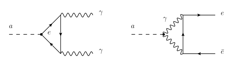
The generated ALP-electron coupling is given as DiLuzio:2020wdo; Georgi:1986df; Srednicki:1985xd; Chang:1993gm; Bauer:2017ris:

where the value of $f_{a}/m_{e}$ is obtained by running the renormalization group from the PQ scale to the scale of the electron mass, with $g^{0}_{a\bar{e}e}=0$ for no tree-level contribution. $g(\tau_{e})$ is the finite loop term with photon coupling as the right handed of figure 1. $g(\tau_{e})$ will expressed as follows Bauer:2017ris:

when $m^{2}_{a}\gg m^{2}_{e}$, $\mathcal{O}\left(\frac{m^{2}_{e}}{m^{2}_{a}}\right)$ approaches to zero. Contributions to the effective coupling $g^{\text{eff}}_{a\bar{e}e}$ can also come from $F\tilde{Z}$ and $Z\tilde{Z}$, but their effects are only significant for larger values of $f_{a}$ and $m_{a}$, which fall outside the scope of this study. Furthermore, as shown in figure 3, any modifications due to these contributions are limited to a maximum of approximately 25%. As the dominant contribution to $g^{\text{eff}}_{a\bar{e}e}$ comes from $g^{\text{eff}}_{a\gamma\gamma}$, we will disregard these other contributions in our subsequent discussion to maintain a simple relation between the two couplings.

Therefore, we have the ratio between the effective ALP-photon and the effective ALP-electron coupling follows the relation without factor $E$,

where $|g^{\text{eff}}_{a\bar{e}e}|$ is naturally smaller due to the loop suppression. In this model, the new physics degree of freedom at low energy is ALP only, because the radial mode of $\Phi$ and vector-like fermion $\mathcal{Q}$ are quite heavy. Therefore, one can focus on the ALP phenomenology and neglect the possible effects from other particles.

Another intriguing ultraviolet model for the invisible QCD axion is the well-known DFSZ model Zhitnitsky:1980tq; Dine:1981rt; Sun:2020iim, where a new Higgs doublet is involved. Unlike usual DFSZ model, our model based on the lepton-specific setup of 2HDM or termed type-X 2HDM Grossman:1994jb; Akeroyd:1994ga; Akeroyd:1996he; Aoki:2009ha; Branco:2011iw; Bhattacharyya:2015nca; Liu:2018xkx. The model consists of two scalar fields, $H_{u}\sim(1,2,1/2)$ and $H_{d}\sim(1,2,1/2)$, which are SU$(3)_{c}$ singlets and SU$(2)_{L}$ doublets, respectively. In addition, the model contains a SM gauge singlet complex scalar $\Phi$, similar as KSVZ model. We write them as:

Moreover, we assign PQ charges to these scalar fields that $X_{1}=-1$, $X_{2}=+1$, and $X_{s}=-X_{1}+X_{2}=+2$, respectively. There are two pseudoscalar Goldstone bosons corresponding to broken $SU(2)_{Y}\times U(1)_{Y}\times U(1)_{PQ}\to U(1)_{EM}$. In the interacting-eigenstates basis $(a_{1},a_{2},a_{s})$, the Goldstone $G_{z}$ eaten by vector gauge boson $Z$ is $(v_{1},v_{2},0)$, and Goldstone $G_{A}$ corresponding to breaking $U(1)_{PQ}$ is $(X_{1}v_{1},X_{2}v_{2},X_{s}v_{s})$. The physical axion $a$ will be a linear combination between $G_{z}$ and $G_{A}$ with $a=c_{1}G_{z}+c_{2}G_{A}$ and $a\cdot G_{z}=0$ Sun:2020iim:

where $v_{\text{SM}}=\sqrt{v_{1}^{2}+v_{2}^{2}}$. So we get the linear combination of the physical states are

where $A_{0}$ is the CP-odd heavy Higgs in the 2HDM.

We assign PQ charge to quarks of $X_{u_{R}}=-1$, $X_{d_{R}}=+1$ and $X_{e_{R}}=-1$, so the Yukawa interactions are

that in our lepton specific setup $H_{d}$ only couples to leptons and $\tilde{H}_{u}=i\sigma_{2}{H_{u}}^{*}$. We will take the SM lepton to be $e$, $e,\mu$ and $e,\mu,\tau$ for three different cases which are denoted as DFSZ-like $(e)$, $(e,\mu)$ and $(e,\mu,\tau)$ respectively. Quarks couple only to $H_{u}$ to obtain the mass. We can get the axion-fermion interaction as

where $m_{u}=\frac{1}{\sqrt{2}}Y_{u}v_{1}$, $m_{d}=\frac{1}{\sqrt{2}}Y_{d}v_{1}$, $m_{e}=\frac{1}{\sqrt{2}}Y_{e}v_{2}$ and $\tan\beta\equiv v_{1}/v_{2}$. The broken scale $f_{a}$ is defined by

where $N_{g}=3$ is the generation number. We note the ratio between the coupling with quarks and the coupling with leptons is $1/\tan^{2}\beta$, thus one can tune the coupling strength between quarks and leptons via $\tan\beta$. After performing the chiral rotation, the $U(1)_{\text{EM}}$ axial anomaly leads to the appearance of the $F\tilde{F}$ term. The $\gamma_{5}$ term $im_{f}\bar{f}\gamma_{5}f$ in eq. (35) can then be expressed as follows Bauer:2017ris; Bauer:2021mvw:

where $c_{u}=-c_{d}=\frac{1}{3}\cos^{2}\beta$ and $c_{\ell}=\frac{1}{3}\sin^{2}\beta$.

$N^{q}_{c}$ is the number of colour (3 for quarks and 1 for leptons), $N_{g}$ is the number of generation and $Q_{i},i=u,d,\ell$ are the electric charges for quarks and leptons respectively. The anomaly coefficient ($E$) will be the second term of eq. 37, that $E=N_{g}(N^{q}_{c}Q^{2}_{u}c_{u}+N^{q}_{c}Q^{2}_{d}c_{d}+N^{e}_{c}Q^{2}_{\ell}c_{\ell})=1$ in the lepton-specific DFSZ-like model. On the other hand, the axial anomaly for SU(3)_C is

with $T(q)=1/2$ (the index of the fundamental representation of SU(3)_C) and the sum ($c_{u}+c_{d}$) being zero implies that the strong CP problem cannot be resolved, because the color anomaly coefficient ($N$) for $G\tilde{G}$ term is 0. Therefore, the lepton-specific DFSZ-like model can only work as an ALP model.

The convention of $c_{u}/f_{a},c_{d}/f_{a}$ and $c_{\ell}/f_{a}$ can be expressed as $g^{\text{eff}}_{a\bar{q}{q}}$, $-g^{\text{eff}}_{a\bar{q}{q}}$ and $g^{\text{eff}}_{a\bar{\ell}\ell}$ respectively. Thus, eq. (37) could be rewritten as follows:

In the lepton-specific DFSZ-like model, the effective ALP-photon coupling comes from the chiral anomaly and also can arise from the ALP-fermion coupling at 1-loop, as shown in the left panel of figure 1. The 1-loop contribution for $g_{a\gamma\gamma}^{\text{1-loop}}$ is Bauer:2017ris; Spira:1995rr

where $f=u,d,\ell$ and $B(\tau_{f})$ are the loop functions given in eq. (3.2). Therefore, adding the tree-level and 1-loop contribution together, the effective ALP-photon coupling can be expressed as follows:

where $B(\tau_{f})$ is expressed as follows:

where $f$ are the SM fermions. The loop functions have two useful limits that,

Therefore, for $m_{f}\gg m_{a}$ the 1-loop contribution for ALP-photon couplings are suppressed, but are comparable to chiral rotation contributions for $m_{f}\lesssim m_{a}$.

In this study, we are going to focus on the ALP-lepton couplings. Contribution to ALP-photon couplings with leptons only are in the same level with both quarks and leptons in the regime of large $\tan\beta$ where $v_{1}\gg v_{2}$. Numerically, we found that for $\tan\beta>10$, the contributions from all fermions and leptons only are of similar magnitude where we show their ratio in figure 2. In the general DFSZ model, the values of $\tan\beta$ are constrained by the perturbative unitarity bound, which lies between 0.25 and 170 DiLuzio:2020wdo; Bjorkeroth:2019jtx; DiLuzio:2016sur; DiLuzio:2017chi. Therefore, we choose $\tan\beta>10$ in this study and neglect the ALP-quark couplings and its contribution to ALP-photon coupling. This is a good approximation for examining the concurrence features of ALP-photon coupling and ALP-electron coupling. Other physical scalars are quite heavy to avoid phenomenological constraints, thus the lower-energy phenomenon are the physical ALP in the scalar sector. We take the ratio between the electron-ALP coupling ($g^{\text{eff}}_{a\bar{e}e}$) and photon-ALP coupling with leptons only ($g^{\text{eff}}_{a\gamma\gamma}$), and the expression is

Since we have the same $g^{\text{eff}}_{a\bar{\ell}\ell}$ for all three leptons, the ratio above can be simplified as $|\frac{\alpha_{\text{QED}}}{4\pi}\sum_{\ell=e,\mu,\tau}\left(B(\tau_{f})-1\right)|$. If the ALP only couples to electrons, the ratio factor can be simplified to $\frac{\alpha_{\text{QED}}}{4\pi}\left(B(\tau_{e})-1\right)$. Therefore, the ratio factor serves as an effective model constraint when considering the concurrent effects of two couplings. For our analysis, we adopt $m_{e}=0.000511$ GeV, $m_{\mu}=0.1056$ GeV, and $m_{\tau}=1.78$ GeV.

This section discusses the decay properties of ALP with respect to electrons $|g^{\text{eff}}_{a\bar{e}e}|$ and photons $|g^{\text{eff}}_{a\gamma\gamma}|$, and their characteristics in the context of the aforementioned ultraviolet models. The combined effects of these two couplings and the mass of ALP $m_{a}$ result in an increased decay width of the ALP and are crucial for determining the branching ratios. In figure 3, the ratio $|g^{\text{eff}}_{a\gamma\gamma}|/|g^{\text{eff}}_{a\bar{e}e}|$ from two ultraviolet models are plotted as a function of $f_{a}$ for four values of $m_{a}$: 0.002, 0.02, 0.5, and 5 GeV, from top left to bottom right. The KSVZ-like model ratio (purple line) follows eq. (18). The DFSZ-like model ratio follows eq. (46), represented by three black lines in the figure (the solid line corresponds to only $e$ in the fermion loop, the dotted line includes $e$ and $\mu$, and the dashed line consists of all three leptons, $e$, $\mu$, and $\tau$). The ratio of the DFSZ-like model is independent of $f_{a}$ because the coupling decay constants $f_{a}$ are cancelled out, while the KSVZ model is dependent and correlated with two parameters, $m_{a}$ and $f_{a}$. Due to the modulus of real and imaginary contribution, the maximum ratio would vary with values of $f_{a}$ and ranges from $10^{0.5}$ to $10^{2}$ for $f_{a}$ from $10^{0}$ to $10^{20}$ GeV, which changes very mild due to logarithmic dependence. The values of the ratio between the two couplings in the KSVZ-like model are consistently greater than those in the DFSZ-like model for all four choices of $m_{a}$. This disparity can be attributed to the presence of the correlation factor $\alpha_{\text{QED}}$ within the effective ALP-electron coupling, as described by eq. (16). This factor enhances the ratio by reducing the denominator to a significantly smaller value, resulting in a stronger preference for ALP-photon coupling in the KSVZ-like model.

In figure 4, we show four plots with BR($a\to\gamma\gamma$) (solid blue for 99.8%, solid green for 50% and solid orange for 0.2%) in the $\{|g^{\text{eff}}_{a\bar{e}e}|,|g^{\text{eff}}_{a\gamma\gamma}|\}$ 2D plane with $m_{a}$ equals to 0.002 GeV (top left panel), 0.01 GeV (top right panel), 0.5 GeV (bottom left panel) and 2 GeV (bottom right panel) respectively. The decay branching ratio to electrons, BR($a\to\bar{e}e$), on the other hand, will then equal $1$ - BR($a\to\gamma\gamma$). We illustrated the ultraviolet models, represented by the purple band for KSVZ-like and black lines (solid for $e$ contribution only, dotted for $e,\mu$ contributions, and dashed for all three lepton, $e,\mu,\tau$ contributions) for DFSZ-like. We found that BR($a\to\gamma\gamma$) is dominant when both $g^{\text{eff}}_{a\gamma\gamma}$ and $g^{\text{eff}}_{a\bar{e}e}$ couplings are in the same order for heavier $m_{a}$ states (see plots with $m_{a}=$ 0.5 and 2 GeV). Conversely, when $m_{a}$ decreases, BR($a\to\bar{e}e$) increases because that the decay ratio between $a\to\gamma\gamma$ and $a\to\bar{e}e$ is directly proportional to $m^{2}_{a}/8m^{2}_{e}$. Therefore, these decay properties can be combined with existing experimental results to provide testable predictions.

For the constraint on the ALP-photon coupling, the limit from the Belle-II experiment Belle-II:2020jti is considered. This limit covers the ALP mass detection range between 0.2 and 9.7 GeV from electron-positron collisions ($e^{+}+e^{-}\to\gamma+a$) followed by $a\to\gamma\gamma$, with three photons in the final state. The data was collected with an integrated luminosity of 445 pb^-1 at the center-of-mass energy of $\sqrt{s}=10.58$ GeV. The background is dominated by $e^{+}e^{-}\to e^{+}e^{-}(\gamma)/,\gamma\gamma(\gamma)$ and pseudoscalar meson processes, such as $\pi^{0},\eta,\eta^{\prime}$ with $\gamma$ in the final state. For ALP-electron coupling constraint, the exclusion limit comes from BaBar Batell:2009yf; BaBar:2014zli; Bauer:2017ris; Bauer:2018uxu in the mass region roughly between 0.02 and 9.2 GeV. The data collection has been performed within a luminosity of 514 fb^-1 at $\Upsilon(2S,3S,4S)$ resonance. The background events were simulated similarly to the Belle-II search, while BaBar used electron-positron collisions with two leptons and one photon as the final products.

The tree-level Feynman diagrams in figure 5 are associate ALPs production with ALP-photon and ALP-electron couplings in the collider searches. The analytical formula for the cross-section of $e^{+}e^{-}\to a\gamma$ can be obtained by integrating the differential cross-section concerning the scattering angle, as calculated using the programs FeynRules 2.0 Alloul:2013bka, and FeynCalc 9.3 Mertig:1990an; Shtabovenko:2016sxi; Shtabovenko:2020gxv with patched FeynArts 3.11 Hahn:2000kx, and it can be expanded using small $m_{e}$ as follows,

The first term in the first line, $(g^{\text{eff}}_{a\gamma\gamma})^{2}$ term in eq. (47), is the main term for the ALP-photon coupling in the $e^{+}e^{-}\to a\gamma$ cross-section process which corresponds to the $s-$channel diagram in the left panel of figure 5. If $g^{\text{eff}}_{a\gamma\gamma}$ and $g^{\text{eff}}_{a\bar{e}e}$ are similar in magnitude, the ALP-photon coupling has a greater impact on the cross-section for low $m_{a}$ values, and it is because the interference term $g^{\text{eff}}_{a\gamma\gamma}g^{\text{eff}}_{a\bar{e}e}$ and ($g^{\text{eff}}_{a\bar{e}e}$)² is suppressed by $m^{2}_{e}/s$.

The constraints set by the Belle-II Belle-II:2020jti and BaBar BaBar:2014zli searches covering single coupling, can be adapted to our concurrent scenario. In the left panel of figure 6, we depict the $\sigma(g^{\text{eff}}_{a\bar{e}e},g^{\text{eff}}_{a\gamma\gamma})_{\text{int}}/\sigma(g^{\text{eff}}_{a\bar{e}e},g^{\text{eff}}_{a\gamma\gamma})$ ratio, where the numerator is the interference contribution in the cross-section and the denominator is the full cross-section. One can see that the ratio is as small as $\mathcal{O}(10^{-4})$, that the interference effect is negligible due to the $m_{e}^{2}g^{\text{eff}}_{a\bar{e}e}/(sg^{\text{eff}}_{a\gamma\gamma})$ factor. In addition, we plot the contours of cross-section $\sigma$ equal to BaBar (solid blue) and Belle-II (solid red) limits to illustrate the excluded region in the 2D plane $[|g^{\text{eff}}_{a\bar{e}e}|,|g^{\text{eff}}_{a\gamma\gamma}|]$ at $m_{a}=0.5$ GeV. For comparison, we have plotted the exclusion limits from previous experiments for single coupling scenario, indicated by the light blue and orange dashed lines for BaBar and Belle-II respectively. The regions on the upper-right side of solid curves would be ruled out. Compared to single coupling scenario, more regions are ruled out due to larger cross-section induced by concurrent couplings, for example, some areas on the left-hand side of the light blue dashed line.

To examine the cross-section of electron-positron annihilation with the ALP followed by di-electron and diphoton decay channels, we analyze the ALP final states for the existing limits by multiplying $\sigma(e^{+}+e^{-}\to a+\gamma)$ with BR($a\to\bar{e}e/\gamma\gamma$). In the right panel of figure 6, with same benchmark point of $m_{a}=0.5$ GeV, the product $\sigma\times$ BR($a\to\bar{e}e/\gamma\gamma$) (light blue / orange exclusion regions) are plotted and only white area is allowed by experiments. The concurrent effect is induced by two factors. One is cross-section which reduces the allowed parameter space, and another is the branching ratio (BR), which in contrast, tends to relax constraints. For BaBar limits, We know from the left panel that bending from vertical to left is attributed to larger cross-section after considering $g_{a\gamma\gamma}^{\text{eff}}$, while bending from left to up is due to BR effect. Specifically, the region with $|g^{\text{eff}}_{a\bar{e}e}|<$ 10^-2 GeV^-1 and $|g^{\text{eff}}_{a\gamma\gamma}|>$ 10^-4.5 GeV^-1 evades the BaBar limit ($\sigma_{\text{BaBar}}$ on the left panel excludes $|g^{\text{eff}}_{a\bar{e}e}|>$ 10^-1.5 GeV^-1 and $|g^{\text{eff}}_{a\gamma\gamma}|>$ 10^-4.5 GeV^-1) because a large effective coupling $|g^{\text{eff}}_{a\gamma\gamma}|$ decreases the branching ratio BR($a\to\bar{e}e$), thereby suppressing the product of the cross-section and branching ratio ($\sigma$BR). For Belle-II limits, the open areas with $|g^{\text{eff}}_{a\bar{e}e}|>$ 10^-1 GeV^-1 and 10${}^{-3}<|g^{\text{eff}}_{a\gamma\gamma}|<10^{-2.5}$ GeV^-1 relax the bound by the suppression of BR($a\to\bar{e}e$).

In the right panel of figure 6, we have incorporated UV model suggested parameter space from the modified DFSZ-like model with diagonal black lines (solid, dotted and dashed) and the KSVZ-like model with two purple lines (solid and dashed) corresponding to $f_{a}=10^{3}$ GeV and $f_{a}=10^{12}$ GeV, respectively. For $m_{a}=0.3$ GeV, the KSVZ-like model is fully excluded in the 2D plane, while the DFSZ-like model are still survived for coupling to $(e,\mu)$ and $(e,\mu,\tau)$ but the electron only coupling is excluded.

We consider more ALP masses, $m_{a}=1$ GeV and $m_{a}=5$ GeV, in the left and right panels of figure 7. The figure for $m_{a}=1$ GeV is qualitatively similar to $m_{a}=0.5$ GeV, but the allowed region expands. For $m_{a}=5$ GeV, comparing with the single coupling scenario, the BaBar constraint becomes weaker, while Belle-II becomes stronger, opposite to the situation of smaller ALP masses. These differences in different mass comes from the fact that BR$(a\to\gamma\gamma)$/BR$(a\to e\bar{e})$ is propotional to $m_{a}^{2}$. Therefore, for larger $m_{a}$, the BR$(a\to\gamma\gamma)$ enhances the product $\sigma$BR and surpass the existing Belle-II limit. In contrast, the allowed region for BaBar is increased due to suppression of BR($a\to\bar{e}e$).

ALPs can be searched using electron and positron colliders, especially for masses around $\mathcal{O}(1\sim 10)$ GeV. However, for lighter ALPs beam dump experiments are cost-effective, since the fixed target or beam dump experiments can provide higher luminosity than colliders. Specifically, beam dump experiments have a low-energy configuration that allows for the effective searches of ALPs with lower masses, ranging from 1 MeV to roughly 1 GeV. In general, electron, muon and proton beams can be used for beamdump searches. In this study, we focus on electron beamdump searches for our purpose of investigating the concurrence scenario of both $g_{a\bar{e}e}^{\text{eff}}$ and $g_{a\gamma\gamma}^{\text{eff}}$ couplings.

In table 1, several constraints established through the electron beamdump method have been listed, along with their experimental setups. Searches such as KEK Ishikawa:2021qna, E141 Riordan:1987aw, E774 Bross:1989mp and Orsay Davier:1989wz used Tungsten (W) as target materials while the dominant exclusion limits E137 Bjorken:1988as; Liu:2017htz and NA64 NA64:2020qwq; Dusaev:2020gxi; NA64:2021aiq used Aluminium(Al) and Lead(Pb) respectively. Constraints have been set using E137 on ALP-electron coupling Bjorken:1988as; Liu:2017htz and ALP-photon coupling Essig:2010gu; Bjorken:1988as, and have been set using NA64 on ALP-photon coupling NA64:2020qwq; Dusaev:2020gxi and ALP-electron coupling NA64:2021aiq, but these limits are all considered in single coupling scenario. Therefore, in this study, we recast the ALP limits of E137 and NA64 experiments under the concurrence of the ALP-electron and ALP-photon couplings.

Both E137 and NA64 constraints consider ALPs produced by incident GeV-electron beam on target, where the ALPs penetrate through shield and decay into electron pairs or photon pairs. The sensitivity of E137 was obtained from the production of pseudoscalar particles where a 20 GeV electron beam was directed at an Aluminium target, penetrating a 179 m long shield and decaying in the 204 m length detector. On the other hand, NA64 experiment utilized a 100 GeV electron beam, passed through one 0.45 m ECAL (Electromagnetic Calorimeter) module, and three 1.3m HCAL (Hadron Calorimeter) modules in the lead target sector. It has two different experimental setups NA64:2021aiq and we use the ”invisible mode” configuration where the ECAL serves as the target and one HCAL serves as the shield. This configuration still has two search strategies, one for visible signature that ALPs decay in the latter two HCAL modules, while another for invisible signature that the decay position of ALP is assumed to be at the end of the detector (after ECAL and HCAL modules). In our analysis, we consider limits from invisible signature of NA64 and it is in good accordance with the limits which is set under the scenario of single coupling between ALP and electron or photon.

To estimate the number of detectable ALPs in beam dump experiments, we need to tackle the cross-section of the 2 to 3 production process first: $e^{-}N\to e^{-}aN$, where ALP is produced from the collision of incoming electrons with fixed target materials, and this can be done by utilizing the Improved Weizsäcker-Williams (IWW) approximation method. The concept behind this approach was to simplify the cross section calculation for a 2 to 3 process by reducing it to a 2 to 2 process, simplifying phase space integral. The idea is that the virtual photon emitted from the nuclei can be seemed as real photons under this approximation. This was done to decrease the computational complexity, but it would require mass of the new particle to be significantly smaller than the energy of the incoming beam and result a highly collinear final states. More detailed explanations can be found in refs. Tsai:1966js; Kim:1973he; Tsai:1973py; Tsai:1986tx; Bauer:2018onh. The Feynman diagrams for the simplified 2 to 2 ALP production are depicted in the middle panel of figure 8. One contribution comes from the Primakoff-like process (the middle panel) via ALP-photon coupling, and there are also contributions from dark bremsstrahlung process (the left and right panels) via ALP-electron coupling.

With IWW approximation, the fraction of cross-section distribution over the energy transfer ratio ($x=E_{a}/E$) is represented by Tsai:1966js; Liu:2017htz:

where $E$ is the energy of initial-state electrons, $\mathcal{A}$ is the approximate 2 to 2 amplitude and $\chi$ is an effective flux of photons Gninenko:2017yus