Solving the domain wall problem with first-order phase transition

Yang Li Affiliation: School of Physical Sciences, University of Chinese Academy of Sciences, No. 19A Yuquan Road, Beijing 100049, China Affiliation: CAS Key Laboratory of Theoretical Physics, Institute of Theoretical Physics, Chinese Academy of Sciences, P.O. Box 2735, Beijing 100190, China Ligong Bian Email: lgbycl@cqu.edu.cn Affiliation: Department of Physics and Chongqing Key Laboratory for Strongly Coupled Physics, Chongqing University, Chongqing 401331, P. R. China Affiliation: Center for High Energy Physics, Peking University, Beijing 100871, China Yongtao Jia Affiliation: Department of Physics and Chongqing Key Laboratory for Strongly Coupled Physics, Chongqing University, Chongqing 401331, P. R. China

Abstract

Domain wall networks are two-dimensional topological defects generally predicted in many beyond standard model physics. In this Letter, we propose to solve the domain wall problem with the first-order phase transition. We numerically study the phase transition dynamics, and for the first time show that the domain walls reached scaling regime can be diluted through the interaction with vacuum bubbles during the first-order phase transition. We find that the amplitude of the gravitational waves produced by the second-stage first-order phase transition is several orders higher than that from the domain walls evolution in the scaling regime. The scale of the first-order phase transition that dilute the domain walls can be probed through gravitational waves detection.

Introduction. Domain walls (DWs) are two-dimensional surface-like topological defects forming after the spontaneous breakdown of a discrete symmetry in the early Universe Kibble 1976; Zurek 1985; Zeldovich et al. 1974. DWs are generally predicted in many particle physics models, such as axion models Sikivie 1982a; Vilenkin and Everett 1982; Hiramatsu et al. 2011; Hiramatsu et al. 2013; Kawasaki et al. 2015, supersymmetric models Abel et al. 1995; Takahashi et al. 2008; Dine et al. 2010; Hamaguchi et al. 2012; Kadota et al. 2015, thermal inflation Moroi and Nakayama 2011, etc. If the domain wall networks are stable they would eventually overclose the universe and therefore conflict with the present cosmological observations, since the energy density of DWs decreases slower than that of matters and radiations, this is the well-known domain wall problem Zeldovich et al. 1974. The conventional way to resolve this problem is to introduce a biased potential to lift the degenerate minima so that the walls will annihilate at sufficiently early times Coulson et al. 1996; Gelmini et al. 1989; Vilenkin 1981; Larsson et al. 1997; Sikivie 1982b and remains the stochastic gravitational wave background (SGWB)Gleiser and Roberts 1998; Hiramatsu et al. 2010; Kawasaki and Saikawa 2011; Hiramatsu et al. 2014. More recently, the PPTA and NANOGrav datasets are used to place constraints on the SGWB produced emitted by DW networks Bian et al. 2022; Ferreira et al. 2023.

In this Letter, we propose to evade the domain wall problem with the following first-order phase transition (PT) process after the DWs are formed. Recent development of gravitational wave (GW) astronomy provides a distinctive way to probe particle physics predicting first-order PT in the early Universe Caprini et al. 2016; Bian et al. 2021a; Caprini et al. 2020; Cai et al. 2017; Caldwell et al. 2022. Recent constraints on the low-scale phase transitions are placed with the dataset of Parkes Pulsar Timing Array (PPTA) and NANOGrav collabrations Bian et al. 2021b; Xue et al. 2021; Arzoumanian et al. 2021. The first constraints on the PeV-EeV scale phase transitions are reached in Ref. Romero et al. 2021 by utilizing the data from the third observing runs of LIGO-Virgo.

In particular, we will focus on two-step PTs where the DW defects are created in the first step and the first-order PT happens in the second step. Both the first-step second-order PT together with DWs evolution and the second-step first-order PT are expected to generate GWs. When DWs are formed after the first-step second order PT, they would evolve toward the “scaling regime” where the typical length scales of the DWs network ( the curvature radius and the distance between neighboring DWs) become comparable to the Hubble radius ( $H^{-1}$ ). In this regime, DWs would frequently interact with each other, changing their configuration or collapsing into the closed walls to maintain the scaling property, and yields GW generation Hiramatsu et al. 2010; Kawasaki and Saikawa 2011; Hiramatsu et al. 2014. The scenario where the first-order PT leads to the breakdown of the electroweak symmetry is well motivated for dark matter and baryon asymmetry of the UniverseMcDonald 1994; Burgess et al. 2001; Espinosa and Quiros 2007; Profumo et al. 2007; Barger et al. 2008; Espinosa et al. 2008; Espinosa et al. 2012a; Espinosa et al. 2012b; Cline and Kainulainen 2013; Profumo et al. 2015; Feng et al. 2015; Curtin et al. 2014; Craig et al. 2016; Huang et al. 2016; Vaskonen 2017; Curtin et al. 2018; Kurup and Perelstein 2017; Buttazzo et al. 2018; Caprini et al. 2020; Alanne et al. 2020; Costantini et al. 2020; Al Ali et al. 2022.

We numerically study the formation and decay of the DWs followed by a first-order PT, and find that vacuum bubbles would expand and collide with each other and DWs. We characterize the DWs behavior with scaling parameters by including the interplay between vacuum bubbles and DWs for the first time. The scaling parameter of DWs indicates that the DWs decay is a natural result of the collision between DW networks and vacuum bubbles during the second stage. After vacuum bubbles are generated, vacuum bubbles would expand and collide with each other and domain walls to generate GWs. We also find that the first-order PTs dominate the amplitude and shape of the GW spectrum.

The model. For simplicity and without loss of universality, we consider the domain walls being formed after spontaneous symmetry breaking of a $Z_{2}$ symmetry, and the second step is a first-order phase transition to restore the $Z_{2}$ symmetry. With the high-temperature approximation, the thermal potential keeping only the terms up to $\propto T^{2}$ is given by,

	$\displaystyle V(S,h)$	$\displaystyle=$	$\displaystyle-\frac{1}{2}(av^{2}-c_{h}T^{2})h^{2}+\frac{\lambda_{h}}{4}h^{4}$		(1)
			$\displaystyle-\frac{1}{2}(bv^{2}-c_{S}T^{2})s^{2}+\frac{\lambda_{S}}{4}s^{4}+\frac{\lambda_{Sh}}{2}h^{2}s^{2},$		(1)

with $\lambda_{Sh,S,h}>0$ , and $v$ being a scale parameter. For the case where the second step is a spontaneous EW symmetry-breaking process, one has $av^{2}=\mu_{h}^{2},bv^{2}=\mu_{S}^{2}$ , and the thermal effects are captured by $c_{h}$ and $c_{s}$ Espinosa et al. 2012a:

c_{h}=\frac{2m_{W}^{2}+m_{Z}^{2}+m_{h}^{2}+2m_{t}^{2}}{4v^{2}}+\frac{\lambda_{Sh}}{12},\quad c_{S}=\frac{4\lambda_{Sh}+3\lambda_{S}}{12},

(2)

With the thermal potential, all symmetries are restored at high temperatures. As the Universe cools down, the discrete $Z_{2}$ symmetry firstly breakdown spontaneously with the singlet scalar $S$ developing a non-vanishing vacuum expectation value $\langle S\rangle=\pm v_{s}=\pm\mu_{S}/\sqrt{\lambda_{S}}$ , with the space regions equivalently fails into $+$ and $-$ domains formed inside a Hubble patch separated by domain walls at the boundaries: $S_{\text{DW}}(z)=v_{s}\,\text{tanh}(\mu_{S}z/\sqrt{2})$ . Later, the DWs would enter into the scaling regime or not depending on if the time separation between the first-step and the second-step PTs is long enough. Then, the first-step PT occurs equivalently either inside the $+$ or $-$ domains, with the vacua of $(\langle h\rangle,\langle S\rangle)$ transiting as $(0,\pm v_{s})\rightarrow(v_{h}=\mu_{h}/\sqrt{\lambda_{h}},0)$ . Since we intend to study the dynamics from the formation of domains walls and the effects of the first order PT on the evolution of DWs network, we do not consider bias term to appear as in Ref. McDonald 1995; Espinosa et al. 2012b. For the study of the seeded vacuum decay by domain walls, we refer to Ref. Blasi and Mariotti 2022; Blasi et al. 2023, where the formed domain walls are required not to collapse before the second-step PT has been completed. We note that to obtain the desired phase transition the following two requirements are necessary Bian and Tang 2018: 1) at zero temperature, the local vacuum at $(h,S)=(0,\pm v_{S})$ should be higher the global one at $(h,S)=(v_{h},0)$ , which yields $\lambda_{S}\lambda_{h}>2\mu_{S}^{4}/(2\mu_{h}^{4})$ with $\mu_{h}^{2},\mu_{S}^{2}>0$ ; and 2) the first step second-order phase transition occurs earlier than the second-step first-order phase transition: $\mu_{h}^{2}/c_{h}<\mu_{S}^{2}/c_{S}$ .

The simulation framework. At high temperatures before the phase transition occurs in the radiation-dominant universe, we consider the scalar field $S$ evolving from their initial thermal configuration until the critical temperature when the second-order PT occurs, and the amplitude and momentum of the field $h$ initially have vanishing values. As the temperature future cools down, the quantum tunneling process realizes through vacuum bubbles nucleation in the second-step first-order PT. During the numerical simulation of the classical scalar fields, the transverse-traceless(TT) part of the anisotropic energy-momentum tensor ( $\Pi^{TT}_{ij}=(\partial_{i}s\partial_{j}s+\partial_{i}h\partial_{j}h)$ ) would induce the spatial metric perturbations $h_{ij}$ and contribute to GWs energy density $\rho_{gw}=\langle\dot{h}_{ij}(x,t)\dot{h}_{ij}(x,t)\rangle_{V}$ with $\langle...\rangle_{V}$ denoting spatial average over the whole simulation volume. To eliminate the influence of the initial conditions (especially different initial temperatures) on the GWs power spectrum, we start to evolve the spatial metric perturbations ( $h_{ij}$ ) from the critical temperature of the second-orderPT (see Supplemental material for details).

We intend to study the case where DWs reach the scaling regime before the first-order PT, and the parameters in the thermal potential are chosen as follows: $\lambda_{h}=0.129$ , $\lambda_{Sh}=0.66$ , $\lambda_{S}=1$ , $a=0.781$ , $c_{h}=0.4534$ , $b=1.104$ , $c_{S}=0.235$ . Therefore, the critical temperature of second-order PT is about $T_{\rm c}=2.17v$ . For the convenience of numerical simulation, all scalar fields $(S,h)$ are rescaled with the scale parameter $v$ , and the grid size $dx$ (and time-step) are rescaled by $w_{*}=a_{i}H_{i}$ with the $a_{i}$ and $H_{i}$ being initial scale factor and Hubble parameter. It is convenient to take the rescaled conformal time $\tilde{\eta}(=\eta/\eta_{i})$ with the initial conformal time being $\eta_{i}=1/w_{*}$ in our simulations. We fix $\tilde{\eta}=1$ to be the initial time at which $T=12T_{\rm c}$ , so the second-order PT happens at $\tilde{\eta}=12$ . We set $v=6\times 10^{16}{\rm GeV}$ to ensure the simulation box can capture large enough Hubble volume and have enough time to evolve the DWs network.

We use the second-order leap-frog algorithm adopted by ${\mathcal{C}osmoLattice}$ Figueroa et al. 2023; Figueroa et al. 2021 to evolve the equations of motion in a simulation box of comoving side-length $L=190/(a_{i}H_{i})$ and $N=1024$ points per side. So, the dimensionless comoving lattice spacing is about $\delta\tilde{x}=0.19$ , and the dimensionless time-step is chosen as $\delta\tilde{\eta}=0.005$ . As the temperature decreases to about $T=0.5v$ ( $\tilde{\eta}=52.38$ ) when the domain walls have entered the scaling regime, the quantum tunneling process of the first-order PT occurs, the bubble profile functions of $s$ and $h$ fields have the following form

	$\displaystyle s(r)_{\pm}=\pm 0.7v\pm\frac{s_{v}}{2}\left(1+{\rm tanh}\left[\frac{r-(R_{\rm in}+0.5L_{\rm w})}{L_{\rm w}}\right]\right),$		(3)
	$\displaystyle h(r)=\frac{h_{v}}{2}\left(1-{\rm tanh}\left[\frac{r-(R_{\rm in}+0.5L_{\rm w})}{L_{\rm w}}\right]\right),$		(4)

where $s_{v}=0.32v$ , $h_{v}=1.1v$ , $r\in[0,25]\delta x_{\rm phy}$ , $R_{\rm in}=10\delta x_{\rm phy}$ , $L_{\rm w}=12\delta x_{\rm phy}$ , $\delta x_{\rm phy}$ is the physical lattice spacing when bubble is generated. The PT strength (the latent heat normalized by the radiation energy) can be estimated to be $\alpha=(V(0,\langle s\rangle)-V(\langle h\rangle,0))/\rho_{r}\approx 0.276$ . We randomly generate bubbles far from the DWs. For our simulation, the vacuum bubbles can be considered to generate simultaneously with the bubble nucleation rate $\beta\approx 8\pi(N_{b}/\mathcal{V})^{1/3}$ with the $N_{b}$ and $\mathcal{V}$ being bubbles number and the volume of the simulation box Hindmarsh et al. 2021. We place the different number of bubbles in the simulation box to study the effect of the number of bubbles (denote as $N_{\rm b}$ ) on the simulation, i.e. $N_{\rm b}$ =512 and $N_{\rm b}$ =64 in the physical volume of $V=48H_{PT}^{-3}$ which correspond to the inverse PT durations being $\beta/H_{PT}=55.3$ and $27.7$ . For concreteness, we use $s(r)_{+}$ to generate bubbles for the field $s$ in the spherical region where the average value of $s$ is greater than 0.9 $v$ , and use $s(r)_{-}$ to generate bubbles for the field $s$ in the spherical region where the average value of $s$ is smaller than $-0.9v$ . In each spherical region that the $s$ field generates bubbles with $s(r)_{+}$ or $s(r)_{-}$ , we use the $h(r)$ profile function to generate bubbles for the field $h$ . We evolve the equations of motion until the final time $\tilde{\eta}=150$ . At this time, the simulation box contains about two Hubble volumes to reduce finite volume effects, and the thickness of the domain wall is about twice the physical lattice spacing to obtain sufficient resolution.

Refer to caption — Figure 1: Evolutions of the average amplitudes of field $s$ and $h$ for the case of $N_{\rm b}=512$ .

Results. For illustration, in Fig. 1, we present the averaged field values of $h$ and $s$ for the case of $N_{\rm b}=512$ , where we can observe that, as the universe cools down, the average amplitude of the fields $s$ and $h$ changes. The averaged amplitude of $h$ increase when the first-order PT occurs and stay stable when the phase transition is completed, and the averaged amplitude of $s$ drops below zero when the first-order PT start and back to zero when the first-order PT finished associated with the whole volume are full of vacuum: $(\langle h\rangle,\langle s\rangle)=({h_{v},0})$ . The three-dimensional distribution of the DWs of the field $s$ and the bubbles of the field $h$ at different times are shown in Fig. 2, which reflect the physical picture of the PT dynamics. The top-left graph shows that bubbles are randomly generated away from the domain wall. The remaining three graphs show that as bubbles expand, collisions between bubbles and domain walls, as well as collisions between different bubbles cause the domain walls to decay.

To reflect the impact of the number of bubbles on the domain walls’ evolutions, we quantitatively describe the decay process of the DWs by measuring the scaling parameters in three cases( $N_{\rm b}=0,N_{\rm b}=64$ and $N_{\rm b}=512$ ), see Fig. 3. For the case without considering the first-order phase transition, we obtain the scaling parameter $\xi_{\rm dw}\approx 1$ , which is in agreement with previous studies of domain wall dynamics Hiramatsu et al. 2014 except that our simulation time is much longer and the scaling parameter is more stable, see Supplemental material for details. The scaling parameter drops as the first-order PT process proceeds, and the faster PT case with more vacuum bubbles would yield an earlier decrease of the scaling parameter. We refer to the moment when the scaling parameter drops to half of its value in the scaling regime as the decay time of the DW. So, as can be seen from the figure. Combining the three-dimensional shape of the potential and the profile function of the bubbles of the fields $s$ and $h$ , it can be inferred that due to the expansion of the bubbles, the domain wall located in the false vacuum feels the pressure difference with the true vacuum when it collides with the bubble. This pressure difference causes the false vacuum at the domain wall to be pushed to a true vacuum, which causes the decay of the domain wall. As the first-order PT complete, the scaling parameters $\xi_{\rm dec,1}$ and $\xi_{\rm dec,2}$ gradually reach zero.

We show the GW energy density power spectrum of the case of $N_{\rm b}=512$ in Fig. 4. The magnitude of the GWspectrum produced by domain walls at the time of $\tilde{\eta}=30.8$ is found to be around $10^{-6}$ , the amplitude of the gravitational waves spectrum grows by almost four orders with first-order PT process continues and stop grows as the first-order PT complete. In the figure, the four characteristic scales are given: $k_{\rm H}=(2\pi H_{\rm dec})\times a(\tilde{\eta}_{\rm dec})/(a_{i}H_{i}),\quad k_{\rm b}=2\pi/(V/N_{\rm b})^{1/3}/(a_{i}H_{i}),\quad k_{{\rm L}_{\rm w}}=2\pi/L_{\rm w}\times a(\tilde{\eta}_{\rm gen})/(a_{i}H_{i}),\quad k_{\rm dw}=(2\pi/\delta_{\rm dw})\times a(\tilde{\eta}_{\rm sc})/(a_{i}H_{i})$ , which corresponds to the Hubble parameter at the time of the decay of DWs ( $H_{\rm dec}$ ), the DWs decay time( $\tilde{\eta}_{\rm dec}$ =63.81), the mean bubble separation is $R_{\star}=(V/N_{\rm b})^{1/3}$ ( $V$ is the comoving volume of the simulation box, $N_{\rm b}$ is the number of vacuum bubbles) , the wall thickness $L_{\rm w}$ when the bubbles are generated ( $\tilde{\eta}_{\rm gen}$ is the time when bubbles are generated), the physical thickness of the domain wall when just entering the scaling regime ( $\delta_{\rm dw}$ , where $\tilde{\eta}_{\rm sc}$ is the time when domain wall just entering the scaling regime).

The GW energy density of the DWs in the scaling regime would be proportional to the square of DWs surface tension: $\rho^{DW}_{gw}\sim G\mathcal{A}^{2}\sigma_{\rm dw}^{2}$ Hiramatsu et al. 2013, $\sigma_{\rm dw}=(2\sqrt{2}/3)b^{\frac{3}{2}}\lambda_{S}^{-1}v^{3}$ , the area parameter is estimated to be almost $\mathcal{A}\equiv\xi_{\rm dw}=1.09$ in the scaling regime for our simulations. Fig. 5 indicates that the GW spectrum from DWs is found to be almost flat in intermediate frequencies between the scale corresponding to the horizon size at the decay time of DWs ( $k_{H}$ ) and that of the DWs width $k_{\rm dw}$ , this is because the DWs reach scaling regime and stay in the regime for a long while. The GW energy density from bubble collisions during the first-order PT is expected to $\rho^{PT}_{gw}\sim\rho_{c}(H_{PT}/\beta)^{2}(\alpha/(\alpha+1)^{2})$ with the $\rho_{c}$ being the total energy density when the PT occurs Huber and Konstandin 2008; Konstandin 2018. Fig. 5 shows that the amplitude of the GW spectra is much higher when the first-order PT occurs, this is mainly because there are more bubble walls in comparison with DWs in the same Hubble volume. Therefore, the contribution to GWs would be dominated by first-order PT rather than the DW for the scenarios under study. If the DWs annihilation is driven by a much lower scale of first-order PT, one might comparable contributions of $\rho^{PT}_{gw}\sim\rho^{DW}_{gw}$ which yields $G\mathcal{A}^{2}\sigma_{dw}^{2}\sim\left(3H_{PT}^{2}/(8\pi G)\right)(H_{PT}/\beta)^{2}\left(\alpha/(\alpha+1)^{2}\right)$ . We numerically confirm that the case with fewer vacuum bubbles can produce a larger amount of GW radiations since it yields a slower PT with larger $H_{PT}/\beta$ Huber and Konstandin 2008; Di et al. 2021; Zhao et al. 2022; Cutting et al. 2018; Cutting et al. 2021, the ratio of the amplitude of the GWs spectra is numerically checked to be: $\Omega_{GW}(N_{b}=512)/\Omega_{GW}(N_{b}=64)\sim((H_{PT}/\beta)_{N_{b}=64}/(H_{PT}/\beta)_{N_{b}=512})^{2}\sim 4$ . We therefore can expect that the GWs spectrum generated by long-live DWs decay before BBN driven by the bias term as in literatures Hiramatsu et al. 2010; Kawasaki and Saikawa 2011; Hiramatsu et al. 2014 would be pretty different from that driven by the first-order PT. Though we cannot obtain the power-law of $k^{3}$ for the GWs spectra in the IR regions required by the causality due to the limitation of the simulation box, we take $k^{3}$ for the GWs spectra prediction in the following. The power-law on the right-hand side of the peak frequencies of $k_{\rm H}$ and $k_{\rm b}$ are numerically found to be: $\Omega_{GW}^{DW}\propto k^{-2.14}$ and $\Omega_{GW}(N_{b}=64,512)\propto k^{-1.60,-1.09}$ .

For the GWs generation from the DWs evolution in the scaling regime, we have the peak amplitude being $\Omega^{p}_{DW}=8\pi\tilde{\epsilon}_{gw}G^{2}\mathcal{A}^{2}\sigma^{2}/(3H^{2})$ with the efficiency parameter of GWs production being estimated to be $\tilde{\epsilon}_{gw}=0.49$ , see Supplemental material. Considering the GWs production process ended in the radiation dominated Universe, the present GWs amplitude can be obtained as $\Omega^{p}_{DW}h^{2}(t_{0})=1.67\times 10^{-5}(100/g_{\star})^{1/3}\Omega^{p}_{DW}$ with the relativistic degrees of freedom being $g_{\star}=106.5$ Kamionkowski et al. 1994. The present peak frequency determined by the DWs decay before BBN driven by some bias terms can be obtained as Saikawa 2017: $f^{p}_{DW}(t_{0})\approx 1.1\times 10^{-9}{\rm Hz}(g_{\star}(T_{dec})/10)^{1/2}(g_{\star,s}(T_{dec})/10)^{-1/3}(T_{dec}/10^{-2}{\rm GeV})$ with $T_{dec}$ denotes the DWs decay temperature. For the cases with first-order PT, after considering the scale factor’s evolution, the peak amplitude of the present GW spectrum can be estimated as $\Omega^{p}_{PT}h^{2}(t_{0})=1.67\times 10^{-5}(100/g_{\star})^{1/3}\Omega^{p}_{PT}$ with $\Omega^{p}_{PT}=(H_{PT}/\beta)^{2}(\alpha/(\alpha+1)^{2})$ at the peak frequency $f^{p}_{PT}=2.62\times 10^{-3}{\rm mHz}(\beta/H_{PT})(T_{PT}/100{\rm GeV})(g_{\star}/100)^{1/6}$ Huber and Konstandin 2008. For the GWs detection prospects, we only need to keep the GWs spectra around the low-frequency peaks since they have higher magnitudes. In Fig. 6, we present the GWs spectra for DWs and DWs decay by the first-order PT at different scales, with the PeV scale PT can be reached by LIGO Abbott et al. 2016; Abbott et al. 2019, Einstein Telescope Punturo et al. 2010, and Cosmic Explorer Reitze et al. 2019, EW scale PT can be probed by LISA Amaro-Seoane et al. 2017,TianQin Mei et al. 2021, Taiji Hu and Wu 2017; Ruan et al. 2020, BBO Cutler and Harms 2006, and DECIGO Kudoh et al. 2006. MeV-scale PT and DWs at Nano-hertz can be detected by European Pulsar Timing Array (EPTA Desvignes et al. 2016), the Parkes Pulsar Timing Array (PPTA Hobbs 2013), the International Pulsar Timing Array (IPTA Verbiest et al. 2016), the NANOGrav Arzoumanian et al. 2018, and SKA Janssen et al. 2015.

Conclusion and discussion. The DWs and first-order PTs are generally predicted in particle physics models beyond the Standard Model, and both of them are known to generate SGWB sources. In this Letter, we numerically study the phase transition dynamics with both formation of DWs and its decay driven by the following first-order PT. For the first time, our numerical results show that the DWs network can be diluted or annihilated through the interplay between DWs and the vacuum bubbles during the first-order PT. The decay speed of the DWs network is found to be positively correlated with the speed of the first-order PT, i.e., the scaling parameters of the DWs network decrease and drop to zero faster for faster first-order PT. We numerically prove that in comparison with the first-order PT, The evolution of the DWs network produces a much lower amount of GWs through the second-order PT is much earlier than the following first-order PT. The SGWB generated by the DWs followed by first-order PT can be probed by future GW detectors, with the MeV-scale scenario has the chance to explain the common red process observed by the NANOGrav 12.5-yr dataset Bian et al. 2021b.

In comparison with previous numerical studies of GW spectrum from bubbles collision Kosowsky and Turner 1993; Huber and Konstandin 2008; Di et al. 2021; Zhao et al. 2022; Cutting et al. 2018; Cutting et al. 2021, we perform the lattice simulation with more Hubble volume and take into account the scaling parameter and the expansion of the Universe in the radiation dominant Universe. Typically, for the numerical study of GWs from the first-order PT, the hydrodynamics can contribute to the sound wave and are necessary Cutting et al. 2020; Hindmarsh et al. 2017; Hindmarsh et al. 2014; Hindmarsh et al. 2015; Konstandin 2018; Jinno et al. 2021; Jinno et al. 2023, we left that to future study.

Acknowledgements.We are grateful to Adrien Florio and Daniel G. Figueroa for helpful discussions on their public code ${\mathcal{C}osmoLattice}$ . The numerical calculations in this study were carried out on the ORISE Supercomputer. This work is supported in part by the National Key Research and Development Program of China Grants No. 2021YFC2203004, and in part by the National Natural Science Foundation of China under grants Nos. 12075041 and 12147102, and Chongqing Natural Science Foundation (Grants No.cstc2020jcyj-msxmX0814).

References

Kibble (1976) T. W. B. Kibble, J. Phys. A 9, 1387 (1976).
Zurek (1985) W. H. Zurek, Nature 317, 505 (1985).
Zeldovich et al. (1974) Y. B. Zeldovich, I. Y. Kobzarev, and L. B. Okun, Zh. Eksp. Teor. Fiz. 67, 3 (1974).
Sikivie (1982a) P. Sikivie, Phys. Rev. Lett. 48, 1156 (1982a).
Vilenkin and Everett (1982) A. Vilenkin and A. E. Everett, Phys. Rev. Lett. 48, 1867 (1982).
Hiramatsu et al. (2011) T. Hiramatsu, M. Kawasaki, and K. Saikawa, JCAP 08, 030 (2011), eprint 1012.4558.
Hiramatsu et al. (2013) T. Hiramatsu, M. Kawasaki, K. Saikawa, and T. Sekiguchi, JCAP 01, 001 (2013), eprint 1207.3166.
Kawasaki et al. (2015) M. Kawasaki, K. Saikawa, and T. Sekiguchi, Phys. Rev. D 91, 065014 (2015), eprint 1412.0789.
Abel et al. (1995) S. A. Abel, S. Sarkar, and P. L. White, Nucl. Phys. B 454, 663 (1995), eprint hep-ph/9506359.
Takahashi et al. (2008) F. Takahashi, T. T. Yanagida, and K. Yonekura, Phys. Lett. B 664, 194 (2008), eprint 0802.4335.
Dine et al. (2010) M. Dine, F. Takahashi, and T. T. Yanagida, JHEP 07, 003 (2010), eprint 1005.3613.
Hamaguchi et al. (2012) K. Hamaguchi, K. Nakayama, and N. Yokozaki, Phys. Lett. B 708, 100 (2012), eprint 1107.4760.
Kadota et al. (2015) K. Kadota, M. Kawasaki, and K. Saikawa, JCAP 10, 041 (2015), eprint 1503.06998.
Moroi and Nakayama (2011) T. Moroi and K. Nakayama, Phys. Lett. B 703, 160 (2011), eprint 1105.6216.
Coulson et al. (1996) D. Coulson, Z. Lalak, and B. A. Ovrut, Phys. Rev. D 53, 4237 (1996).
Gelmini et al. (1989) G. B. Gelmini, M. Gleiser, and E. W. Kolb, Phys. Rev. D 39, 1558 (1989).
Vilenkin (1981) A. Vilenkin, Phys. Rev. D 23, 852 (1981).
Larsson et al. (1997) S. E. Larsson, S. Sarkar, and P. L. White, Phys. Rev. D 55, 5129 (1997), eprint hep-ph/9608319.
Sikivie (1982b) P. Sikivie, Phys. Rev. Lett. 48, 1156 (1982b).
Gleiser and Roberts (1998) M. Gleiser and R. Roberts, Phys. Rev. Lett. 81, 5497 (1998), eprint astro-ph/9807260.
Hiramatsu et al. (2010) T. Hiramatsu, M. Kawasaki, and K. Saikawa, JCAP 05, 032 (2010), eprint 1002.1555.
Kawasaki and Saikawa (2011) M. Kawasaki and K. Saikawa, JCAP 09, 008 (2011), eprint 1102.5628.
Hiramatsu et al. (2014) T. Hiramatsu, M. Kawasaki, and K. Saikawa, JCAP 02, 031 (2014), eprint 1309.5001.
Bian et al. (2022) L. Bian, S. Ge, C. Li, J. Shu, and J. Zong (2022), eprint 2212.07871.
Ferreira et al. (2023) R. Z. Ferreira, A. Notari, O. Pujolas, and F. Rompineve, JCAP 02, 001 (2023), eprint 2204.04228.
Caprini et al. (2016) C. Caprini et al., JCAP 04, 001 (2016), eprint 1512.06239.
Bian et al. (2021a) L. Bian et al., Sci. China Phys. Mech. Astron. 64, 120401 (2021a), eprint 2106.10235.
Caprini et al. (2020) C. Caprini et al., JCAP 03, 024 (2020), eprint 1910.13125.
Cai et al. (2017) R.-G. Cai, Z. Cao, Z.-K. Guo, S.-J. Wang, and T. Yang, Natl. Sci. Rev. 4, 687 (2017), eprint 1703.00187.
Caldwell et al. (2022) R. Caldwell et al., Gen. Rel. Grav. 54, 156 (2022), eprint 2203.07972.
Bian et al. (2021b) L. Bian, R.-G. Cai, J. Liu, X.-Y. Yang, and R. Zhou, Phys. Rev. D 103, L081301 (2021b), eprint 2009.13893.
Xue et al. (2021) X. Xue et al., Phys. Rev. Lett. 127, 251303 (2021), eprint 2110.03096.
Arzoumanian et al. (2021) Z. Arzoumanian et al. (NANOGrav), Phys. Rev. Lett. 127, 251302 (2021), eprint 2104.13930.
Romero et al. (2021) A. Romero, K. Martinovic, T. A. Callister, H.-K. Guo, M. Martínez, M. Sakellariadou, F.-W. Yang, and Y. Zhao, Phys. Rev. Lett. 126, 151301 (2021), eprint 2102.01714.
McDonald (1994) J. McDonald, Phys. Rev. D 50, 3637 (1994), eprint hep-ph/0702143.
Burgess et al. (2001) C. P. Burgess, M. Pospelov, and T. ter Veldhuis, Nucl. Phys. B 619, 709 (2001), eprint hep-ph/0011335.
Espinosa and Quiros (2007) J. R. Espinosa and M. Quiros, Phys. Rev. D 76, 076004 (2007), eprint hep-ph/0701145.
Profumo et al. (2007) S. Profumo, M. J. Ramsey-Musolf, and G. Shaughnessy, JHEP 08, 010 (2007), eprint 0705.2425.
Barger et al. (2008) V. Barger, P. Langacker, M. McCaskey, M. J. Ramsey-Musolf, and G. Shaughnessy, Phys. Rev. D 77, 035005 (2008), eprint 0706.4311.
Espinosa et al. (2008) J. R. Espinosa, T. Konstandin, J. M. No, and M. Quiros, Phys. Rev. D 78, 123528 (2008), eprint 0809.3215.
Espinosa et al. (2012a) J. R. Espinosa, T. Konstandin, and F. Riva, Nucl. Phys. B 854, 592 (2012a), eprint 1107.5441.
Espinosa et al. (2012b) J. R. Espinosa, B. Gripaios, T. Konstandin, and F. Riva, JCAP 01, 012 (2012b), eprint 1110.2876.
Cline and Kainulainen (2013) J. M. Cline and K. Kainulainen, JCAP 01, 012 (2013), eprint 1210.4196.
Profumo et al. (2015) S. Profumo, M. J. Ramsey-Musolf, C. L. Wainwright, and P. Winslow, Phys. Rev. D 91, 035018 (2015), eprint 1407.5342.
Feng et al. (2015) L. Feng, S. Profumo, and L. Ubaldi, JHEP 03, 045 (2015), eprint 1412.1105.
Curtin et al. (2014) D. Curtin, P. Meade, and C.-T. Yu, JHEP 11, 127 (2014), eprint 1409.0005.
Craig et al. (2016) N. Craig, H. K. Lou, M. McCullough, and A. Thalapillil, JHEP 02, 127 (2016), eprint 1412.0258.
Huang et al. (2016) P. Huang, A. J. Long, and L.-T. Wang, Phys. Rev. D 94, 075008 (2016), eprint 1608.06619.
Vaskonen (2017) V. Vaskonen, Phys. Rev. D 95, 123515 (2017), eprint 1611.02073.
Curtin et al. (2018) D. Curtin, P. Meade, and H. Ramani, Eur. Phys. J. C 78, 787 (2018), eprint 1612.00466.
Kurup and Perelstein (2017) G. Kurup and M. Perelstein, Phys. Rev. D 96, 015036 (2017), eprint 1704.03381.
Buttazzo et al. (2018) D. Buttazzo, D. Redigolo, F. Sala, and A. Tesi, JHEP 11, 144 (2018), eprint 1807.04743.
Alanne et al. (2020) T. Alanne, T. Hugle, M. Platscher, and K. Schmitz, JHEP 03, 004 (2020), eprint 1909.11356.
Costantini et al. (2020) A. Costantini, F. De Lillo, F. Maltoni, L. Mantani, O. Mattelaer, R. Ruiz, and X. Zhao, JHEP 09, 080 (2020), eprint 2005.10289.
Al Ali et al. (2022) H. Al Ali et al., Rept. Prog. Phys. 85, 084201 (2022), eprint 2103.14043.
McDonald (1995) J. McDonald, Phys. Lett. B 357, 19 (1995).
Blasi and Mariotti (2022) S. Blasi and A. Mariotti, Phys. Rev. Lett. 129, 261303 (2022), eprint 2203.16450.
Blasi et al. (2023) S. Blasi, R. Jinno, T. Konstandin, H. Rubira, and I. Stomberg (2023), eprint 2302.06952.
Bian and Tang (2018) L. Bian and Y.-L. Tang, JHEP 12, 006 (2018), eprint 1810.03172.
Figueroa et al. (2023) D. G. Figueroa, A. Florio, F. Torrenti, and W. Valkenburg, Comput. Phys. Commun. 283, 108586 (2023), eprint 2102.01031.
Figueroa et al. (2021) D. G. Figueroa, A. Florio, F. Torrenti, and W. Valkenburg, JCAP 04, 035 (2021), eprint 2006.15122.
Hindmarsh et al. (2021) M. B. Hindmarsh, M. Lüben, J. Lumma, and M. Pauly, SciPost Phys. Lect. Notes 24, 1 (2021), eprint 2008.09136.
Huber and Konstandin (2008) S. J. Huber and T. Konstandin, JCAP 09, 022 (2008), eprint 0806.1828.
Konstandin (2018) T. Konstandin, JCAP 03, 047 (2018), eprint 1712.06869.
Di et al. (2021) Y. Di, J. Wang, R. Zhou, L. Bian, R.-G. Cai, and J. Liu, Phys. Rev. Lett. 126, 251102 (2021), eprint 2012.15625.
Zhao et al. (2022) Z. Zhao, Y. Di, L. Bian, and R.-G. Cai (2022), eprint 2204.04427.
Cutting et al. (2018) D. Cutting, M. Hindmarsh, and D. J. Weir, Phys. Rev. D 97, 123513 (2018), eprint 1802.05712.
Cutting et al. (2021) D. Cutting, E. G. Escartin, M. Hindmarsh, and D. J. Weir, Phys. Rev. D 103, 023531 (2021), eprint 2005.13537.
Kamionkowski et al. (1994) M. Kamionkowski, A. Kosowsky, and M. S. Turner, Phys. Rev. D 49, 2837 (1994), eprint astro-ph/9310044.
Saikawa (2017) K. Saikawa, Universe 3, 40 (2017), eprint 1703.02576.
Abbott et al. (2016) B. P. Abbott et al. (LIGO Scientific, Virgo), Phys. Rev. Lett. 116, 061102 (2016), eprint 1602.03837.
Abbott et al. (2019) B. P. Abbott et al. (LIGO Scientific, Virgo), Phys. Rev. D 100, 061101 (2019), eprint 1903.02886.
Punturo et al. (2010) M. Punturo et al., Class. Quant. Grav. 27, 194002 (2010).
Reitze et al. (2019) D. Reitze et al., Bull. Am. Astron. Soc. 51, 035 (2019), eprint 1907.04833.
Amaro-Seoane et al. (2017) P. Amaro-Seoane et al. (LISA) (2017), eprint 1702.00786.
Mei et al. (2021) J. Mei et al. (TianQin), PTEP 2021, 05A107 (2021), eprint 2008.10332.
Hu and Wu (2017) W.-R. Hu and Y.-L. Wu, Natl. Sci. Rev. 4, 685 (2017).
Ruan et al. (2020) W.-H. Ruan, Z.-K. Guo, R.-G. Cai, and Y.-Z. Zhang, Int. J. Mod. Phys. A 35, 2050075 (2020), eprint 1807.09495.
Cutler and Harms (2006) C. Cutler and J. Harms, Phys. Rev. D 73, 042001 (2006), eprint gr-qc/0511092.
Kudoh et al. (2006) H. Kudoh, A. Taruya, T. Hiramatsu, and Y. Himemoto, Phys. Rev. D 73, 064006 (2006), eprint gr-qc/0511145.
Desvignes et al. (2016) G. Desvignes et al., Mon. Not. Roy. Astron. Soc. 458, 3341 (2016), eprint 1602.08511.
Hobbs (2013) G. Hobbs, Class. Quant. Grav. 30, 224007 (2013), eprint 1307.2629.
Verbiest et al. (2016) J. P. W. Verbiest et al., Mon. Not. Roy. Astron. Soc. 458, 1267 (2016), eprint 1602.03640.
Arzoumanian et al. (2018) Z. Arzoumanian et al. (NANOGRAV), Astrophys. J. 859, 47 (2018), eprint 1801.02617.
Janssen et al. (2015) G. Janssen et al., PoS AASKA14, 037 (2015), eprint 1501.00127.
Kosowsky and Turner (1993) A. Kosowsky and M. S. Turner, Phys. Rev. D 47, 4372 (1993), eprint astro-ph/9211004.
Cutting et al. (2020) D. Cutting, M. Hindmarsh, and D. J. Weir, Phys. Rev. Lett. 125, 021302 (2020), eprint 1906.00480.
Hindmarsh et al. (2017) M. Hindmarsh, S. J. Huber, K. Rummukainen, and D. J. Weir, Phys. Rev. D 96, 103520 (2017), [Erratum: Phys.Rev.D 101, 089902 (2020)], eprint 1704.05871.
Hindmarsh et al. (2014) M. Hindmarsh, S. J. Huber, K. Rummukainen, and D. J. Weir, Phys. Rev. Lett. 112, 041301 (2014), eprint 1304.2433.
Hindmarsh et al. (2015) M. Hindmarsh, S. J. Huber, K. Rummukainen, and D. J. Weir, Phys. Rev. D 92, 123009 (2015), eprint 1504.03291.
Jinno et al. (2021) R. Jinno, T. Konstandin, and H. Rubira, JCAP 04, 014 (2021), eprint 2010.00971.
Jinno et al. (2023) R. Jinno, T. Konstandin, H. Rubira, and I. Stomberg, JCAP 02, 011 (2023), eprint 2209.04369.
Press et al. (1989) W. H. Press, B. S. Ryden, and D. N. Spergel, Astrophys. J. 347, 590 (1989).
Dufaux et al. (2007) J. F. Dufaux, A. Bergman, G. N. Felder, L. Kofman, and J.-P. Uzan, Phys. Rev. D 76, 123517 (2007), eprint 0707.0875.
Easther et al. (2008) R. Easther, J. T. Giblin, and E. A. Lim, Phys. Rev. D 77, 103519 (2008), eprint 0712.2991.
Price and Siemens (2008) L. R. Price and X. Siemens, Phys. Rev. D 78, 063541 (2008), eprint 0805.3570.

Supplementary Material

This supplementary material contains the details of our simulation and interpretation of results presented in the main text, as well as some additional results. We start with a detailed explanation of our numerical scheme, including equations of motion and initial conditions. Next, we introduce the methods of identifying the domain wall on the lattice, together with the calculation of the scaling parameter. Then, we explain the detailed procedures for calculating the energy density power spectrum of gravitational waves. At last, we presented the results of our numerical simulations.

I Equations of motion

We perform lattice simulations in a radiation-dominated universe with spatially flat FLRW metric

{\rm d}s^{2}=g_{\mu\nu}{\rm d}x^{\mu}{\rm d}x^{\nu}=a^{2}(\eta)(-{\rm d}\eta^{2}+{\rm d}\boldsymbol{x}^{2}),

(S1)

where $\eta=\int{\frac{{\rm d}t}{a(t)}}$ is the conformal time. The field equations of motion can be obtained by varying this action

S=-\int{d^{4}x\sqrt{-g}\left\{\frac{1}{2}\partial_{\mu}s\partial^{\mu}s+\frac{1}{2}\partial_{\mu}h\partial^{\mu}h+V(s,h))\right\}},

(S2)

where $s$ and $h$ are two singlet scalar. The shape of the potential energy as a function of temperature is shown in Fig. S1.

For the convenience of numerical simulation, we introduce two parameters $f_{*}$ and $w_{*}$ to do the rescale for physical variables

\tilde{s}=s/f_{*},\ \tilde{h}=h/f_{*},\ {\rm d}\tilde{\eta}={\rm d}\eta w_{*}=\frac{1}{a}w_{*}{\rm d}t,\ {\rm d}\tilde{x}^{i}=w_{*}{\rm d}x^{i},\ \tilde{V}(\tilde{s},\tilde{h})=\frac{V(f_{*}\tilde{s},f_{*}\tilde{h})}{f_{*}^{2}w_{*}^{2}},\ \tilde{S}=(\frac{w_{*}}{f_{*}})^{2}S.

(S3)

In all of our simulations, we set $f_{*}=v$ and $w_{*}=a_{i}H_{i}$ , where $a_{i}$ and $H_{i}$ are the initial scale factor (we set $a_{i}=0.5$ ) and Hubble parameter, respectively. By varying the dimensionless action $\tilde{S}$ , we can obtain the equation of motion expressed by dimensionless fields and space-time variables

	$\displaystyle\tilde{s}^{\prime\prime}+2\frac{a^{\prime}}{a}\tilde{s}^{\prime}-\tilde{\nabla}^{2}\tilde{s}=-a^{2}\frac{\partial\tilde{V}(\tilde{s},\tilde{h})}{\partial\tilde{s}},$		(S4)
	$\displaystyle\tilde{h}^{\prime\prime}+2\frac{a^{\prime}}{a}\tilde{h}^{\prime}-\tilde{\nabla}^{2}\tilde{h}=-a^{2}\frac{\partial\tilde{V}(\tilde{s},\tilde{h})}{\partial\tilde{h}},$		(S5)

with ${}^{\prime}={\rm d}/{\rm d}\tilde{\eta}$ and $\tilde{\nabla}_{i}={\rm d}/{\rm d}\tilde{x}^{i}$ .

To reduce the number of iterations required to solve equations of motion, we use the rescaled conformal time $\hat{\eta}$ in our simulations

\hat{\eta}=\frac{\eta}{\eta_{i}}=\frac{a(\eta)}{a_{i}}=\frac{T_{i}}{T(\eta)}=\left(\frac{t}{t_{i}}\right)^{1/2},

(S6)

where the physical quantities with ” $i$ ” in the subscript are defined at the initial time. The choice of the initial conformal time ( $\eta_{i}$ ) is not arbitrary, since it is related to the evolution of the scale factor. The evolution of the scale factor in the radiation-dominated universe is determined by the solution of Friedmann equations

a(\eta)=a_{i}\left(1+\frac{1}{p}a_{i}H_{i}\times(\eta-\eta_{i})\right)^{p},\quad\text{with}\ p\equiv\frac{2}{3(1+w)-2}\ \text{and}\ w=\frac{1}{3}.

(S7)

To make the scale factor meet the conditions in Eq.(S6) at the same time, the initial conformal time must be chosen as $\eta_{i}=1/(a_{i}H_{i})$ . Note that $\eta_{i}=1/w_{*}$ , it is easy to see that the rescaled conformal time is actually the dimensionless conformal time (see Eq.(S3)), $\hat{\eta}=\tilde{\eta}$ , so we will directly use $\tilde{\eta}$ instead of $\hat{\eta}$ in the following parts.

II Initial Conditions

The physical scenario we investigated experienced a second-order phase transition in the early stage of simulation. Before the second-order phase transition, the temperature is much higher than the critical temperature, and the scalar field $s$ is in thermal equilibrium. Therefore, we can use the thermal spectrum to describe the amplitude and momentum distribution of the scalar field $s$ in momentum space

\mathcal{P}_{s}(k)=\frac{n_{k}}{w_{k}}=\frac{1}{w_{k}}\frac{1}{e^{w_{k}/T}-1},\quad\mathcal{P}_{\dot{s}}(k)=n_{k}w_{k}=\frac{w_{k}}{e^{w_{k}/T}-1},

(S8)

where $n_{k}=1/(e^{w_{k}/T}-1)$ is the occupation number of the Bose-Einstein distribution, $w_{k}=\sqrt{k^{2}/a^{2}+m_{\rm eff}^{2}}$ and $k$ are physical frequency and comoving momenta, respectively, $m_{\rm eff}$ is the initial effective mass of $s$ and overdots denote differentiation with respect to cosmic time.

In the continuum, correlation functions of the scalar field $s$ in momentum space can be written as

$\displaystyle\langle s(\boldsymbol{{\rm k}})s(\boldsymbol{{\rm k}}^{\prime})\rangle$	$\displaystyle=(2\pi)^{3}\mathcal{P}_{s}(k)\delta(\boldsymbol{{\rm k}}-\boldsymbol{{\rm k}}^{\prime}),$	(S9)
$\displaystyle\langle\dot{s}(\boldsymbol{{\rm k}})\dot{s}(\boldsymbol{{\rm k}}^{\prime})\rangle$	$\displaystyle=(2\pi)^{3}\mathcal{P}_{\dot{s}}(k)\delta(\boldsymbol{{\rm k}}-\boldsymbol{{\rm k}}^{\prime}),$	(S10)
$\displaystyle\langle s(\boldsymbol{{\rm k}})\dot{s}(\boldsymbol{{\rm k}}^{\prime})\rangle$	$\displaystyle=0,\$	(S11)

where $\boldsymbol{{\rm k}}$ denotes three dimensional momentum in Fourier space and $\langle\cdots\rangle$ represents here an ensemble average. With appropriate rescaling Figueroa et al. 2021, we can reproduce the correlation functions equivalent to that in the continuum on a discrete lattice, which does not depend explicitly on the volume

	$\displaystyle\qquad\langle\|s(\boldsymbol{{\rm k}})\|^{2}\rangle$	$\displaystyle=(\frac{N}{\delta x_{\rm phy}})^{3}\mathcal{P}_{s}(k),\qquad\langle s(\boldsymbol{{\rm k}})\rangle=0,$		(S12)
	$\displaystyle\qquad\langle\|\dot{s}(\boldsymbol{{\rm k}})\|^{2}\rangle$	$\displaystyle=(\frac{N}{\delta x_{\rm phy}})^{3}\mathcal{P}_{\dot{s}}(k),\qquad\langle\dot{s}(\boldsymbol{{\rm k}})\rangle=0,$		(S13)

with $N$ denote the number of points each side and $\delta x_{\rm phy}$ is the physical lattice spacing. We generate $s(\boldsymbol{{\rm k}})$ and $\dot{s}(\boldsymbol{{\rm k}})$ following Gaussian random distribution in momentum space, and include all modes from infrared truncation ( $k_{\rm IR}$ ) to ultraviolet truncation ( $k_{\rm UV}$ ) of the simulation box. Finally, we can obtain the field in three-dimensional coordinate space by applying discrete Fourier transform (DFT) to the field in momentum space, and the correlation functions in coordinate space are given by

$\displaystyle\langle s(\boldsymbol{{\rm x}})s(\boldsymbol{{\rm x}}^{\prime})\rangle$	$\displaystyle=\frac{1}{(2\pi)^{3}}\int{\rm d}^{3}k\mathcal{P}_{s}(k)e^{-i\boldsymbol{{\rm k}}\cdot(\boldsymbol{{\rm x}}-\boldsymbol{{\rm x}}^{\prime})},$	(S14)
$\displaystyle\langle\dot{s}(\boldsymbol{{\rm x}})\dot{s}(\boldsymbol{{\rm x}}^{\prime})\rangle$	$\displaystyle=\frac{1}{(2\pi)^{3}}\int{\rm d}^{3}k\mathcal{P}_{\dot{s}}(k)e^{-i\boldsymbol{{\rm k}}\cdot(\boldsymbol{{\rm x}}-\boldsymbol{{\rm x}}^{\prime})},$	(S15)
$\displaystyle\langle s(\boldsymbol{{\rm x}})\dot{s}(\boldsymbol{{\rm x}}^{\prime})\rangle$	$\displaystyle=0.\$	(S16)

III Identification and scaling parameter of domain wall

In principle, we can identify where the domain wall exists according to the value of the potential energy since the domain wall exists near the false vacuum with higher potential energy after spontaneous symmetry breaking. But in fact, given that the potential energy is mainly determined by the amplitudes of the fields $s$ and $h$ (if the amplitude of $h$ is non-zero), it can be considered that where the potential takes a larger value in both the $s$ direction ( $h$ =0) and the $h$ direction ( $s=0$ ) is the region where the domain wall exists. Specifically, if the sign of $s$ differs at two neighboring grid points separated by $\delta x$ , it indicates that the amplitude of $s$ is zero at a certain position between the two grid points, then the potential energy takes a local maximum value in the $s$ direction here. At the same time, if the absolute value of the amplitude of $h$ is small on these two adjacent lattice points, for example, if $h<0.2v$ is satisfied, then the value of the potential energy in the $h$ direction is large here. In summary, if the absolute value of $h$ is less than $0.2v$ as well as the sign of $s$ is different on two adjacent lattice points, the domain walls intersect the link between the two points.

The scaling parameter $\xi_{\rm dw}$ (or equivalently the area parameter $\mathcal{A}$ ) of DWs is defined as

\xi_{\rm dw}\equiv\mathcal{A}=\frac{\rho_{\rm wall}}{\sigma_{\rm wall}}t,\ \ \text{with}\ \rho_{\rm wall}=\frac{\sigma_{\rm wall}A}{a(t)V},

(S17)

where $\rho_{\rm wall}$ is the energy density of the domain wall, $\sigma_{\rm wall}$ is the surface mass density of the domain wall, $A$ and $V$ are the comoving area of domain wall and the comoving volume of the simulation box, respectively. The simplified scaling parameter can be written as

\xi_{\rm dw}=\frac{At}{a(t)V}.

(S18)

To calculate the comoving area of the domain wall, we use the algorithm proposed by Press, Ryden, and Spergel Press et al. 1989. We define the quantity $\delta$ that takes the value 1 at both ends of the link intersecting with the domain wall and equals 0 elsewhere. Then, the comoving area can be expressed as

A=\Delta A\sum\limits_{\rm links}\delta\frac{|\nabla s|}{|s_{,x}|+|s_{,y}|+|s_{,z}|},

(S19)

where $\Delta A=(\delta x)^{2}$ is the comoving area of one grid surface, and $s_{,i}(i=x,y,z)$ are the spatial derivatives of $s(\boldsymbol{{\rm x}})$ .

IV Calculation of GW energy density power spectrum

Gravitational waves are usually described by spatial metric perturbations $h_{ij}$ around the FLRW background metric

{\rm d}s^{2}=-{\rm d}t^{2}+a^{2}(t)(\delta_{ij}+h_{ij}){\rm d}x^{i}{\rm d}x^{j},

(S20)

where $t$ represents cosmic time, $h_{ij}$ are transverse and traceless which satisfying $\partial_{i}h_{ij}=0$ and $h_{ii}=0$ . The equations of motion for $h_{ij}$ is

\ddot{h}_{ij}+3\frac{\dot{a}}{a}\dot{h}_{ij}-\frac{\nabla^{2}}{a^{2}}h_{ij}=\frac{16\pi G}{a^{2}}\Pi_{ij}^{\rm TT},

(S21)

where $\dot{}={\rm d}/{\rm d}t$ and $\nabla_{i}={\rm d}/{\rm d}x^{i}$ , $G$ is the Newton’s constant, and $\Pi_{ij}^{\rm TT}$ is the transverse-traceless(TT) part of the anisotropic energy-momentum tensor $\Pi_{ij}$ . The anisotropic tensor $\Pi_{ij}$ can be characterized by the deviation of the field energy-momentum tensor $T_{\mu\nu}$ from perfect fluid

	$\displaystyle\Pi_{ij}$	$\displaystyle\equiv T_{ij}-pg_{ij}=T_{ij}-\frac{\delta_{ij}}{3}\sum_{l}T_{ll}$		(S22)
		$\displaystyle=(\partial_{i}s\partial_{j}s+\partial_{i}h\partial_{j}h)-\frac{\delta_{ij}}{3}\sum_{l}(\partial_{l}s\partial_{l}s+\partial_{l}h\partial_{l}h),$		(S23)

where $p$ is the homogeneous background pressure and $g_{ij}=a^{2}(\delta_{ij}+h_{ij})$ . The last term in Eq.(S23) vanishes after transverse-traceless projection. In fact, it is difficult to do a transverse-traceless projection for a tensor in configuration space, given that this projection is a non-local operation. It is more convenient to handle it in Fourier space, and the projection operation can be expressed as

\Pi_{ij}^{\rm TT}=\Lambda_{ij,kl}(\hat{\boldsymbol{{\rm k}}})\Pi_{kl}(\hat{\boldsymbol{{\rm k}}},t).

(S24)

The projection operator $\Lambda_{ij,kl}(\hat{\boldsymbol{{\rm k}}})$ is defined as

\Lambda_{ij,lm}(\hat{\boldsymbol{{\rm k}}})=P_{il}(\hat{\boldsymbol{{\rm k}}})P_{jm}(\hat{\boldsymbol{{\rm k}}})-\frac{1}{2}P_{ij}(\hat{\boldsymbol{{\rm k}}})P_{lm}(\hat{\boldsymbol{{\rm k}}}),\quad\text{with}\ P_{ij}=\delta_{ij}-\hat{\boldsymbol{{\rm k}}}_{i}\hat{\boldsymbol{{\rm k}}}_{j},\quad\hat{\boldsymbol{{\rm k}}}_{i}=\boldsymbol{{\rm k}}_{i}/k.

(S25)

It can be verified that the transverse-traceless conditions, $k_{i}\Pi_{ij}(\hat{\boldsymbol{{\rm k}}},t)=\Pi_{ii}(\hat{\boldsymbol{{\rm k}}},t)=0$ are satisfied at all times in momentum space.

To calculate the GW energy density power spectrum, we need to obtain the TT tensor perturbations in momentum space, namely $h_{ij}(k,t)$ . A scheme convenient for numerical simulation is proposed to compute $h_{ij}(k,t)$ . That scheme introduces unphysical fields $u_{ij}(\boldsymbol{{\rm x}},t)$ , which is the solution of the following equation

\ddot{u}_{ij}+3H\dot{u}_{ij}-\frac{\nabla^{2}}{a^{2}}u_{ij}=\frac{16\pi G}{a^{2}}\Pi_{ij}.

(S26)

We can evolve $u_{ij}(\boldsymbol{{\rm x}},t)$ in configuration space until the time when we need to calculate the GW power spectrum with $h_{ij}(k,t)$ . Then we apply Fourier transform to $u_{ij}(\boldsymbol{{\rm x}},t)$ to obtain $u_{ij}(\boldsymbol{{\rm k}},t)$ in momentum space, and finally we can obtain $h_{ij}(k,t)$ through TT projection

h_{ij}(k,t)=\Lambda_{ij,kl}(k)u_{kl}(k,t).

(S27)

By implementing the above scheme, we can achieve the same results as the Fourier transform of the solution of Eq.(S21), while avoiding doing Fourier transform at each time step of evolution.

The energy density of a stochastic GW background (SGWB) is usually defined as the 00 component of the stress-energy tensor $t_{\mu\nu}$ :

\displaystyle\rho_{\rm GW}(t)=t_{00}=\frac{1}{32\pi G}\langle\partial_{\mu}{h}_{ij}(\boldsymbol{{\rm x}},t)\partial_{\nu}{h}^{ij}(\boldsymbol{{\rm x}},t)\rangle|_{\mu=\nu=0}=\frac{1}{32\pi G}\langle\dot{h}_{ij}(\boldsymbol{{\rm x}},t)\dot{h}^{ij}(\boldsymbol{{\rm x}},t)\rangle_{V},

(S28)

where the bracket $\langle\cdots\rangle_{V}$ denotes spatial average over a volume $V$ . In momentum space, when $kV^{\frac{1}{3}}\gg 1$ is satisfied, the GW energy density in Eq.(S28) can be further expressed as

$\displaystyle\rho_{\rm GW}(t)$	$\displaystyle=\frac{1}{32\pi GV}\int_{V}{\frac{{\rm d}^{3}\boldsymbol{{\rm k}}}{(2\pi)^{3}}\dot{h}_{ij}(\boldsymbol{{\rm k}},t)\dot{h}_{ij}^{*}(\boldsymbol{{\rm k}},t)}$	(S29)
	$\displaystyle=\frac{1}{32\pi GV}\frac{1}{(2\pi)^{3}}\int{\|\boldsymbol{{\rm k}}\|^{3}{\rm d(ln}k)}\int{{\rm d}\Omega\|\dot{h}_{ij}(\boldsymbol{{\rm k}},t)\|^{2}}$	(S30)
	$\displaystyle\equiv\int{\frac{{\rm d}\rho_{\rm GW}}{{\rm d}{\rm ln}k}{\rm d}{\rm ln}k},$	(S31)

where ${\rm d}\Omega$ represents a solid angle measure in momentum space. The GW energy density per logarithmic interval can be obtained from Eq.(S30)

\displaystyle\frac{{\rm d}\rho_{\rm GW}}{{\rm d}{\rm ln}k}=\frac{k^{3}}{(4\pi)^{3}GV}\int{\frac{{\rm d}\Omega}{4\pi}|\dot{h}_{ij}(\boldsymbol{{\rm k}},t)|^{2}}.

(S32)

If gravitational waves are radiated by stochastic sources, the spatial average is replaced by an ensemble average $\langle\cdots\rangle$ over realizations of the stochastic background

$\displaystyle\rho_{\rm GW}(t)$	$\displaystyle=\frac{1}{32\pi G}\langle\dot{h}_{ij}(\boldsymbol{{\rm x}},t)\dot{h}^{*}_{ij}(\boldsymbol{{\rm x}},t)\rangle$	(S33)
	$\displaystyle=\frac{1}{32\pi G}\int{\frac{{\rm d}^{3}\boldsymbol{{\rm k}}}{(2\pi)^{3}}\frac{{\rm d}^{3}\boldsymbol{{\rm k}^{\prime}}}{(2\pi)^{3}}e^{-i\boldsymbol{{\rm x}}\cdot(\boldsymbol{{\rm k}}-\boldsymbol{{\rm k}}^{\prime})}\times\langle\dot{h}_{ij}(\boldsymbol{{\rm k}},t)\dot{h}_{ij}(\boldsymbol{{\rm k^{\prime}}},t)\rangle}$	(S34)
	$\displaystyle=\frac{1}{(4\pi)^{3}G}\int{\frac{{\rm d}k}{k}k^{3}P_{\dot{h}}(k,t)},$	(S35)

where the spectrum of the tensor time derivative is defined as $\langle\dot{h}_{ij}(\boldsymbol{{\rm k}},t)\dot{h}_{ij}(\boldsymbol{{\rm k^{\prime}}},t)\rangle=(2\pi)^{3}P_{\dot{h}}(k,t)\delta^{(3)}(\boldsymbol{{\rm k}}-\boldsymbol{{\rm k^{\prime}}})$ under the premise of homogeneity and isotropy.

The GW energy density power spectrum is defined as energy density per logarithmic interval and is typically normalized by the critical energy density, $\rho_{c}\equiv 3H^{2}/8\pi G$ . With Eq.(S35), the dimensionless GW power spectrum is finally expressed as

\displaystyle\Omega_{\rm GW}\equiv\frac{1}{\rho_{c}}\frac{{\rm d}\rho_{\rm GW}}{{\rm dln}k}=\frac{1}{\rho_{c}}\frac{k^{3}}{(4\pi)^{3}G}P_{\dot{h}}(k,t).

(S36)

After getting the GW power spectrum at the end time of our simulation, we can convert it into today’s spectrum. We follow the scheme described in Ref. Dufaux et al. 2007; Easther et al. 2008; Price and Siemens 2008. Firstly, due to the increase in spatial volume and the decrease in GW frequency, the GW energy density scales as

\displaystyle\frac{\rho_{\rm GW,0}}{\rho_{\rm GW,e}}=\frac{a_{\rm e}^{4}}{a_{0}^{4}}.

(S37)

The subscripts ”0” and ”e” denote the quantities today and at the end of our simulation, respectively, and the same is true for the following parts. We assume that entropy is always conserved, so the radiation energy density satisfies

\displaystyle\frac{\rho_{\rm rad,0}}{\rho_{\rm rad,e}}=\frac{a_{\rm e}^{4}}{a_{0}^{4}}\frac{g_{\rm e}^{1/3}}{g_{0}^{1/3}},

(S38)

with $g_{\rm e}(g_{0})$ the number of relativistic degrees of freedom at the end time of our simulation (today). We take $g_{\rm e}=106.5$ at the end of our simulation, and $g_{0}=3.36$ today. In the radiation-dominated era, the radiation energy density at the end of our simulation is approximately equal to the critical energy density, that is, $\rho_{\rm rad,e}\approx\rho_{c,\rm e}=3H_{\rm e}^{2}/8\pi G$ , where $H_{\rm e}$ is the Hubble parameter at the end of our simulation. Next, we can obtain the physical frequency of gravitational waves today, which is

	$\displaystyle f_{0}$	$\displaystyle=\frac{k_{\rm p,0}}{2\pi}=\frac{k_{\rm co,e}}{2\pi a_{\rm e}}\frac{a_{\rm e}}{a_{0}}=\frac{k_{\rm co,e}}{2\pi a_{\rm e}}\left(\frac{\rho_{\rm rad,0}}{\rho_{\rm rad,e}}\right)^{1/4}\left(\frac{g_{0}}{g_{\rm e}}\right)^{1/12}$
		$\displaystyle\approx\frac{k_{\rm co,e}}{a_{\rm e}\rho_{c,\rm e}^{1/4}}(4.4\times 10^{10}{\rm Hz})$		(S39)

where $k_{\rm p,0}$ denote physical momentum today and $k_{\rm co,e}$ denote comoving momentum at the end of our simulation. The GW power spectrum today can be expressed as

	$\displaystyle\Omega_{\rm GW,0}h^{2}$	$\displaystyle=\frac{h^{2}}{\rho_{c,\rm 0}}\frac{{\rm d}\rho_{\rm GW,0}}{{\rm dln}k_{\rm p,0}}$
		$\displaystyle=\Omega_{\rm rad,0}h^{2}\left(\frac{g_{\rm 0}}{g_{\rm e}}\right)^{1/3}\frac{1}{\rho_{c,\rm e}}\frac{{\rm d}\rho_{\rm GW,e}}{{\rm dln}k_{\rm co,e}},$		(S40)

where $\Omega_{\rm rad,0}h^{2}=h^{2}\rho_{\rm rad,0}/\rho_{c,\rm 0}\approx 4.3\times 10^{-5}$ is the abundance of radiation today. Note that we multiplied by an additional factor $h^{2}$ , to take into account the uncertainty of the Hubble expansion rate today.

V Numerical simulation results

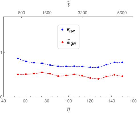
Our numerical simulation results are shown below. For convenience, we denote the number of bubbles of the field $s$ (or field $h$ ) as $N_{\rm b}$ . We simulated three cases in the simulation box with grid points number of $1024^{3}$ , namely pure domain walls (without bubble generation, $N_{\rm b}=0$ ), and the case where 512 or 64 bubbles ( $N_{\rm b}=512$ or $N_{\rm b}=64$ ) are generated during first-order phase transitions. At first, for the simulation of pure domain walls (without bubble generation and ignoring the field $h$ all the time), we measured the scaling parameters ( $\xi_{\rm dw}$ ) of the domain wall network at different times (see the left panel of Fig. S2) and found that the domain wall network entered the scaling regime after $\tilde{\eta}=50$ , and the scaling parameters remained stable at about 1.09. We measured the power spectrum of gravitational waves radiated by pure domain walls (see the middle panel of Fig. S2). The vertical black dashed line in the figure represents the dimensionless comoving wavenumber (momentum) which corresponds to the thickness of the domain wall at the final time

k_{\rm dw,f}=(2\pi/\delta_{\rm dw,f})\times a(\tilde{\eta}_{f})/(a_{i}H_{i}),

(S41)

where $\delta_{\rm dw,f}$ is the physical thickness of the domain wall at the final time $\tilde{\eta}_{f}$ . The physical thickness of the domain wall can be expressed as $\delta_{\rm dw}=1/m_{\rm s,eff}$ , with $m_{\rm s,eff}^{2}=\partial^{2}V(s,0,T)/\partial s^{2}$ the square of the effective mass of the field $s$ . We also measured the efficiency parameter $\epsilon_{\rm gw}$ and differential amplitude $\tilde{\epsilon}_{\rm gw}$ of GWs radiated by the domain-wall network after entering the scaling regime (see the right panel of Fig. S2), they can be expressed as Hiramatsu et al. 2014

\epsilon_{\rm gw}\equiv\frac{\rho_{\rm gw}}{G\xi_{\rm dw}^{2}\sigma_{\rm wall}^{2}},\quad\tilde{\epsilon}_{\rm gw}\equiv\left(\frac{{\rm d}\epsilon_{\rm gw}}{{\rm dln}k}\right)_{\rm peak}=\frac{1}{G\xi_{\rm dw}^{2}\sigma_{\rm wall}^{2}}\left(\frac{{\rm d}\rho_{\rm gw}(t)}{{\rm dln}k}\right)_{\rm peak},

(S42)

where the subscript “peak” implies that the value is computed at the peak of the power spectrum of GWs. We obtain that the average values of $\epsilon_{\rm gw}$ and $\tilde{\epsilon}_{\rm gw}$ are 0.73 and 0.49, respectively.

For intuitiveness, we recorded the three-dimensional distribution of the pure domain wall networks at different times (see Fig. S3).

For the case where 64 bubbles ( $N_{\rm b}=64$ ) are generated during the first order phase transition, the average amplitude of the fields $s$ and $h$ changes as shown in the left panel of Fig. S4. We also measured the power spectrum of gravitational waves in the right plot.

To investigate the impact of the number of grid points ( $N$ ) on our simulation, we performed another set of simulations with $N=512$ points per side. Similarly, We fix $\tilde{\eta}=1$ to be the time at which $T=8T_{\rm c}$ , so the second-order phase transition happens at $\tilde{\eta}=8$ . We still set $f_{*}=\eta=6\times 10^{16}{\rm GeV}$ and $w_{*}=a_{i}H_{i}$ to do the rescale for dimensional physical quantities. We use the second-order leap-frog algorithm to evolve the equations of motion in a simulation box of comoving side-length $L=95/(a_{i}H_{i})$ . So, the dimensionless comoving lattice spacing is about $\delta\tilde{x}=0.19$ (which is equal to the $\delta\tilde{x}$ in the case of $N=1024$ ), and the dimensionless time-step is chosen as $\delta\tilde{\eta}=0.005$ . As the temperature decreases to about $T=0.5v$ , that is, when $\tilde{\eta}=34.68$ , the first-order phase transition happens, and bubbles form in the $s$ and $h$ fields due to quantum tunneling. We evolve the equations of motion until the final moment $\tilde{\eta}=95$ , at this time, the simulation box contains one Hubble volume, and the thickness of the domain walls is about 1.37 times that of the physical lattice spacing.

The evolution of the amplitudes of $s$ and $h$ during the simulation is shown in Fig. S5. We also measured the GW energy density power spectrum at five different moments during the simulation process, see the right panel in the Figure. The evolution of scaling parameters for domain walls is shown in Fig. S6.