Automatic Gradient Descent:
Deep Learning without Hyperparameters

Jeremy Bernstein MIT Chris Mingard U. Oxford Kevin Huang U. Washington Navid Azizan MIT Yisong Yue Caltech

Abstract

The architecture of a deep neural network is defined explicitly in terms of the number of layers, the width of each layer and the general network topology. Existing optimisation frameworks neglect this information in favour of implicit architectural information (e.g. second-order methods) or architecture-agnostic distance functions (e.g. mirror descent). Meanwhile, the most popular optimiser in practice—Adam—is based on heuristics. This paper builds a new framework for deriving optimisation algorithms that explicitly leverage neural architecture. The theory extends mirror descent to non-convex composite objective functions: the idea is to transform a Bregman divergence to account for the non-linear structure of neural architecture. Working through the details for deep fully-connected networks yields automatic gradient descent: a first-order optimiser without any hyperparameters. Automatic gradient descent trains both fully-connected and convolutional networks out-of-the-box and at ImageNet scale. A PyTorch implementation is available at https://github.com/jxbz/agd and also in Appendix B. Overall, the paper supplies a rigorous theoretical foundation for a next-generation of architecture-dependent optimisers that work automatically and without hyperparameters.

$\star$ denotes equal contribution.

Keywords: majorise-minimise meta-algorithm, operator perturbation theory, architecture-aware optimisation

Refer to caption — Figure 1: Automatic gradient descent trains neural networks reliably without hyperparameters. Solid lines show train accuracy and dotted lines show test accuracy. The networks are unregularised with biases and affine parameters disabled, as these features are not yet supported by AGD. In the left panel—unlike AGD—Adam and SGD failed to train a 32-layer fully-connected network on CIFAR-10 with their default learning rates of 0.001 for Adam and 0.1 for SGD. The middle panel displays a learning rate grid search for ResNet-18 trained on CIFAR-10. AGD attained performance comparable to the best tuned performance of Adam and SGD. In the right panel, AGD trained ResNet-50 on ImageNet to a top-1 test accuracy of 65.5%. The ImageNet baseline is SGD with a learning rate of 0.1 and no learning rate decay schedule.

1 Introduction

Automatic differentiation has contributed to the rapid pace of innovation in the field of deep learning. Software packages such as PyTorch (Paszke et al. 2019) and Theano (Al-Rfou et al. 2016) have advanced a programming paradigm where the user (1) defines a neural network architecture by composing differentiable operators and (2) supplies training data. The package then automatically computes the gradient of the error on the training data via recursive application of the chain rule. At this point, the user must become involved again by (3) selecting one of numerous optimisation algorithms and (4) manually tuning its hyperparameters: in particular, the initial learning rate and the learning rate decay schedule (Goodfellow et al. 2016).

But manually tuning hyperparameters is irksome. An abundance of hyperparameters makes it difficult to rank the performance of different deep learning algorithms (Lucic et al. 2017; Schmidt et al. 2021) and difficult to reproduce results in the literature (Henderson et al. 2018). Hyperparameters confound our efforts to build a scientific understanding of generalisation in deep learning (Jiang et al. 2020; Farhang et al. 2022). And, when training neural networks at the largest scale, in pursuit of stronger forms of artificial intelligence, hyperparameter grid search can rack up millions of dollars in compute costs (Sharir et al. 2020).

Are hyperparameters just a fact of life? The thesis of this paper is that no: they are not. Deep learning involves fitting a known function to known data via minimising a known objective. If we could characterise these components both individually and in how they interact, then—in principle—there should be no leftover degrees of freedom to be tuned (Orabona & Cutkosky 2020). Taking this idea and running with it leads to automatic gradient descent (AGD): a neural network optimiser without any hyperparameters. AGD is complementary to automatic differentiation and could help to automate general machine learning workflows.

Two existing tools are central to our derivation, and it is their novel combination that presents the main theoretical contribution of this paper. First, a classic tool from convex analysis known as the Bregman divergence (Bregman 1967; Dhillon & Tropp 2008) is used to characterise how the neural network interacts with the loss function. And second, a tool called deep relative trust (Bernstein et al. 2020) is used to characterise the highly non-linear interaction between the weights and the network output. With these tools in hand, we can apply the majorise-minimise meta-algorithm (Lange 2016) to derive an optimiser explicitly tailored to deep network objective functions. To summarise, the derivation of AGD follows three main steps:

Step 1:

Functional expansion. We use a Bregman divergence to express the linearisation error of the objective function $\mathcal{L}({\bm{w}})$ in terms of the functional perturbation $\Delta{\bm{f}}$ to the network ${\bm{f}}$ .
Step 2:

Architectural perturbation bounds. We use deep relative trust to relate the size and structure of the weight perturbation $\Delta{\bm{w}}$ to the size of the induced functional perturbation $\Delta{\bm{f}}$ .
Step 3:

Majorise-minimise. We substitute deep relative trust into the Bregman divergence to obtain an explicitly architecture-dependent majorisation. Minimising with respect to $\Delta{\bm{w}}$ yields an optimiser.

Summary of contributions

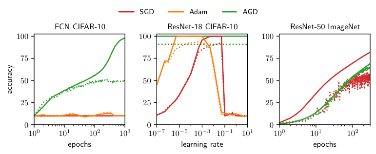
This paper derives automatic gradient descent (AGD) by applying the majorise-minimise meta-algorithm to deep network objective functions. AGD trains all tested network architectures without hyperparameters, and scales to deep networks such as ResNet-50 and large datasets such as ImageNet. AGD trains out-of-the-box even when Adam and SGD fail to train with their default hyperparameters.

Optimiser	Reference	Hyperparameter Free	Width Scaling	Depth Scaling	Automatic Schedule	Memory Cost
Adam	$\mathrlap{\text{\cite[citet]{\@@bibref{Authors Phrase1YearPhrase2}{kingma_adam:_2015}{\@@citephrase{(}}{\@@citephrase{)}}}}}$	✗	✗	✗	✗	$3\times\#$ weights
SGD + mom.	$\mathrlap{\text{\cite[citet]{\@@bibref{Authors Phrase1YearPhrase2}{bottou}{\@@citephrase{(}}{\@@citephrase{)}}}}}$	✗	✗	✗	✗	$2\times\#$ weights
SGD + muP	$\mathrlap{\text{\cite[citet]{\@@bibref{Authors Phrase1YearPhrase2}{Yang2021TensorPI}{\@@citephrase{(}}{\@@citephrase{)}}}}}$	✗	✓	✗	✗	$1\times\#$ weights
AGD	this paper	✓	✓	✓	✓	$1\times\#$ weights

Table 1: Comparing practical optimisers. Adam and momentum-SGD employ running estimates of gradient statistics and thereby use more memory than AGD. In addition, Adam and SGD do not provide guidance on scaling hyperparameters with network architecture, although muP fixes this for the case of width scaling.

1.1 Related work

Optimisation theory

First-order optimisers leverage the first-order Taylor expansion of the objective function $\mathcal{L}({\bm{w}})$ —in particular, the gradient $\nabla_{\bm{w}}\mathcal{L}({\bm{w}})$ . Theoretical treatments include mirror descent (Nemirovsky & Yudin 1983), natural gradient descent (Amari 1998) and the Gauss-Newton method (Björck 1996). These methods have been explored in the context of deep learning (Pascanu & Bengio 2014; Azizan & Hassibi 2019; Sun et al. 2022). First-order methods are amenable to deep learning since the gradient of the objective is available via recursive application of the chain rule—a.k.a. error back-propagation (Rumelhart et al. 1986).

Second-order optimisers leverage the second-order Taylor expansion of the objective function $\mathcal{L}({\bm{w}})$ —in particular, the gradient $\nabla_{\bm{w}}\mathcal{L}({\bm{w}})$ and Hessian $\nabla^{2}_{\bm{w}}\mathcal{L}({\bm{w}})$ . Examples include Newton’s method (Nocedal & Wright 1999) and cubic-regularised Newton’s method (Nesterov & Polyak 2006). Naïvely, second-order methods are less amenable to deep learning since the cost of the relevant Hessian computations is prohibitive at high dimension. That being said, efforts have been made to circumvent this issue (Agarwal et al. 2017).

The majorise-minimise meta-algorithm (Lange 2016) is an algorithmic pattern that can be used to derive optimisers. To apply the meta-algorithm, one must first derive an upper bound on the objective which matches the objective up to $k$ th-order in its Taylor series for some integer $k$ . This majorisation can then be minimised as a proxy for reducing the original objective. Figure 2 illustrates the meta-algorithm for $k=1$ .

Deep learning theory

The Lipschitz smoothness assumption—a global constraint on the eigenvalues of the Hessian—is often used to derive and analyse neural network optimisers (Agarwal et al. 2016). But this assumption has been questioned (Zhang et al. 2020) and evidence has even been found for the reverse relationship, where the Hessian spectrum is highly sensitive to the choice of optimiser (Cohen et al. 2021).

These considerations motivate the development of theory that is more explicitly tailored to neural architecture. For instance, Bernstein et al. 2020 used an architectural perturbation bound termed deep relative trust to characterise the neural network optimisation landscape as a function of network depth. Similarly, Yang & Hu 2021 sought to understand the role of width, leading to their maximal update parameterisation. Tables 1 and 2 provide some points of comparison between automatic gradient descent and these and other frameworks.

Figure 2: Majorise-minimise and the perturbation hierarchy. The left panel depicts the majorise-minimise meta-algorithm (Lange 2016), which is an algorithmic pattern for reducing an objective (blue) by minimising a sequence of upper bounds (one shown in red). The upper bounds, known as a majorisation, must lie tangent to the objective to guarantee an improvement in one step of the meta-algorithm. The right panel depicts the perturbation hierarchy of a generic machine learning model: the optimiser perturbs the weights and this induces perturbations to the model output, the loss on individual training examples and ultimately the overall objective. Majorising machine learning objective functions requires addressing the full perturbation hierarchy.

1.2 Preliminaries

Given a vector ${\bm{v}}$ in $\mathbb{R}^{n}$ , we will need to measure its size in three different ways:

Definition 1 (Manhattan norm).

The Manhattan norm $\|{\,\cdot\,}\|_{1}$ of a vector ${\bm{v}}$ is defined by $\|{{\bm{v}}}\|_{1}\vcentcolon=\sum_{i}|{{\bm{v}}_{i}}|$ .

Definition 2 (Euclidean norm).

The Euclidean norm $\|{\,\cdot\,}\|_{2}$ of a vector ${\bm{v}}$ is defined by $\smash{\|{{\bm{v}}}\|_{2}\vcentcolon=\sqrt{\sum_{i}{\bm{v}}_{i}^{2}}}$ .

Definition 3 (Infinity norm).

The infinity norm $\|{\,\cdot\,}\|_{\infty}$ of a vector ${\bm{v}}$ is defined by $\|{{\bm{v}}}\|_{\infty}\vcentcolon=\max_{i}|{{\bm{v}}_{i}}|$ .

For a matrix ${\bm{M}}$ in $\mathbb{R}^{m\times n}$ , the reader should be aware that it has a singular value decomposition:

Fact 1 (SVD).

Every matrix ${\bm{M}}$ in $\mathbb{R}^{m\times n}$ admits a singular value decomposition (SVD) of the form ${\bm{M}}=\sum_{i=1}^{\min(m,n)}\sigma_{i}({\bm{M}})\cdot{\bm{u}}_{i}{\bm{v}}_{i}^{\top}$ where the left singular vectors $\{{\bm{u}}_{i}\}$ are orthonormal vectors in $\mathbb{R}^{m}$ , the right singular vectors $\{{\bm{v}}_{i}\}$ are orthonormal vectors in $\mathbb{R}^{m}$ and the singular values $\{\sigma_{i}({\bm{M}})\}$ are non-negative scalars.

The singular value decomposition allows us to measure the size of a matrix in two different ways:

Definition 4 (Frobenius norm).

The Frobenius norm $\|{\,\cdot\,}\|_{F}$ of a matrix ${\bm{M}}$ is given by $\|{{\bm{M}}}\|_{F}\vcentcolon=\sqrt{\sum_{i}\sigma_{i}({\bm{M}})^{2}}$ .

Definition 5 (Operator norm).

The operator norm $\|{\,\cdot\,}\|_{*}$ of a matrix ${\bm{M}}$ is given by $\|{{\bm{M}}}\|_{*}\vcentcolon=\max_{i}\sigma_{i}({\bm{M}})$ .

While the operator norm $\|{{\bm{M}}}\|_{*}$ reports the largest singular value, the quantity $\|{{\bm{M}}}\|_{F}/\sqrt{\min(m,n)}$ reports the root mean square singular value. Finally, we will need to understand two aspects of matrix conditioning:

Definition 6 (Rank).

The rank of a matrix counts the number of non-zero singular values.

Definition 7 (Stable rank).

The stable rank of a matrix ${\bm{M}}$ is defined by $\operatorname{rank_{stable}}{\bm{M}}\vcentcolon=\|{{\bm{M}}}\|_{F}^{2}/\|{{\bm{M}}}\|_{*}^{2}$ .

The stable rank provides an approximation to the rank that ignores the presence of very small singular values. Let us consider the extremes. An orthogonal matrix ${\bm{O}}\in\mathbb{R}^{m\times n}$ has both full rank and full stable rank: $\operatorname{rank}{\bm{O}}=\operatorname{rank_{stable}}{\bm{O}}=\min(m,n)$ . A rank-one matrix ${\bm{P}}$ has unit stable rank and satisfies $\|{{\bm{P}}}\|_{*}=\|{{\bm{P}}}\|_{F}$ .

2 Majorise-Minimise for Generic Learning Problems

Theory	Reference	Handles the Loss	Non-Linear Network
mirror descent	$\mathrlap{\text{\cite[citet]{\@@bibref{Authors Phrase1YearPhrase2}{nemirovsky_yudin_1983}{\@@citephrase{(}}{\@@citephrase{)}}}}}$	✓	✗
Gauss-Newton method	Björck 1996	✓	✗
natural gradient descent	Amari 1998	✓	✗
neural tangent kernel	Jacot et al. 2018	✓	✗
deep relative trust	Bernstein et al. 2020	✗	✓
tensor programs	Yang & Hu 2021	✗	✓
automatic gradient descent	this paper	✓	✓

Table 2: Comparing popular frameworks for first-order optimisation theory. Frameworks differ in whether they can handle the interaction between the model output

{\bm{f}}

and the objective

\mathcal{L}

, and the complex non-linear interaction between the weights

{\bm{w}}

and the model output

{\bm{f}}

. Our framework handles both aspects.

This section develops a framework for applying the majorise-minimise meta-algorithm to generic optimisation problems in machine learning. In particular, the novel technique of functional expansion is introduced. Section 3 will apply this technique to deep neural networks. All proofs are supplied in Appendix A.

Given a machine learning model and a set of training data, our objective is to minimise the error of the model, averaged over the training data. Formally, we would like to minimise the following function:

Definition 8 (Composite objective).

Consider a machine learning model ${\bm{f}}$ that maps an input ${\bm{x}}$ and a weight vector ${\bm{w}}$ to output ${\bm{f}}({\bm{x}};{\bm{w}})$ . Given data $\mathsf{S}$ and a convex loss function $\ell$ , the objective $\mathcal{L}({\bm{w}})$ is defined by:

\mathcal{L}({\bm{w}})\vcentcolon=\frac{1}{|\mathsf{S}|}\sum_{({\bm{x}},{\bm{y}})\in\mathsf{S}}\ell({\bm{f}}({\bm{x}};{\bm{w}}),{\bm{y}}).

We refer to this objective as composite since the loss function $\ell$ is composed with a machine learning model ${\bm{f}}$ . While the loss function itself is convex, the overall composite is often non-convex due to the non-linear machine learning model. Common convex loss functions include the square loss and the cross-entropy loss:

Example 1 (Square loss).

The square loss is defined by: $\ell({\bm{f}}({\bm{x}};{\bm{w}}),{\bm{y}})\vcentcolon=\frac{1}{2d_{L}}\|{{\bm{f}}({\bm{x}};{\bm{w}})-{\bm{y}}}\|_{2}^{2}$ .

Example 2 (Xent loss).

The cross-entropy (xent) loss is defined by: $\ell({\bm{f}}({\bm{x}}),{\bm{y}})\vcentcolon=-\log[\operatorname{softmax}({\bm{f}}({\bm{x}}))]^{\top}{\bm{y}}$ , where the softmax function is defined by $\operatorname{softmax}({\bm{f}}({\bm{x}}))\vcentcolon=\exp{\bm{f}}({\bm{x}})/\|{\exp{\bm{f}}({\bm{x}})}\|_{1}$ .

2.1 Decomposition of linearisation error

First-order optimisers leverage the linearisation of the objective at the current iterate. To design such methods, we must understand the realm of validity of this linearisation. To that end, we derive a very general decomposition of the linearisation error of a machine learning system. The result is stated in terms of a perturbation hierarchy. In particular, perturbing the weight vector of a machine learning model ${\bm{w}}\to{\bm{w}}+\Delta{\bm{w}}$ induces perturbations to the model output ${\bm{f}}\to{\bm{f}}+\Delta{\bm{f}}$ , to the loss on individual data samples $\ell\to\ell+\Delta\ell$ and, at last, to the overall objective function $\mathcal{L}\to\mathcal{L}+\Delta\mathcal{L}$ . Formally, a weight perturbation $\Delta{\bm{w}}$ induces:

$\displaystyle\Delta{\bm{f}}({\bm{x}})$	$\displaystyle\coloneqq{\bm{f}}({\bm{x}};{\bm{w}}+\Delta{\bm{w}})-{\bm{f}}({\bm{x}};{\bm{w}});\hskip 160.00024pt$	(functional perturbation)
$\displaystyle\Delta\ell({\bm{f}}({\bm{x}}),{\bm{y}})$	$\displaystyle\coloneqq\ell({\bm{f}}({\bm{x}})+\Delta{\bm{f}}({\bm{x}}),{\bm{y}})-\ell({\bm{f}}({\bm{x}}),{\bm{y}});$	(loss perturbation)
$\displaystyle\Delta\mathcal{L}({\bm{w}})$	$\displaystyle\coloneqq\textstyle\frac{1}{\|\mathsf{S}\|}\sum_{({\bm{x}},{\bm{y}})\in\mathsf{S}}\Delta\ell({\bm{f}}({\bm{x}}),{\bm{y}}).$	(objective perturbation)

We have adopted a compact notation where the dependence of ${\bm{f}}({\bm{x}};{\bm{w}})$ on ${\bm{w}}$ is at times suppressed. The perturbation hierarchies of a generic machine learning model and a deep neural network are visualised in Figures 2 and 3, respectively. The linearisation error of the objective perturbation $\Delta\mathcal{L}$ decomposes as:

Proposition 1 (Decomposition of linearisation error).

For any differentiable loss $\ell$ and any differentiable machine learning model ${\bm{f}}$ the linearisation error of the objective function $\mathcal{L}$ admits the following decomposition:

	$\displaystyle\quad\quad\quad\underbrace{\Delta\mathcal{L}({\bm{w}})-\nabla_{\bm{w}}\mathcal{L}({\bm{w}})^{\top}\Delta{\bm{w}}}_{\mathclap{\text{linearisation error of objective}}}\quad\quad$	$\displaystyle=$		$\displaystyle\frac{1}{\|\mathsf{S}\|}\sum_{({\bm{x}},{\bm{y}})\in\mathsf{S}}\nabla_{{\bm{f}}({\bm{x}})}\ell({\bm{f}}({\bm{x}}),{\bm{y}})^{\top}\underbrace{\left[\Delta{\bm{f}}({\bm{x}})-\nabla_{\bm{w}}{\bm{f}}({\bm{x}})\Delta{\bm{w}}\right]}_{\mathclap{\text{linearisation error of model}}}$
	$\displaystyle+\,$	$\displaystyle\frac{1}{\|\mathsf{S}\|}\sum_{({\bm{x}},{\bm{y}})\in\mathsf{S}}\underbrace{\Delta\ell({\bm{f}}({\bm{x}}),{\bm{y}})-\nabla_{{\bm{f}}({\bm{x}})}\ell({\bm{f}}({\bm{x}}),{\bm{y}})^{\top}\Delta{\bm{f}}({\bm{x}})}_{\text{linearisation error of loss}}.\quad\quad\quad$

In words: the linearisation error of the objective decomposes into two terms. The first depends on the linearisation error of the machine learning model and the second the loss. This decomposition relies on nothing but differentiability. For a convex loss, the second term may be interpreted as a Bregman divergence:

Definition 9 (Bregman divergence of loss).

For any convex loss $\ell$ :

\displaystyle\qquad\qquad\qquad\qquad\operatorname{bregman}_{\ell(\cdot,{\bm{y}})}({\bm{f}}({\bm{x}}),\Delta{\bm{f}}({\bm{x}}))\vcentcolon=\Delta\ell({\bm{f}}({\bm{x}}),{\bm{y}})-\nabla_{{\bm{f}}({\bm{x}})}\ell({\bm{f}}({\bm{x}}),{\bm{y}})^{\top}\Delta{\bm{f}}({\bm{x}}).

A Bregman divergence is just the linearisation error of a convex function. Two important examples are:

Figure 3: Perturbation hierarchy of a deep neural network. When training a neural network, the optimiser applies structured perturbations to the weights, in the form of one perturbation matrix

\Delta{\bm{W}}_{k}

per weight matrix

{\bm{W}}_{k}

. Deep relative trust (Bernstein et al. 2020) provides a tool to understand how structured weight perturbations of this form affect the network output

{\bm{f}}

. Combining deep relative trust with a Bregman divergence (Bregman 1967) allows us to analyse the full perturbation hierarchy.

Lemma 1 (Bregman divergence of square loss).

When $\ell$ is set to square loss, then:

\displaystyle\qquad\qquad\qquad\qquad\operatorname{bregman}_{\ell(\cdot,{\bm{y}})}({\bm{f}}({\bm{x}}),\Delta{\bm{f}}({\bm{x}}))=\tfrac{1}{2d_{L}}\|{\Delta{\bm{f}}({\bm{x}})}\|_{2}^{2}.

Lemma 2 (Bregman divergence of xent loss).

When $\ell$ is set to cross-entropy loss, and if ${\bm{y}}^{\top}\bm{1}=1$ , then:

	$\displaystyle\qquad\qquad\qquad\qquad\operatorname{bregman}_{\ell(\cdot,{\bm{y}})}({\bm{f}}({\bm{x}}),\Delta{\bm{f}}({\bm{x}}))$	$\displaystyle=D_{\mathrm{KL}}\Big(\operatorname{softmax}({\bm{f}}({\bm{x}}))\,\Big\|\Big\|\,\operatorname{softmax}({\bm{f}}({\bm{x}})+\Delta{\bm{f}}({\bm{x}}))\Big)$
		$\displaystyle\leq\tfrac{1}{2}\\|{\Delta{\bm{f}}({\bm{x}})}\\|_{\infty}^{2}+\mathcal{O}(\Delta{\bm{f}}^{3}).$

Our methods may be applied to other convex losses by calculating or bounding their Bregman divergence.

2.2 Functional expansion and functional majorisation

Before continuing, we make one simplifying assumption. Observe that the first term on the right-hand side of Proposition 1 is a high-dimensional inner product between two vectors. Since there is no clear reason why these two vectors should be aligned, let us assume that their inner product is zero:

Assumption 1 (Orthogonality of model linearisation error).

In the same setting as Proposition 1:

\frac{1}{|\mathsf{S}|}\sum_{({\bm{x}},{\bm{y}})\in\mathsf{S}}\nabla_{{\bm{f}}({\bm{x}})}\ell({\bm{f}}({\bm{x}}),{\bm{y}})^{\top}\underbrace{\left[\Delta{\bm{f}}({\bm{x}})-\nabla_{\bm{w}}{\bm{f}}({\bm{x}})\Delta{\bm{w}}\right]}_{\mathclap{\text{linearisation error of model}}}=0.

While it is possible to work without this assumption (Bernstein 2022), we found that its inclusion simplifies the analysis and in practice did not lead to a discernible weakening of the resulting algorithm. In any case, this assumption is considerably milder than the common assumption in the literature (Pascanu & Bengio 2014; Lee et al. 2019) that the model linearisation error is itself zero: $\left[\Delta{\bm{f}}({\bm{x}})-\nabla_{\bm{w}}{\bm{f}}({\bm{x}})\Delta{\bm{w}}\right]=0$ .

Armed with Proposition 1 and 1, we are ready to introduce functional expansion and majorisation:

Theorem 1 (Functional expansion).

Consider a convex differentiable loss $\ell$ and a differentiable machine learning model ${\bm{f}}$ . Under 1, the corresponding composite objective $\mathcal{L}$ admits the expansion:

\displaystyle\mathcal{L}({\bm{w}}+\Delta{\bm{w}})=\underbrace{\mathcal{L}({\bm{w}})+\nabla_{\bm{w}}\mathcal{L}({\bm{w}})^{\top}\Delta{\bm{w}}}_{\text{first-order Taylor series}}+\frac{1}{|\mathsf{S}|}\sum_{({\bm{x}},{\bm{y}})\in\mathsf{S}}\operatorname{bregman}_{\ell(\cdot,{\bm{y}})}({\bm{f}}({\bm{x}}),\Delta{\bm{f}}({\bm{x}})).

So the perturbed objective $\mathcal{L}({\bm{w}}+\Delta{\bm{w}})$ may be written as the sum of its first-order Taylor expansion with a Bregman divergence in the model outputs averaged over the training set. It is straightforward to specialise this result to different losses by substituting in their Bregman divergence:

Corollary 1 (Functional expansion of mean squared error).

Under 1, for square loss:

\displaystyle\qquad\qquad\qquad\qquad\mathcal{L}({\bm{w}}+\Delta{\bm{w}})=\mathcal{L}({\bm{w}})+\nabla_{\bm{w}}\mathcal{L}({\bm{w}})^{\top}\Delta{\bm{w}}+\frac{1}{|\mathsf{S}|}\sum_{({\bm{x}},{\bm{y}})\in\mathsf{S}}\tfrac{1}{2d_{L}}\|{\Delta{\bm{f}}({\bm{x}})}\|_{2}^{2}.

Corollary 2 (Functional majorisation for xent loss).

Under 1, for cross-entropy loss, if ${\bm{y}}^{\top}\bm{1}=1$ :

\displaystyle\qquad\qquad\qquad\qquad\mathcal{L}({\bm{w}}+\Delta{\bm{w}})\leq\mathcal{L}({\bm{w}})+\nabla_{\bm{w}}\mathcal{L}({\bm{w}})^{\top}\Delta{\bm{w}}+\frac{1}{|\mathsf{S}|}\sum_{({\bm{x}},{\bm{y}})\in\mathsf{S}}\tfrac{1}{2}\|{\Delta{\bm{f}}({\bm{x}})}\|_{\infty}^{2}+\mathcal{O}(\Delta{\bm{f}}^{3}).

When the functional perturbation is reasonably “spread out”, we would expect $\|{\Delta{\bm{f}}({\bm{x}})}\|_{\infty}^{2}\approx\|{\Delta{\bm{f}}({\bm{x}})}\|_{2}^{2}/d_{L}$ . In this setting, the functional majorisation of cross-entropy loss agrees with the functional expansion of mean squared error to second order. While the paper derives automatic gradient descent for the square loss, this observation justifies its application to cross-entropy loss, as in the case of the ImageNet experiments.

2.3 Recovering existing frameworks

We briefly observe that three existing optimisation frameworks may be recovered efficiently from Theorem 1:

Mirror descent

For linear models ${\bm{f}}({\bm{x}};{\bm{W}})\vcentcolon={\bm{W}}{\bm{x}}$ , the Bregman divergence $\operatorname{bregman}_{\ell(\cdot,{\bm{y}})}({\bm{f}}({\bm{x}}),\Delta{\bm{f}}({\bm{x}}))$ may be written $\operatorname{bregman}_{\ell(\cdot,{\bm{y}})}({\bm{W}}{\bm{x}},\Delta{\bm{W}}{\bm{x}})$ . This is a convex function of the weight perturbation $\Delta{\bm{W}}$ . Substituting into Theorem 1 and minimising with respect to $\Delta{\bm{W}}$ is the starting point for mirror descent.

Gauss-Newton method

Substituting the linearised functional perturbation $\Delta{\bm{f}}({\bm{x}})\approx\nabla_{\bm{w}}{\bm{f}}({\bm{x}})\Delta{\bm{w}}$ into Corollary 1 and minimising with respect to $\Delta{\bm{w}}$ is the starting point for the Gauss-Newton method.

Natural gradient descent

Substituting the linearised functional perturbation $\Delta{\bm{f}}({\bm{x}})\approx\nabla_{\bm{w}}{\bm{f}}({\bm{x}})\Delta{\bm{w}}$ into Corollary 2 and minimising with respect to $\Delta{\bm{w}}$ is the starting point for natural gradient descent.

3 Majorise-Minimise for Deep Learning Problems

In this section, we will focus our efforts on deriving an optimiser for deep fully-connected networks trained with square loss. The derivation for cross-entropy loss is analogous. Proofs are relegated to Appendix A.

Definition 10 (Fully-connected network).

A fully-connected network (FCN) ${\bm{f}}$ of depth $L$ maps an input ${\bm{x}}\in\mathbb{R}^{d_{0}}$ to an output ${\bm{f}}({\bm{x}};{\bm{w}})\in\mathbb{R}^{d_{L}}$ via $L$ matrix multiplications interspersed by non-linearity $\operatorname{relu}(z)\vcentcolon=\max(0,z)$ :

{\bm{f}}({\bm{x}};{\bm{w}})\coloneqq{\bm{W}}_{L}\circ(\operatorname{relu}{}\circ{\bm{W}}_{L-1})\circ(\operatorname{relu}{}\circ{\bm{W}}_{L-2})\circ\dots\circ(\operatorname{relu}{}\circ{\bm{W}}_{1}{\bm{x}}).

In this expression, ${\bm{w}}$ denotes the tuple of matrices ${\bm{w}}=({\bm{W}}_{1},...,{\bm{W}}_{L})$ with $k$ th matrix ${\bm{W}}_{k}$ in $\mathbb{R}^{d_{k}\times d_{k-1}}$ . In what follows, we will find the following dimensional scaling to be particularly convenient:

Prescription 1 (Dimensional scaling).

For $\eta>0$ , the data $({\bm{x}},{\bm{y}})$ , weights ${\bm{W}}_{k}$ and updates $\Delta{\bm{W}}_{k}$ should obey:

$\displaystyle\\|{{\bm{x}}}\\|_{2}$	$\displaystyle=\sqrt{d_{0}};$	(input scaling)
$\displaystyle\\|{{\bm{W}}_{k}}\\|_{*}$	$\displaystyle=\sqrt{d_{k}/d_{k-1}}\hskip 15.18999pt\qquad\text{for all }k=1,...,L;$	(weight scaling)
$\displaystyle\\|{\Delta{\bm{W}}_{k}}\\|_{*}$	$\displaystyle=\sqrt{d_{k}/d_{k-1}}\cdot\tfrac{\eta}{L}\qquad\text{for all }k=1,...,L;$	(update scaling)
$\displaystyle\\|{{\bm{y}}}\\|_{2}$	$\displaystyle=\sqrt{d_{L}}.$	(target scaling)

While results can be derived without adopting 1, the scalings substantially simplify our formulae. One reason for this is that, under 1, we have the telescoping property that $\prod_{k=1}^{L}\|{{\bm{W}}_{k}}\|_{*}=\sqrt{d_{L}/d_{0}}$ . For a concrete example of how this helps, consider the following bound on the norm of the network outputs:

Lemma 3 (Output bound).

The output norm of a fully-connected network ${\bm{f}}$ obeys the following bound:

\displaystyle\|{{\bm{f}}({\bm{x}};{\bm{w}})}\|_{2}

\displaystyle\leq\left[\prod_{k=1}^{L}\|{{\bm{W}}_{k}}\|_{*}\right]\times\|{{\bm{x}}}\|_{2}=\sqrt{d_{L}}\text{ under \lx@cref{creftype\lx@tilde refnum}{prescription:norm}}.

So, under 1, the bound is simple. Furthermore, the scaling of the update with a single parameter $\eta$ reduces the problem of solving for an optimiser to a single parameter problem. To see how this might make life easier, consider the following lemma that relates weight perturbations to functional perturbations:

Lemma 4 (Deep relative trust).

When adjusting the weights ${\bm{w}}=({\bm{W}}_{1},...,{\bm{W}}_{L})$ of a fully-connected network ${\bm{f}}$ by $\Delta{\bm{w}}=(\Delta{\bm{W}}_{1},...,\Delta{\bm{W}}_{L})$ , the induced functional perturbation $\Delta{\bm{f}}({\bm{x}})\vcentcolon={\bm{f}}({\bm{x}};{\bm{w}}+\Delta{\bm{w}})-{\bm{f}}({\bm{x}};{\bm{w}})$ obeys:

\displaystyle\|{\Delta{\bm{f}}({\bm{x}})}\|_{2}

\displaystyle\leq\left[\prod_{k=1}^{L}\|{{\bm{W}}_{k}}\|_{*}\right]\times\|{{\bm{x}}}\|_{2}\times\left[\prod_{k=1}^{L}\left(1+\frac{\|\Delta{\bm{W}}_{k}\|_{*}}{\|{\bm{W}}_{k}\|_{*}}\right)-1\right]\leq\sqrt{d_{L}}\times(\exp\eta-1)\text{ under \lx@cref{creftype\lx@tilde refnum}{prescription:norm}}.

So, under 1, the single parameter $\eta$ directly controls the size of functional perturbations.

In terms of enforcing 1 in practice, the norms of the data $({\bm{x}},{\bm{y}})$ may be set via pre-processing, the norm of the update $\Delta{\bm{W}}_{k}$ may be set via the optimisation algorithm and the norm of the weight matrix ${\bm{W}}_{k}$ may be set by the choice of initialisation. While, yes, $\|{{\bm{W}}_{k}}\|_{*}$ may drift during training, the amount that this can happen is limited by Weyl 1912’s inequality for singular values. In particular, after one step the perturbed operator norm $\|{{\bm{W}}_{k}+\Delta{\bm{W}}_{K}}\|_{*}$ is sandwiched like $(1-\eta/L)\cdot\|{{\bm{W}}_{k}}\|_{*}\leq\|{{\bm{W}}_{k}+\Delta{\bm{W}}_{K}}\|_{*}\leq(1+\eta/L)\cdot\|{{\bm{W}}_{k}}\|_{*}$ .

def initialise_weights():

for layer

k

\{1,...,L\}

{\bm{W}}_{k}\sim\textsc{uniform}(\mathtt{orthogonal}(d_{k},d_{k-1}))

\#

sample a semi-orthogonal matrix

{\bm{W}}_{k}\leftarrow{\bm{W}}_{k}\cdot\sqrt{\frac{d_{k}}{d_{k-1}}}

\#

rescale its singular values

def update_weights():

G\leftarrow\frac{1}{L}\sum_{l=1}^{L}\|{\nabla_{{\bm{W}}_{k}}\mathcal{L}}\|_{F}\cdot\sqrt{\frac{d_{k}}{d_{k-1}}}

\#

get gradient summary

\smash{\eta\leftarrow\log\frac{1+\sqrt{1+4G}}{2}}

\#

set automatic learning rate

for layer

k

\{1,...,L\}

{\bm{W}}_{k}\leftarrow{\bm{W}}_{k}-\frac{\eta}{L}\cdot\frac{\nabla_{{\bm{W}}_{k}}\mathcal{L}}{\|{\nabla_{{\bm{W}}_{k}}\mathcal{L}}\|_{F}}\cdot\sqrt{\frac{d_{k}}{d_{k-1}}}

\#

update weights

Algorithm 1 Automatic gradient descent. The matrix

{\bm{W}}_{k}

\mathbb{R}^{d_{k}\times d_{k-1}}

is the weight matrix at layer

k

. The gradient

\nabla_{{\bm{W}}_{k}}\mathcal{L}

is with respect to the objective

\mathcal{L}

evaluated on a mini-batch

B

of training samples.

3.1 Deriving automatic gradient descent

With both functional majorisation and deep relative trust in hand, we can majorise the deep network objective:

Lemma 5 (Exponential majorisation).

For an FCN with square loss, under 1 and 1:

\mathcal{L}({\bm{w}}+\Delta{\bm{w}})\leq\mathcal{L}({\bm{w}})+\frac{\eta}{L}\sum_{k=1}^{L}\left[\sqrt{d_{k}/d_{k-1}}\times\operatorname{tr}\frac{\Delta{\bm{W}}_{k}^{\top}\nabla_{{\bm{W}}_{k}}\mathcal{L}}{\|{\Delta{\bm{W}}_{k}}\|_{*}}\right]+\tfrac{1}{2}\,(\exp\eta-1)^{2}.

Observe that the majorisation only depends on the magnitude of the scalar $\eta$ and on some notion of angle $\operatorname{tr}\Delta{\bm{W}}_{k}^{\top}\nabla_{{\bm{W}}_{k}}\mathcal{L}/\|{\Delta{\bm{W}}_{k}}\|_{*}$ between the perturbation matrix $\Delta{\bm{W}}_{k}$ and the gradient matrix $\nabla_{{\bm{W}}_{k}}\mathcal{L}$ . To derive an optimiser, we would now like to minimise this majorisation with respect to $\eta$ and this angle. First, let us introduce one additional assumption and one additional definition:

Assumption 2 (Gradient conditioning).

The gradient satisfies $\operatorname{rank_{stable}}\nabla_{{\bm{W}}_{k}}\mathcal{L}=1$ at all layers $k=1,...,L$ .

This assumption implies that the Frobenius norm $\|{\nabla_{{\bm{W}}_{k}}\mathcal{L}}\|_{F}$ and operator norm $\|{\nabla_{{\bm{W}}_{k}}\mathcal{L}}\|_{*}$ of the gradient at layer $k$ are equal. It is not immediately obvious why this should be a good assumption. After all, the gradient is a sum of $|{\mathsf{S}}|$ rank-one matrices: $\nabla_{{\bm{W}}_{k}}\mathcal{L}=\tfrac{1}{|{\mathsf{S}}|}\sum_{({\bm{x}},{\bm{y}})\in\mathsf{S}}\nabla_{{\bm{h}}_{k}}\ell({\bm{f}}({\bm{x}}),{\bm{y}})\otimes{\bm{h}}_{k-1}$ , where ${\bm{h}}_{k-1}({\bm{x}})$ and ${\bm{h}}_{k}({\bm{x}})$ denote the inputs and outputs of the weight matrix ${\bm{W}}_{k}$ at layer $k$ , and $\otimes$ denotes the outer product. So, naïvely, one might expect the gradient $\nabla_{{\bm{W}}_{k}}\mathcal{L}$ to have a stable rank of $\min(d_{k},d_{k-1},|{\mathsf{S}}|)$ . But it turns out to be a good assumption in practice (Yang & Hu 2021; Yang et al. 2021). And for the definition:

Definition 11 (Gradient summary).

At a weight setting ${\bm{w}}$ , the gradient summary $G$ is given by:

\displaystyle G

\displaystyle\vcentcolon=\frac{1}{L}\sum_{k=1}^{L}\sqrt{d_{k}/d_{k-1}}\cdot\|{\nabla_{{\bm{W}}_{k}}\mathcal{L}({\bm{w}})}\|_{F}.

The gradient summary is a weighted average of gradient norms over layers. It can be thought of as a way to measure the size of the gradient while accounting for the fact that the weight matrices at different layers may be on different scales. This is related to the concept of the gradient scale coefficient of Philipp et al. 2017.

We now have everything we need to derive automatic gradient descent via the majorise-minimise principle:

Theorem 2 (Automatic gradient descent).

For a deep fully-connected network, under 1 and 2 and 1, the majorisation of square loss given in Lemma 5 is minimised by setting:

\displaystyle\eta=\log\frac{1+\sqrt{1+4G}}{2},\qquad\Delta{\bm{W}}_{k}=-\frac{\eta}{L}\cdot\sqrt{d_{k}/d_{k-1}}\cdot\frac{\nabla_{{\bm{W}}_{k}}\mathcal{L}}{\|{\nabla_{{\bm{W}}_{k}}\mathcal{L}}\|_{F}},\qquad\text{for all layers }k=1,...,L.

We present pseudocode for this theorem in Algorithm 1, and a PyTorch implementation in Appendix B. Via a simple derivation based on clear algorithmic principles, automatic gradient descent unifies various heuristic and theoretical ideas that have appeared in the literature:

•

Relative updates. The update is scaled relative to the norm of the weight matrix to which it is applied—assuming the weight matrices are scaled according to 1. Such a scaling was proposed by You et al. 2017 and further explored by Carbonnelle & Vleeschouwer 2019 and Bernstein et al. 2020. There is evidence that such relative synaptic updates may occur in neuroscience (Loewenstein et al. 2011).
•

Depth scaling. Scaling the perturbation strength like $1/L$ for networks of depth $L$ was proposed on theoretical grounds by Bernstein et al. 2020 based on analysis via deep relative trust.
•

Width scaling. The dimensional factors of $d_{k}$ and $d_{k-1}$ that appear closely relate to the maximal update parameterisation of Yang & Hu 2021 designed to ensure hyperparameter transfer across network width.
•

Gradient clipping. The logarithmic dependence of the update on the gradient summary may be seen as an automatic form of adaptive gradient clipping (Brock et al. 2021)—a technique which clips the gradient once its magnitude surpasses a certain threshold set by a hyperparameter.

3.2 Convergence analysis

This section presents theoretical convergence rates for automatic gradient descent. While the spirit of the analysis is standard in optimisation theory, the details may still prove interesting for their detailed characterisation of the optimisation properties of deep networks. For instance, we propose a novel Polyak-Łojasiewicz inequality tailored to the operator structure of deep networks. We begin with two observations:

Lemma 6 (Bounded objective).

For square loss, the objective is bounded as follows:

\displaystyle\mathcal{L}({\bm{w}})

\displaystyle\leq\frac{1}{|{\mathsf{S}}|}\sum_{({\bm{x}},{\bm{y}})\in\mathsf{S}}\frac{\|{{\bm{f}}({\bm{x}};{\bm{w}})}\|_{2}^{2}+\|{{\bm{y}}}\|_{2}^{2}}{2d_{L}}\leq 1\text{ under \lx@cref{creftype\lx@tilde refnum}{prescription:norm}.}

Lemma 7 (Bounded gradient).

For square loss, the norm of the gradient at layer $k$ is bounded as follows:

\displaystyle\|{\nabla_{{\bm{W}}_{k}}\mathcal{L}}\|_{F}

\displaystyle\leq\frac{\prod_{l=1}^{L}\|{{\bm{W}}_{l}}\|_{*}}{\|{{\bm{W}}_{k}}\|_{*}}\cdot\sqrt{\frac{2\mathcal{L}({\bm{w}})}{d_{L}}}\cdot\sqrt{\frac{1}{|{\mathsf{S}}|}\sum_{({\bm{x}},{\bm{y}})\in\mathsf{S}}\|{{\bm{x}}}\|_{2}^{2}}\leq\sqrt{2\cdot\frac{d_{k-1}}{d_{k}}}\text{ under \lx@cref{creftype\lx@tilde refnum}{prescription:norm}.}

These results help us prove that automatic gradient descent converges to a point where the gradient vanishes:

Lemma 8 (Convergence rate to critical point).

Consider a fully-connected network trained by automatic gradient descent (Theorem 2) and square loss for $T$ iterations. Let $G_{t}$ denote the gradient summary (Definition 11) at step $t\leq T$ . Under 1 and 2 and 1, AGD converges at the following rate:

\min_{t\in\{1,...,T\}}G_{t}^{2}\leq\frac{11}{T}.

This lemma can be converted into a convergence rate to a global minimum with one additional assumption:

Assumption 3 (Deep Polyak-Łojasiewicz inequality).

For some $\alpha>0$ , the gradient norm is lower bounded by:

\displaystyle\|{\nabla_{{\bm{W}}_{k}}\mathcal{L}}\|_{F}

\displaystyle\geq\alpha\times\frac{\prod_{l=1}^{L}\|{{\bm{W}}_{l}}\|_{*}}{\|{{\bm{W}}_{k}}\|_{*}}\cdot\sqrt{\frac{2\mathcal{L}({\bm{w}})}{d_{L}}}\cdot\sqrt{\frac{1}{|{\mathsf{S}}|}\sum_{({\bm{x}},{\bm{y}})\in\mathsf{S}}\|{{\bm{x}}}\|_{2}^{2}}=\alpha\times\sqrt{2\cdot\mathcal{L}({\bm{w}})\cdot\frac{d_{k-1}}{d_{k}}}\text{ under \lx@cref{creftype\lx@tilde refnum}{prescription:norm}.}

This lower bound mirrors the structure of the upper bound in Lemma 7. The parameter $\alpha$ captures how much of the gradient is attenuated by small singular values in the weights and by deactivated $\operatorname{relu}$ units. While Polyak-Łojasiewicz inequalities are common in the literature (Liu et al. 2022), our assumption is novel in that it pays attention to the operator structure of the network. 3 leads to the following theorem:

Theorem 3 (Convergence rate to global minima).

For automatic gradient descent (Theorem 2) in the same setting as Lemma 8 but with the addition of 3, the mean squared error objective at step $T$ obeys:

\displaystyle\mathcal{L}({\bm{w}}_{T})\leq\frac{1}{\alpha^{2}}\times\frac{6}{T}.

3.3 Experiments

The goal of our experiments was twofold. First, we wanted to test automatic gradient descent (AGD, Algorithm 1) on a broad variety of networks architectures and datasets to check that it actually works. In particular, we tested AGD on fully-connected networks (FCNs, Definition 10), and both VGG-style (Simonyan & Zisserman 2015) and ResNet-style (He et al. 2015) convolutional neural networks on the CIFAR-10, CIFAR-100 (Krizhevsky 2009) and ImageNet (Deng et al. 2009, ILSVRC2012) datasets with standard data augmentation. And second, to see what AGD may have to offer beyond the status quo, we wanted to compare AGD to tuned Adam and SGD baselines, as well as Adam and SGD run with their default hyperparameters.

To get AGD working with convolutional layers, we adopted a per-submatrix normalisation scheme. Specifically, for a convolutional tensor with filters of size $\mathtt{k_{x}}\times\mathtt{k_{y}}$ , we implemented the normalisation separately for each of the $\mathtt{k_{x}}\times\mathtt{k_{y}}$ submatrices of dimension $\mathtt{channels_{in}}\times\mathtt{channels_{out}}$ . Since AGD does not yet support biases or affine parameters in batchnorm, we disabled these parameters in all architectures. To at least adhere to 1 at initialisation, AGD draws initial weight matrices uniform semi-orthogonal and re-scaled by a factor of $\sqrt{\mathtt{fan\_in}/\mathtt{fan\_out}}$ . Adam and SGD baselines used the PyTorch default initialisation. A PyTorch implementation of AGD reflecting these details is given in Appendix B. All experiments use square loss except ImageNet which used cross-entropy loss. Cross-entropy loss has been found to be superior to square loss for datasets with a large number of classes (Demirkaya et al. 2020; Hui & Belkin 2021).

Our experimental results are spread across five figures:

•

Figure 1 presents some highlights of our results: First, AGD can train networks that Adam and SGD with default hyperparameters cannot. Second, for ResNet-18 on CIFAR-10, AGD attained performance comparable to the best-tuned performance of Adam and SGD. And third, AGD scales up to ImageNet.
•

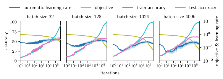
Figure 4 displays the breadth of our experiments: from training a 16-layer fully-connected network on CIFAR-10 to training ResNet-50 on ImageNet. Adam’s learning rate was tuned over the logarithmic grid $\{10^{-5},10^{-4},...,10^{-1}\}$ while for ImageNet we used a default learning rate of 0.1 for SGD without any manual decay. AGD and Adam performed almost equally well on the depth-16 width-512 fully-connected network: 52.7% test accuracy for AGD compared to 53.5% for Adam. For ResNet-18 on CIFAR-10, Adam attained 92.9% test accuracy compared to AGD’s 91.2%. On this benchmark, a fully-tuned SGD with learning rate schedule, weight decay, cross-entropy loss and bias and affine parameters can attain 93.0% test accuracy (Liu 2017). For VGG-16 on CIFAR-100, AGD achieved 67.4% test accuracy compared to Adam’s 69.7%. Finally, on ImageNet AGD achieved a top-1 test accuracy of 65.5% after 350 epochs.
•

Figure 5 compares AGD to Adam and SGD for training an eight-layer fully-connected network of width 256. Adam and SGD’s learning rates were tuned over the logarithmic grid $\{10^{-5},10^{-4},...,10^{-1}\}$ . Adam’s optimal learning rate of $10^{-4}$ was three orders of magnitude smaller than SGD’s optimal learning rate of $10^{-1}$ . SGD did not attain as low of an objective value as Adam or AGD.
•

Figure 6 shows that AGD can train FCNs with width ranging from 64 to 2048 and depth from 2 to 32 and Figure 7 shows that AGD successfully trains a four-layer FCN at varying mini-batch size: from 32 to 4096.

Figure 5: Comparing automatic gradient descent to tuned Adam and SGD. An eight-layer fully-connected network was trained on CIFAR-10 with square loss. Dotted lines show test and solid lines show train performance. The left panel shows the objective value: AGD and Adam attained a smaller training objective than SGD. The middle panel shows train and test accuracies. The right panel shows the relative update size averaged over layers:

\tfrac{1}{L}\sum_{k=1}^{L}\|{\Delta{\bm{W}}_{k}}\|_{F}/\|{{\bm{W}}_{k}}\|_{F}

. We plot the maximum, minimum and mean over an epoch.

4 Discussion

This paper has proposed a new framework for deriving optimisation algorithms for non-convex composite objective functions, which are particularly prevalent in the field of machine learning and the subfield of deep learning. What we have proposed is truly a framework: it can be applied to a new loss function by writing down its Bregman divergence, or a new machine learning model by writing down its architectural perturbation bound. The framework is properly placed in the context of existing frameworks such as the majorise-minimise meta-algorithm, mirror descent and natural gradient descent.

Recent papers have proposed a paradigm of hyperparameter transfer where a small network is tuned and the resulting hyperparameters are transferred to a larger network (Yang et al. 2021; Bernstein 2022). The methods and results in this paper suggest a stronger paradigm of hyperparameter elimination: by detailed analysis of the structure and interactions between different components of a machine learning system, we may hope—if not to outright outlaw hyperparameters—at least to reduce their abundance and opacity.

The main product of this research is automatic gradient descent (AGD), with pseudocode given in Algorithm 1 and PyTorch code given in Appendix B. We have found AGD to be genuinely useful, and believe that it may complement automatic differentiation in helping to automate general machine learning workflows.

The analysis leading to automatic gradient descent is elementary: we leverage basic concepts in linear algebra such as matrix and vector norms, and use simple bounds such as the triangle inequality for vector–vector sums, and the operator norm bound for matrix–vector products. The analysis is non-asymptotic: it does not rely on taking dimensions to infinity, and deterministic: it does not involve random matrix theory. We believe that the accessibility of the analysis could make this paper a good starting point for future developments.

Directions for future work

Here we list some promising avenues for theoretical and practical research. We are exploring some of these ideas in our development codebase: https://github.com/C1510/agd_exp.

•

Stochastic optimisation. Automatic gradient descent is derived in the full-batch optimisation setting, but the algorithm is evaluated experimentally in the mini-batch setting. It would be interesting to try to extend our theoretical and practical methods to more faithfully address stochastic optimisation.
•

More architectures. Automatic gradient descent is derived for fully-connected networks and extended heuristically to convolutional networks. We are curious to extend the methods to more varied architectures such as transformers (Vaswani et al. 2017) and architectural components such as biases. Since most neural networks resemble fully-connected networks in the sense that they are all just deep compound operators, we expect much of the structure of automatic gradient descent as presented to carry through.
•

Regularisation. The present paper deals purely with the optimisation structure of deep neural networks, and little thought is given to either generalisation or regularisation. Future work could look at both theoretical and practical regularisation schemes for automatic gradient descent. It would be interesting to try to do this without introducing hyperparameters, although we suspect that when it comes to regularisation at least one hyperparameter may become necessary.
•

Acceleration. We have found in some preliminary experiments that slightly increasing the update size of automatic gradient descent with a gain hyperparameter, or introducing a momentum hyperparameter, can lead to faster convergence. We emphasise that no experiment in this paper used such hyperparameters. Still, these observations may provide a valuable starting point for improving AGD in future work.
•

Operator perturbation theory. Part of the inspiration for this paper was the idea of applying operator perturbation theory to deep learning. While perturbation theory is well-studied in the context of linear operators (Weyl 1912; Kato 1966; Stewart 2006), in deep learning we are concerned with non-linear compound operators. It may be interesting to try to further extend results in perturbation theory to deep neural networks. One could imagine cataloging the perturbation structure of different neural network building blocks, and using a result similar to deep relative trust (Lemma 4) to describe how they compound.

Acknowledgments

The authors are grateful to MIT SuperCloud, Oxford Hydra, NVIDIA and Virgile Richard for providing GPUs. Thanks are due to Greg Yang and Jamie Simon for helpful discussions. A paper with Greg and Jamie is in preparation to explain the relationship between muP (Yang & Hu 2021) and the operator norm.

References

Agarwal et al. (2016) Naman Agarwal, Zeyuan Allen Zhu, Brian Bullins, Elad Hazan and Tengyu Ma. Finding approximate local minima faster than gradient descent. Symposium on Theory of Computing, 2016.
Agarwal et al. (2017) Naman Agarwal, Brian Bullins and Elad Hazan. Second-order stochastic optimization for machine learning in linear time. Journal of Machine Learning Research, 2017.
Al-Rfou et al. (2016) Rami Al-Rfou, Guillaume Alain, Amjad Almahairi, Christof Angermueller, Dzmitry Bahdanau, Nicolas Ballas, Frédéric Bastien, Justin Bayer, Anatoly Belikov, Alexander Belopolsky et al. Theano: A Python framework for fast computation of mathematical expressions. arXiv:1605.02688, 2016.
Amari (1998) Shun-ichi Amari. Natural gradient works efficiently in learning. Neural Computation, 1998.
Azizan & Hassibi (2019) Navid Azizan and Babak Hassibi. Stochastic gradient/mirror descent: Minimax optimality and implicit regularization. In International Conference on Learning Representations, 2019.
Bernstein (2022) Jeremy Bernstein. Optimisation & Generalisation in Networks of Neurons. Ph.D. thesis, California Institute of Technology, 2022.
Bernstein et al. (2020) Jeremy Bernstein, Arash Vahdat, Yisong Yue and Ming-Yu Liu. On the distance between two neural networks and the stability of learning. In Neural Information Processing Systems, 2020.
Björck (1996) Åke Björck. Numerical Methods for Least Squares Problems. Society for Industrial and Applied Mathematics, 1996.
Bottou et al. (2018) Léon Bottou, Frank E. Curtis and Jorge Nocedal. Optimization methods for large-scale machine learning. SIAM Review, 2018.
Bregman (1967) Lev M. Bregman. The relaxation method of finding the common point of convex sets and its application to the solution of problems in convex programming. USSR Computational Mathematics and Mathematical Physics, 1967.
Brock et al. (2021) Andy Brock, Soham De, Samuel L. Smith and Karen Simonyan. High-performance large-scale image recognition without normalization. In International Conference on Machine Learning, 2021.
Carbonnelle & Vleeschouwer (2019) Simon Carbonnelle and Christophe De Vleeschouwer. Layer rotation: A surprisingly simple indicator of generalization in deep networks? In ICML Workshop on Identifying and Understanding Deep Learning Phenomena, 2019.
Cohen et al. (2021) Jeremy Cohen, Simran Kaur, Yuanzhi Li, J. Zico Kolter and Ameet Talwalkar. Gradient descent on neural networks typically occurs at the edge of stability. In International Conference on Learning Representations, 2021.
Demirkaya et al. (2020) Ahmet Demirkaya, Jiasi Chen and Samet Oymak. Exploring the role of loss functions in multiclass classification. Conference on Information Sciences and Systems, 2020.
Deng et al. (2009) Jia Deng, Wei Dong, Richard Socher, Li-Jia Li, Kai Li and Li Fei-Fei. ImageNet: A large-scale hierarchical image database. In Computer Vision and Pattern Recognition, 2009.
Dhillon & Tropp (2008) Inderjit S. Dhillon and Joel A. Tropp. Matrix nearness problems with Bregman divergences. SIAM Journal on Matrix Analysis and Applications, 2008.
Farhang et al. (2022) Alexander R. Farhang, Jeremy Bernstein, Kushal Tirumala, Yang Liu and Yisong Yue. Investigating generalization by controlling normalized margin. In International Conference on Machine Learning, 2022.
Goodfellow et al. (2016) Ian Goodfellow, Yoshua Bengio and Aaron Courville. Deep Learning. MIT Press, 2016.
He et al. (2015) Kaiming He, X. Zhang, Shaoqing Ren and Jian Sun. Deep residual learning for image recognition. Computer Vision and Pattern Recognition, 2015.
Henderson et al. (2018) Peter Henderson, Riashat Islam, Philip Bachman, Joelle Pineau, Doina Precup and David Meger. Deep reinforcement learning that matters. In AAAI Conference on Artificial Intelligence, 2018.
Hui & Belkin (2021) Like Hui and Mikhail Belkin. Evaluation of neural architectures trained with square loss vs. cross-entropy in classification tasks. In International Conference on Learning Representations, 2021.
Jacot et al. (2018) Arthur Jacot, Franck Gabriel and Clement Hongler. Neural tangent kernel: Convergence and generalization in neural networks. In Neural Information Processing Systems, 2018.
Jiang et al. (2020) Yiding Jiang, Behnam Neyshabur, Hossein Mobahi, Dilip Krishnan and Samy Bengio. Fantastic generalization measures and where to find them. In International Conference on Learning Representations, 2020.
Kato (1966) Tosio Kato. Perturbation Theory for Linear Operators. Springer, 1966.
Kingma & Ba (2015) Diederik P. Kingma and Jimmy Ba. Adam: A method for stochastic optimization. In International Conference on Learning Representations, 2015.
Krizhevsky (2009) Alex Krizhevsky. Learning multiple layers of features from tiny images. Technical report, University of Toronto, 2009.
Lange (2016) Kenneth Lange. MM Optimization Algorithms. Society for Industrial and Applied Mathematics, 2016.
Lee et al. (2019) Jaehoon Lee, Lechao Xiao, Samuel Schoenholz, Yasaman Bahri, Roman Novak, Jascha Sohl-Dickstein and Jeffrey Pennington. Wide neural networks of any depth evolve as linear models under gradient descent. In Neural Information Processing Systems, 2019.
Liu et al. (2022) Chaoyue Liu, Libin Zhu and Mikhail Belkin. Loss landscapes and optimization in over-parameterized non-linear systems and neural networks. Applied and Computational Harmonic Analysis, 2022.
Liu (2017) Kuang Liu. Train CIFAR-10 with PyTorch. https://github.com/kuangliu/pytorch-cifar, 2017.
Loewenstein et al. (2011) Yonatan Loewenstein, Annerose Kuras and Simon Rumpel. Multiplicative dynamics underlie the emergence of the log-normal distribution of spine sizes in the neocortex in vivo. Journal of Neuroscience, 2011.
Lucic et al. (2017) Mario Lucic, Karol Kurach, Marcin Michalski, Sylvain Gelly and Olivier Bousquet. Are GANs created equal? A large-scale study. In Neural Information Processing Systems, 2017.
Nemirovsky & Yudin (1983) Arkady S. Nemirovsky and David B. Yudin. Problem complexity and method efficiency in optimization. Wiley, 1983.
Nesterov & Polyak (2006) Yurii Nesterov and Boris Polyak. Cubic regularization of Newton method and its global performance. Mathematical Programming, 2006.
Nocedal & Wright (1999) Jorge Nocedal and Stephen J. Wright. Numerical Optimization. Springer, 1999.
Orabona & Cutkosky (2020) Francesco Orabona and Ashok Cutkosky. ICML 2020 tutorial on parameter-free online optimization, 2020.
Pascanu & Bengio (2014) Razvan Pascanu and Yoshua Bengio. Revisiting natural gradient for deep networks. In International Conference on Learning Representations, 2014.
Paszke et al. (2019) Adam Paszke, Sam Gross, Francisco Massa, Adam Lerer, James Bradbury, Gregory Chanan, Trevor Killeen, Zeming Lin, Natalia Gimelshein, Luca Antiga et al. PyTorch: An imperative style, high-performance deep learning library. In Neural Information Processing Systems, 2019.
Philipp et al. (2017) George Philipp, Dawn Xiaodong Song and Jaime G. Carbonell. The exploding gradient problem demystified. arXiv:1712.05577, 2017.
Rumelhart et al. (1986) David E. Rumelhart, Geoffrey E. Hinton and Ronald J. Williams. Learning representations by back-propagating errors. Nature, 1986.
Schmidt et al. (2021) Robin M. Schmidt, Frank Schneider and Philipp Hennig. Descending through a crowded valley—benchmarking deep learning optimizers. In International Conference on Machine Learning, 2021.
Sharir et al. (2020) Or Sharir, Barak Peleg and Yoav Shoham. The cost of training NLP models: A concise overview. arXiv:2004.08900, 2020.
Simonyan & Zisserman (2015) Karen Simonyan and Andrew Zisserman. Very deep convolutional networks for large-scale image recognition. In International Conference on Learning Representations, 2015.
Stewart (2006) Michael Stewart. Perturbation of the SVD in the presence of small singular values. Linear Algebra and its Applications, 2006.
Sun et al. (2022) Haoyuan Sun, Kwangjun Ahn, Christos Thrampoulidis and Navid Azizan. Mirror descent maximizes generalized margin and can be implemented efficiently. In Neural Information Processing Systems, 2022.
Vaswani et al. (2017) Ashish Vaswani, Noam Shazeer, Niki Parmar, Jakob Uszkoreit, Llion Jones, Aidan N Gomez, Łukasz Kaiser and Illia Polosukhin. Attention is all you need. In Neural Information Processing Systems, 2017.
Weyl (1912) Hermann Weyl. Das asymptotische Verteilungsgesetz der Eigenwerte linearer partieller Differentialgleichungen (mit einer Anwendung auf die Theorie der Hohlraumstrahlung). Mathematische Annalen, 1912.
Yang & Hu (2021) Greg Yang and Edward J. Hu. Tensor programs IV: Feature learning in infinite-width neural networks. In International Conference on Machine Learning, 2021.
Yang et al. (2021) Greg Yang, Edward J. Hu, Igor Babuschkin, Szymon Sidor, Xiaodong Liu, David Farhi, Nick Ryder, Jakub Pachocki, Weizhu Chen and Jianfeng Gao. Tuning large neural networks via zero-shot hyperparameter transfer. In Neural Information Processing Systems, 2021.
You et al. (2017) Yang You, Igor Gitman and Boris Ginsburg. Scaling SGD batch size to 32K for ImageNet training. Technical report, University of California, Berkeley, 2017.
Zhang et al. (2020) Jingzhao Zhang, Tianxing He, Suvrit Sra and Ali Jadbabaie. Why gradient clipping accelerates training: A theoretical justification for adaptivity. In International Conference on Learning Representations, 2020.

Appendix A Proofs

Here are the proofs for the theoretical results in the main text.

See 1

Proof.

By the chain rule, $\nabla_{\bm{w}}\mathcal{L}({\bm{w}})^{\top}\Delta{\bm{w}}=\frac{1}{|\mathsf{S}|}\sum_{({\bm{x}},{\bm{y}})\in\mathsf{S}}\nabla_{{\bm{f}}({\bm{x}})}\ell({\bm{f}}({\bm{x}}),{\bm{y}})^{\top}\nabla_{\bm{w}}{\bm{f}}({\bm{x}})\Delta{\bm{w}}$ . Therefore:

\Delta\mathcal{L}({\bm{w}})-\nabla_{\bm{w}}\mathcal{L}({\bm{w}})^{\top}\Delta{\bm{w}}=\frac{1}{|\mathsf{S}|}\sum_{({\bm{x}},{\bm{y}})\in\mathsf{S}}\Delta\ell({\bm{f}}({\bm{x}}),{\bm{y}})-\nabla_{{\bm{f}}({\bm{x}})}\ell({\bm{f}}({\bm{x}}),{\bm{y}})^{\top}\nabla_{\bm{w}}{\bm{f}}({\bm{x}})\Delta{\bm{w}}.

Adding and subtracting $\frac{1}{|\mathsf{S}|}\sum_{({\bm{x}},{\bm{y}})\in\mathsf{S}}\nabla_{{\bm{f}}({\bm{x}})}\ell({\bm{f}}({\bm{x}}),{\bm{y}})^{\top}\Delta{\bm{f}}({\bm{x}})$ on the right-hand side yields the result.

See 1

Proof.

Expanding the Euclidean norms in the loss perturbation $\Delta\ell$ yields:

	$\displaystyle\Delta\ell({\bm{f}}({\bm{x}}),{\bm{y}})$	$\displaystyle=\tfrac{1}{2d_{L}}\\|{{\bm{f}}({\bm{x}})+\Delta{\bm{f}}({\bm{x}})-{\bm{y}}}\\|_{2}^{2}-\tfrac{1}{2d_{L}}\\|{{\bm{f}}({\bm{x}})-{\bm{y}}}\\|_{2}^{2}$
		$\displaystyle=\tfrac{1}{2d_{L}}\\|{\Delta{\bm{f}}({\bm{x}})}\\|_{2}^{2}+({\bm{f}}({\bm{x}})-{\bm{y}})^{\top}\Delta{\bm{f}}({\bm{x}}).$

The result follows by identifying that $\nabla_{{\bm{f}}({\bm{x}})}\ell({\bm{f}}({\bm{x}}),{\bm{y}})^{\top}\Delta{\bm{f}}({\bm{x}})=({\bm{f}}({\bm{x}})-{\bm{y}})^{\top}\Delta{\bm{f}}({\bm{x}})$ .

See 2

Proof.

First, since $\sum_{i}{\bm{y}}_{i}=1$ , cross-entropy loss may be re-written:

\displaystyle\ell({\bm{f}}({\bm{x}}),{\bm{y}})\vcentcolon=-\log[\operatorname{softmax}({\bm{f}}({\bm{x}}))]^{\top}{\bm{y}}=-{\bm{f}}({\bm{x}})^{\top}{\bm{y}}+\log\|{\exp{\bm{f}}({\bm{x}})}\|_{1}.

The linear term $-{\bm{f}}({\bm{x}})^{\top}{\bm{y}}$ does not contribute to the linearisation error and may be neglected. Therefore:

		$\displaystyle\Delta\ell({\bm{f}}({\bm{x}}),{\bm{y}})-\nabla_{{\bm{f}}({\bm{x}})}\ell({\bm{f}}({\bm{x}}),{\bm{y}})^{\top}\Delta{\bm{f}}({\bm{x}})$
		$\displaystyle\quad\quad=\log\\|{\exp({\bm{f}}({\bm{x}})+\Delta{\bm{f}}({\bm{x}}))}\\|_{1}-\log\\|{\exp{\bm{f}}({\bm{x}})}\\|_{1}-\nabla_{{\bm{f}}({\bm{x}})}\log\\|{\exp{\bm{f}}({\bm{x}})}\\|_{1}^{\top}\Delta{\bm{f}}({\bm{x}})$
		$\displaystyle\quad\quad=\log\frac{1/\\|{\exp{\bm{f}}({\bm{x}})}\\|_{1}}{1/\\|{\exp({\bm{f}}({\bm{x}})+\Delta{\bm{f}}({\bm{x}}))}\\|_{1}}-\frac{\exp{\bm{f}}({\bm{x}})^{\top}}{\\|{\exp{\bm{f}}({\bm{x}})}\\|_{1}}\Delta{\bm{f}}({\bm{x}})$
		$\displaystyle\quad\quad=\frac{\exp{\bm{f}}({\bm{x}})^{\top}}{\\|{\exp{\bm{f}}({\bm{x}})}\\|_{1}}\log\frac{\exp{\bm{f}}({\bm{x}})/\\|{\exp{\bm{f}}({\bm{x}})}\\|_{1}}{\exp({\bm{f}}({\bm{x}})+\Delta{\bm{f}}({\bm{x}}))/\\|{\exp({\bm{f}}({\bm{x}})+\Delta{\bm{f}}({\bm{x}}))}\\|_{1}}.$

The final line is equivalent to $D_{\mathrm{KL}}\Big(\operatorname{softmax}({\bm{f}}({\bm{x}}))\,\Big|\Big|\,\operatorname{softmax}({\bm{f}}({\bm{x}})+\Delta{\bm{f}}({\bm{x}}))\Big)$ establishing the first equality.

To establish the inequality, let $\otimes$ denote the outer product and define $p\vcentcolon=\operatorname{softmax}(f({\bm{x}}))$ . Then we have:

	$\displaystyle\Delta\ell({\bm{f}}({\bm{x}}),{\bm{y}})-\nabla_{{\bm{f}}({\bm{x}})}\ell({\bm{f}}({\bm{x}}),{\bm{y}})^{\top}\Delta{\bm{f}}({\bm{x}})$	$\displaystyle=\frac{1}{2}\Delta{\bm{f}}({\bm{x}})^{\top}\nabla^{2}_{{\bm{f}}({\bm{x}})}\ell({\bm{f}}({\bm{x}}),{\bm{y}})\Delta{\bm{f}}({\bm{x}})+\mathcal{O}(\Delta{\bm{f}}^{3})$
		$\displaystyle=\frac{1}{2}\Delta{\bm{f}}({\bm{x}})^{\top}\nabla^{2}_{{\bm{f}}({\bm{x}})}\log\\|{\exp{\bm{f}}({\bm{x}})}\\|_{1}\Delta{\bm{f}}({\bm{x}})+\mathcal{O}(\Delta{\bm{f}}^{3})$
		$\displaystyle=\frac{1}{2}\Delta{\bm{f}}({\bm{x}})^{\top}[\operatorname{diag}(p)-p\otimes p]\Delta{\bm{f}}({\bm{x}})+\mathcal{O}(\Delta{\bm{f}}^{3})$
		$\displaystyle\leq\frac{1}{2}\Delta{\bm{f}}({\bm{x}})^{\top}\operatorname{diag}(p)\Delta{\bm{f}}({\bm{x}})+\mathcal{O}(\Delta{\bm{f}}^{3})$
		$\displaystyle\leq\frac{1}{2}\\|{\Delta{\bm{f}}({\bm{x}})}\\|_{\infty}^{2}+\mathcal{O}(\Delta{\bm{f}}^{3}),$

where we have used that $p\otimes p$ is positive definite and then applied Hölder’s inequality with $\|{p}\|_{1}=1$ .

See 1

Proof.

The result follows by substituting 1 into Proposition 1 and applying Definition 9.

See 1

Proof.

Combine Lemma 1 with Theorem 1 to obtain the result.

See 2

Proof.

Combine Lemma 2 with Theorem 1 to obtain the result.

See 3

Proof.

For any vector ${\bm{v}}$ and matrix ${\bm{M}}$ with compatible dimensions, we have that $\|{{\bm{M}}{\bm{v}}}\|_{2}\leq\|{{\bm{M}}}\|_{*}\cdot\|{{\bm{v}}}\|_{2}$ and $\|{\operatorname{relu}{\bm{v}}}\|_{2}\leq\|{{\bm{v}}}\|_{2}$ . The lemma follows by applying these results recursively over the depth of the network.

See 4

Proof.

We proceed by induction. First, consider a network with $L=1$ layers: ${\bm{f}}({\bm{x}})={\bm{W}}_{1}{\bm{x}}$ . Observe that $\|{\Delta{\bm{f}}({\bm{x}})}\|_{2}=\|{\Delta{\bm{W}}_{1}{\bm{x}}}\|_{2}\leq\|{\Delta{\bm{W}}_{1}}\|_{*}\cdot\|{{\bm{x}}}\|_{2}$ as required. Next, assume that the result holds for a network ${\bm{g}}({\bm{x}})$ with $L-1$ layers and consider adding a layer to obtain ${\bm{f}}({\bm{x}})={\bm{W}}_{L}\circ\operatorname{relu}{}\circ{\bm{g}}({\bm{x}})$ . Then:

	$\displaystyle\\|{\Delta{\bm{f}}({\bm{x}})}\\|_{2}$	$\displaystyle=\\|{({\bm{W}}_{L}+\Delta{\bm{W}}_{L})\circ\operatorname{relu}{}\circ({\bm{g}}({\bm{x}})+\Delta{\bm{g}}({\bm{x}}))-{\bm{W}}_{L}\circ\operatorname{relu}{}\circ{\bm{g}}({\bm{x}})}\\|_{2}$
		$\displaystyle=\\|{{\bm{W}}_{L}\left(\operatorname{relu}{}\circ({\bm{g}}({\bm{x}})+\Delta{\bm{g}}({\bm{x}}))-\operatorname{relu}{}\circ{\bm{g}}({\bm{x}})\right)+\Delta{\bm{W}}_{L}\left(\operatorname{relu}{}\circ({\bm{g}}({\bm{x}})+\Delta{\bm{g}}({\bm{x}}))-\operatorname{relu}(0)\right)}\\|_{2}$
		$\displaystyle\leq\\|{{\bm{W}}_{L}}\\|_{}\cdot\\|{\Delta{\bm{g}}({\bm{x}})}\\|_{2}+\\|{\Delta{\bm{W}}_{L}}\\|_{}\cdot(\\|{{\bm{g}}({\bm{x}})}\\|_{2}+\\|{\Delta{\bm{g}}({\bm{x}})}\\|_{2})$
		$\displaystyle=(\\|{{\bm{W}}_{L}}\\|_{}+\\|{\Delta{\bm{W}}_{L}}\\|_{})\cdot\\|{\Delta{\bm{g}}({\bm{x}})}\\|_{2}+\\|{\Delta{\bm{W}}_{L}}\\|_{*}\cdot\\|{{\bm{g}}({\bm{x}})}\\|_{2},$

where the inequality follows by applying the triangle inequality, the operator norm bound, the fact that $\operatorname{relu}{}$ is one-Lipschitz, and a further application of the triangle inequality. But by the inductive hypothesis and Lemma 3, the right-hand side is bounded by:

	$\displaystyle(\\|{{\bm{W}}_{L}}\\|_{*}$	$\displaystyle+\\|{\Delta{\bm{W}}_{L}}\\|_{})\left[\prod_{k=1}^{L-1}\left(1+\frac{\\|\Delta{\bm{W}}_{k}\\|_{}}{\\|{\bm{W}}_{k}\\|_{}}\right)-1\right]\times\left[\prod_{k=1}^{L-1}\\|{{\bm{W}}_{k}}\\|_{}\right]\times\\|{{\bm{x}}}\\|_{2}+\\|{\Delta{\bm{W}}_{L}}\\|_{}\times\left[\prod_{k=1}^{L-1}\\|{{\bm{W}}_{k}}\\|_{}\right]\times\\|{{\bm{x}}}\\|_{2}$
		$\displaystyle=\left[\prod_{k=1}^{L}\left(1+\frac{\\|\Delta{\bm{W}}_{k}\\|_{}}{\\|{\bm{W}}_{k}\\|_{}}\right)-1\right]\times\left[\prod_{k=1}^{L}\\|{{\bm{W}}_{k}}\\|_{*}\right]\times\\|{{\bm{x}}}\\|_{2}.$

The induction is complete. To further bound this result under 1, observe that the product $\left[\prod_{k=1}^{L}\|{{\bm{W}}_{k}}\|_{*}\right]\times\|{{\bm{x}}}\|_{2}$ telescopes to just $\sqrt{d_{L}}$ , while the other product satisfies:

\left[\prod_{k=1}^{L}\left(1+\frac{\|\Delta{\bm{W}}_{k}\|_{*}}{\|{\bm{W}}_{k}\|_{*}}\right)-1\right]=\left(1+\frac{\eta}{L}\right)^{L}-1\leq\lim_{L\to\infty}\left(1+\frac{\eta}{L}\right)^{L}-1=\exp\eta-1.

Combining these observations yields the result.

See 5

Proof.

Substitute Lemma 4 into Corollary 1 and decompose $\nabla_{\bm{w}}\mathcal{L}({\bm{w}})^{\top}\Delta{\bm{w}}=\sum_{k=1}^{L}\operatorname{tr}(\Delta{\bm{W}}_{k}^{\top}\nabla_{{\bm{W}}_{k}}\mathcal{L})$ . The result follows by realising that under 1, the perturbations satisfy $\|{\Delta{\bm{W}}_{k}}\|_{*}=\sqrt{d_{k}/d_{k-1}}\cdot\frac{\eta}{L}$ .

See 2

Proof.

The inner product $\operatorname{tr}\frac{\Delta{\bm{W}}_{k}^{\top}\nabla_{{\bm{W}}_{k}}\mathcal{L}}{\|{\Delta{\bm{W}}_{k}}\|_{*}}$ that appears in Lemma 5 is most negative when the perturbation $\Delta{\bm{W}}_{k}$ satisfies $\Delta{\bm{W}}_{k}/\|{\Delta{\bm{W}}_{k}}\|_{*}=-\nabla_{{\bm{W}}_{k}}\mathcal{L}/\|{\nabla_{{\bm{W}}_{k}}\mathcal{L}}\|_{*}$ . Substituting this result back into Lemma 5 yields:

\mathcal{L}({\bm{w}}+\Delta{\bm{w}})\leq\mathcal{L}({\bm{w}})-\frac{\eta}{L}\sum_{k=1}^{L}\left[\sqrt{d_{k}/d_{k-1}}\times\frac{\|{\nabla_{{\bm{W}}_{k}}\mathcal{L}}\|_{F}^{2}}{\|{\nabla_{{\bm{W}}_{k}}\mathcal{L}}\|_{*}}\right]+\tfrac{1}{2}\,(\exp\eta-1)^{2}.

Under 2, we have that $\|{\nabla_{{\bm{W}}_{k}}\mathcal{L}}\|_{F}^{2}/\|{\nabla_{{\bm{W}}_{k}}\mathcal{L}}\|_{*}=\|{\nabla_{{\bm{W}}_{k}}\mathcal{L}}\|_{F}$ and so this inequality simplifies to:

\mathcal{L}({\bm{w}}+\Delta{\bm{w}})\leq\mathcal{L}({\bm{w}})-\eta\cdot G+\tfrac{1}{2}\,(\exp\eta-1)^{2}.

Taking the derivative of the right-hand side with respect to $\eta$ and setting it to zero yields $(\exp\eta-1)\exp\eta=G$ . Applying the quadratic formula and retaining the positive solution yields $\exp\eta=\tfrac{1}{2}(1+\sqrt{1+4G})$ . Combining this with the relation that $\Delta{\bm{W}}_{k}/\|{\Delta{\bm{W}}_{k}}\|_{*}=-\nabla_{{\bm{W}}_{k}}\mathcal{L}/\|{\nabla_{{\bm{W}}_{k}}\mathcal{L}}\|_{*}$ and applying that $\|{\Delta{\bm{W}}_{k}}\|_{*}=\sqrt{d_{k}/d_{k-1}}\cdot\frac{\eta}{L}$ by 1 yields the result.

See 6

Proof.

The result follows by the following chain of inequalities:

\displaystyle\mathcal{L}({\bm{w}})\vcentcolon=\frac{1}{|{\mathsf{S}}|}\sum_{({\bm{x}},{\bm{y}})\in\mathsf{S}}\frac{1}{2d_{L}}\|{{\bm{f}}({\bm{x}};{\bm{w}})-{\bm{y}}}\|_{2}^{2}\leq\frac{1}{|{\mathsf{S}}|}\sum_{({\bm{x}},{\bm{y}})\in\mathsf{S}}\frac{1}{2d_{L}}(\|{{\bm{f}}({\bm{x}};{\bm{w}})}\|_{2}^{2}+\|{{\bm{y}}}\|_{2}^{2})\leq\frac{1}{|{\mathsf{S}}|}\sum_{({\bm{x}},{\bm{y}})\in\mathsf{S}}\frac{d_{L}+d_{L}}{2d_{L}}=1,

where the second inequality holds under 1.

See 7

Proof.

By the chain rule, the gradient of mean square error objective may be written:

\displaystyle\nabla_{{\bm{W}}_{k}}\mathcal{L}({\bm{w}})=\frac{1}{|{\mathsf{S}}|}\sum_{({\bm{x}},{\bm{y}})\in\mathsf{S}}\frac{1}{d_{L}}({\bm{f}}({\bm{x}};{\bm{w}})-{\bm{y}})^{\top}{\bm{W}}_{L}\cdot{\bm{D}}_{L-1}{\bm{W}}_{L-1}\dots{\bm{D}}_{k+1}{\bm{W}}_{k+1}\cdot{\bm{D}}_{k}\otimes{\bm{D}}_{k-1}{\bm{W}}_{k-1}\dots{\bm{D}}_{1}{\bm{W}}_{1}{\bm{x}},

where $\otimes$ denotes the outer product and ${\bm{D}}_{k}$ denotes a diagonal matrix whose entries are one when $\operatorname{relu}$ is active and zero when $\operatorname{relu}$ is inactive. Since the operator norm $\|{{\bm{D}}_{k}}\|_{*}=1$ , we have that the Frobenius norm $\|{\nabla_{{\bm{W}}_{k}}\mathcal{L}({\bm{w}})}\|_{F}$ is bounded from above by:

		$\displaystyle\frac{1}{\|{\mathsf{S}}\|}\sum_{({\bm{x}},{\bm{y}})\in\mathsf{S}}\frac{1}{d_{L}}\\|{({\bm{f}}({\bm{x}};{\bm{w}})-{\bm{y}})^{\top}{\bm{W}}_{L}\cdot{\bm{D}}_{L-1}{\bm{W}}_{L-1}\dots{\bm{D}}_{k+1}{\bm{W}}_{k+1}\cdot{\bm{D}}_{k}\otimes{\bm{D}}_{k-1}{\bm{W}}_{k-1}\dots{\bm{D}}_{1}{\bm{W}}_{1}{\bm{x}}}\\|_{F}$
		$\displaystyle\hskip 30.00005pt=\frac{1}{\|{\mathsf{S}}\|}\sum_{({\bm{x}},{\bm{y}})\in\mathsf{S}}\frac{1}{d_{L}}\\|{({\bm{f}}({\bm{x}};{\bm{w}})-{\bm{y}})^{\top}{\bm{W}}_{L}\cdot{\bm{D}}_{L-1}{\bm{W}}_{L-1}\dots{\bm{D}}_{k+1}{\bm{W}}_{k+1}\cdot{\bm{D}}_{k}}\\|_{2}\cdot\\|{{\bm{D}}_{k-1}{\bm{W}}_{k-1}\dots{\bm{D}}_{1}{\bm{W}}_{1}{\bm{x}}}\\|_{2}$
		$\displaystyle\hskip 30.00005pt\leq\frac{1}{\|{\mathsf{S}}\|}\sum_{({\bm{x}},{\bm{y}})\in\mathsf{S}}\frac{1}{d_{L}}\\|{{\bm{f}}({\bm{x}};{\bm{w}})-{\bm{y}}}\\|_{2}\cdot\\|{{\bm{W}}_{L}}\\|_{}\cdot\\|{{\bm{W}}_{L-1}}\\|_{}\dots\\|{{\bm{W}}_{k+1}}\\|_{}\cdot\\|{{\bm{W}}_{k-1}}\\|_{}\dots\\|{{\bm{W}}_{1}}\\|_{*}\cdot\\|{{\bm{x}}}\\|_{2}$
		$\displaystyle\hskip 30.00005pt=\frac{\prod_{l=1}^{L}\\|{{\bm{W}}_{l}}\\|_{*}}{\\|{{\bm{W}}_{k}}\\|}\times\frac{1}{\|{\mathsf{S}}\|}\sum_{({\bm{x}},{\bm{y}})\in\mathsf{S}}\frac{1}{d_{L}}\\|{{\bm{f}}({\bm{x}};{\bm{w}})-{\bm{y}}}\\|_{2}\cdot\\|{{\bm{x}}}\\|_{2}$
		$\displaystyle\hskip 30.00005pt\leq\frac{\prod_{l=1}^{L}\\|{{\bm{W}}_{l}}\\|_{}}{\\|{{\bm{W}}_{k}}\\|_{}}\cdot\frac{1}{\sqrt{d_{L}}}\sqrt{\frac{2}{\|{\mathsf{S}}\|}\sum_{({\bm{x}},{\bm{y}})\in\mathsf{S}}\frac{1}{2d_{L}}\\|{{\bm{f}}({\bm{x}};{\bm{w}})-{\bm{y}}}\\|_{2}^{2}}\cdot\sqrt{\frac{1}{\|{\mathsf{S}}\|}\sum_{({\bm{x}},{\bm{y}})\in\mathsf{S}}\\|{{\bm{x}}}\\|_{2}^{2}}$
		$\displaystyle\hskip 30.00005pt=\frac{\prod_{l=1}^{L}\\|{{\bm{W}}_{l}}\\|_{}}{\\|{{\bm{W}}_{k}}\\|_{}}\cdot\sqrt{\frac{2\mathcal{L}({\bm{w}})}{d_{L}}}\cdot\sqrt{\frac{1}{\|{\mathsf{S}}\|}\sum_{({\bm{x}},{\bm{y}})\in\mathsf{S}}\\|{{\bm{x}}}\\|_{2}^{2}}.$

In the above argument, the first inequality follows by recursive application of the operator norm upper bound, and the second inequality follows from the Cauchy-Schwarz inequality. The right-hand side simplifies under 1, and we may apply Lemma 6 to obtain:

\displaystyle\|{\nabla_{{\bm{W}}_{k}}\mathcal{L}({\bm{w}})}\|_{F}\leq\frac{\prod_{l=1}^{L}\|{{\bm{W}}_{l}}\|_{*}}{\|{{\bm{W}}_{k}}\|_{*}}\cdot\sqrt{\frac{2\mathcal{L}({\bm{w}})}{d_{L}}}\cdot\sqrt{\frac{1}{|{\mathsf{S}}|}\sum_{({\bm{x}},{\bm{y}})\in\mathsf{S}}\|{{\bm{x}}}\|_{2}^{2}}\leq\frac{\sqrt{d_{L}/d_{0}}}{\sqrt{d_{k}/d_{k-1}}}\cdot\sqrt{\frac{2}{d_{L}}}\cdot\sqrt{d_{0}}=\sqrt{2}\cdot\sqrt{\frac{d_{k-1}}{d_{k}}}.

See 8

Proof.

Theorem 2 prescribes that $\exp\eta=\tfrac{1}{2}(1+\sqrt{1+4G})$ , and so $\eta=\log\big(1+\frac{\sqrt{1+4G}-1}{2}\big)$ . We begin by proving some useful auxiliary bounds. By Lemma 7 and 1, the gradient summary is bounded by:

\displaystyle G\vcentcolon=\frac{1}{L}\sum_{k=1}^{L}\sqrt{d_{k}/d_{k-1}}\cdot\|{\nabla_{{\bm{W}}_{k}}\mathcal{L}({\bm{w}})}\|_{F}\leq\frac{1}{L}\sum_{k=1}^{L}\sqrt{2}<2.

The fact that the gradient summary $G$ is less than two is important because, for $x\leq 1$ , we have that $\log(1+x)\geq x\log 2$ . In turn, this implies that since $G<2$ , we have that $\eta=\log\frac{1+\sqrt{1+4G}}{2}\geq\frac{\sqrt{1+4G}-1}{2}\log 2$ . It will also be important to know that for $G<2$ , we have that $\tfrac{1}{2}\cdot G\leq\tfrac{\sqrt{1+4G}-1}{2}\leq G$ .

With these bounds in hand, the analysis becomes fairly standard. By an intermediate step in the proof of Theorem 2, the change in objective across a single step is bounded by:

	$\displaystyle\mathcal{L}({\bm{w}}+\Delta{\bm{w}})-\mathcal{L}({\bm{w}})$	$\displaystyle\leq-\eta\cdot G+\tfrac{1}{2}\,(\exp\eta-1)^{2}$
		$\displaystyle\leq-\tfrac{\sqrt{1+4G}-1}{2}(G\log 2-\tfrac{1}{2}\tfrac{\sqrt{1+4G}-1}{2})$
		$\displaystyle\leq-\tfrac{1}{2}\cdot(\log 2-\tfrac{1}{2})\cdot G^{2}\leq-G^{2}/11,$

where the second and third inequalities follow by our auxiliary bounds. Letting $G_{t}$ denote the gradient summary at step $t$ , averaging this bound over time steps and applying the telescoping property yields:

\min_{t\in[1,...,T]}G_{t}^{2}\leq\frac{1}{T}\sum_{t=1}^{T}G_{t}^{2}\leq\frac{11}{T}\sum_{t=1}^{T}\mathcal{L}({\bm{w}}_{t})-\mathcal{L}({\bm{w}}_{t+1})=\frac{11}{T}\cdot(\mathcal{L}({\bm{w}}_{1})-\mathcal{L}({\bm{w}}_{T}))\leq\frac{11}{T},

where the final inequality follows by Lemma 6 and the fact that $\mathcal{L}({\bm{w}}_{T})\geq 0$ .

See 3

Proof.

By 3, the gradient summary at time step $t$ must satisfy $G_{t}\geq\alpha\times\sqrt{2\cdot\mathcal{L}({\bm{w}}_{t})}$ . Therefore the objective at time step $t$ is bounded by $\mathcal{L}({\bm{w}}_{t})\leq G_{t}^{2}/(2\alpha^{2})$ . Combining with Lemma 8 then yields that:

\mathcal{L}({\bm{w}}_{T})=\min_{t\in[1,...,T]}\mathcal{L}({\bm{w}}_{t})\leq\frac{1}{2\alpha^{2}}\min_{t\in[1,...,T]}G_{t}^{2}\leq\frac{6}{\alpha^{2}T}.

The proof is complete.

Appendix B PyTorch Implementation

The following code implements automatic gradient descent in PyTorch (Paszke et al. 2019). We include a single gain hyperparameter which controls the update size and may be increased from its default value of 1.0 to slightly accelerate training. We emphasise that all the results reported in the paper used a gain of unity.

⬇

import math

import torch

from torch.nn.init import orthogonal_

def singular_value(p):

sv = math.sqrt(p.shape[0] / p.shape[1])

if p.dim() == 4:

sv /= math.sqrt(p.shape[2] * p.shape[3])

return sv

class AGD:

@torch.no_grad()

def __init__(self, net, gain=1.0):

self.net = net

self.depth = len(list(net.parameters()))

self.gain = gain

for p in net.parameters():

if p.dim() == 1: raise Exception("Biases are not supported.")

if p.dim() == 2: orthogonal_(p)

if p.dim() == 4:

for kx in range(p.shape[2]):

for ky in range(p.shape[3]):

orthogonal_(p[:,:,kx,ky])

p *= singular_value(p)

@torch.no_grad()

def step(self):

G = 0

for p in self.net.parameters():

G += singular_value(p) * p.grad.norm(dim=(0,1)).sum()

G /= self.depth

log = math.log(0.5 * (1 + math.sqrt(1 + 4*G)))

for p in self.net.parameters():

factor = singular_value(p) / p.grad.norm(dim=(0,1), keepdim=True)

p -= self.gain * log / self.depth * factor * p.grad

		$\displaystyle\Delta\ell({\bm{f}}({\bm{x}}),{\bm{y}})-\nabla_{{\bm{f}}({\bm{x}})}\ell({\bm{f}}({\bm{x}}),{\bm{y}})^{\top}\Delta{\bm{f}}({\bm{x}})$
		$\displaystyle\quad\quad=\log\\|{\exp({\bm{f}}({\bm{x}})+\Delta{\bm{f}}({\bm{x}}))}\\|_{1}-\log\\|{\exp{\bm{f}}({\bm{x}})}\\|_{1}-\nabla_{{\bm{f}}({\bm{x}})}\log\\|{\exp{\bm{f}}({\bm{x}})}\\|_{1}^{\top}\Delta{\bm{f}}({\bm{x}})$
		$\displaystyle\quad\quad=\log\frac{1/\\|{\exp{\bm{f}}({\bm{x}})}\\|_{1}}{1/\\|{\exp({\bm{f}}({\bm{x}})+\Delta{\bm{f}}({\bm{x}}))}\\|_{1}}-\frac{\exp{\bm{f}}({\bm{x}})^{\top}}{\\|{\exp{\bm{f}}({\bm{x}})}\\|_{1}}\Delta{\bm{f}}({\bm{x}})$
		$\displaystyle\quad\quad=\frac{\exp{\bm{f}}({\bm{x}})^{\top}}{\\|{\exp{\bm{f}}({\bm{x}})}\\|_{1}}\log\frac{\exp{\bm{f}}({\bm{x}})/\\|{\exp{\bm{f}}({\bm{x}})}\\|_{1}}{\exp({\bm{f}}({\bm{x}})+\Delta{\bm{f}}({\bm{x}}))/\\|{\exp({\bm{f}}({\bm{x}})+\Delta{\bm{f}}({\bm{x}}))}\\|_{1}}.$

	$\displaystyle\\|{\Delta{\bm{f}}({\bm{x}})}\\|_{2}$	$\displaystyle=\\|{({\bm{W}}_{L}+\Delta{\bm{W}}_{L})\circ\operatorname{relu}{}\circ({\bm{g}}({\bm{x}})+\Delta{\bm{g}}({\bm{x}}))-{\bm{W}}_{L}\circ\operatorname{relu}{}\circ{\bm{g}}({\bm{x}})}\\|_{2}$
		$\displaystyle=\\|{{\bm{W}}_{L}\left(\operatorname{relu}{}\circ({\bm{g}}({\bm{x}})+\Delta{\bm{g}}({\bm{x}}))-\operatorname{relu}{}\circ{\bm{g}}({\bm{x}})\right)+\Delta{\bm{W}}_{L}\left(\operatorname{relu}{}\circ({\bm{g}}({\bm{x}})+\Delta{\bm{g}}({\bm{x}}))-\operatorname{relu}(0)\right)}\\|_{2}$
		$\displaystyle\leq\\|{{\bm{W}}_{L}}\\|_{}\cdot\\|{\Delta{\bm{g}}({\bm{x}})}\\|_{2}+\\|{\Delta{\bm{W}}_{L}}\\|_{}\cdot(\\|{{\bm{g}}({\bm{x}})}\\|_{2}+\\|{\Delta{\bm{g}}({\bm{x}})}\\|_{2})$
		$\displaystyle=(\\|{{\bm{W}}_{L}}\\|_{}+\\|{\Delta{\bm{W}}_{L}}\\|_{})\cdot\\|{\Delta{\bm{g}}({\bm{x}})}\\|_{2}+\\|{\Delta{\bm{W}}_{L}}\\|_{*}\cdot\\|{{\bm{g}}({\bm{x}})}\\|_{2},$

		$\displaystyle\frac{1}{\|{\mathsf{S}}\|}\sum_{({\bm{x}},{\bm{y}})\in\mathsf{S}}\frac{1}{d_{L}}\\|{({\bm{f}}({\bm{x}};{\bm{w}})-{\bm{y}})^{\top}{\bm{W}}_{L}\cdot{\bm{D}}_{L-1}{\bm{W}}_{L-1}\dots{\bm{D}}_{k+1}{\bm{W}}_{k+1}\cdot{\bm{D}}_{k}\otimes{\bm{D}}_{k-1}{\bm{W}}_{k-1}\dots{\bm{D}}_{1}{\bm{W}}_{1}{\bm{x}}}\\|_{F}$
		$\displaystyle\hskip 30.00005pt=\frac{1}{\|{\mathsf{S}}\|}\sum_{({\bm{x}},{\bm{y}})\in\mathsf{S}}\frac{1}{d_{L}}\\|{({\bm{f}}({\bm{x}};{\bm{w}})-{\bm{y}})^{\top}{\bm{W}}_{L}\cdot{\bm{D}}_{L-1}{\bm{W}}_{L-1}\dots{\bm{D}}_{k+1}{\bm{W}}_{k+1}\cdot{\bm{D}}_{k}}\\|_{2}\cdot\\|{{\bm{D}}_{k-1}{\bm{W}}_{k-1}\dots{\bm{D}}_{1}{\bm{W}}_{1}{\bm{x}}}\\|_{2}$
		$\displaystyle\hskip 30.00005pt\leq\frac{1}{\|{\mathsf{S}}\|}\sum_{({\bm{x}},{\bm{y}})\in\mathsf{S}}\frac{1}{d_{L}}\\|{{\bm{f}}({\bm{x}};{\bm{w}})-{\bm{y}}}\\|_{2}\cdot\\|{{\bm{W}}_{L}}\\|_{}\cdot\\|{{\bm{W}}_{L-1}}\\|_{}\dots\\|{{\bm{W}}_{k+1}}\\|_{}\cdot\\|{{\bm{W}}_{k-1}}\\|_{}\dots\\|{{\bm{W}}_{1}}\\|_{*}\cdot\\|{{\bm{x}}}\\|_{2}$
		$\displaystyle\hskip 30.00005pt=\frac{\prod_{l=1}^{L}\\|{{\bm{W}}_{l}}\\|_{*}}{\\|{{\bm{W}}_{k}}\\|}\times\frac{1}{\|{\mathsf{S}}\|}\sum_{({\bm{x}},{\bm{y}})\in\mathsf{S}}\frac{1}{d_{L}}\\|{{\bm{f}}({\bm{x}};{\bm{w}})-{\bm{y}}}\\|_{2}\cdot\\|{{\bm{x}}}\\|_{2}$
		$\displaystyle\hskip 30.00005pt\leq\frac{\prod_{l=1}^{L}\\|{{\bm{W}}_{l}}\\|_{}}{\\|{{\bm{W}}_{k}}\\|_{}}\cdot\frac{1}{\sqrt{d_{L}}}\sqrt{\frac{2}{\|{\mathsf{S}}\|}\sum_{({\bm{x}},{\bm{y}})\in\mathsf{S}}\frac{1}{2d_{L}}\\|{{\bm{f}}({\bm{x}};{\bm{w}})-{\bm{y}}}\\|_{2}^{2}}\cdot\sqrt{\frac{1}{\|{\mathsf{S}}\|}\sum_{({\bm{x}},{\bm{y}})\in\mathsf{S}}\\|{{\bm{x}}}\\|_{2}^{2}}$
		$\displaystyle\hskip 30.00005pt=\frac{\prod_{l=1}^{L}\\|{{\bm{W}}_{l}}\\|_{}}{\\|{{\bm{W}}_{k}}\\|_{}}\cdot\sqrt{\frac{2\mathcal{L}({\bm{w}})}{d_{L}}}\cdot\sqrt{\frac{1}{\|{\mathsf{S}}\|}\sum_{({\bm{x}},{\bm{y}})\in\mathsf{S}}\\|{{\bm{x}}}\\|_{2}^{2}}.$

Automatic Gradient Descent: Deep Learning without Hyperparameters

Abstract

1 Introduction

Summary of contributions

1.1 Related work

Optimisation theory

Deep learning theory

1.2 Preliminaries

Definition 1 (Manhattan norm).

Definition 2 (Euclidean norm).

Definition 3 (Infinity norm).

Fact 1 (SVD).

Definition 4 (Frobenius norm).

Definition 5 (Operator norm).

Definition 6 (Rank).

Definition 7 (Stable rank).

2 Majorise-Minimise for Generic Learning Problems

Definition 8 (Composite objective).

Example 1 (Square loss).

Example 2 (Xent loss).

2.1 Decomposition of linearisation error

Proposition 1 (Decomposition of linearisation error).

Definition 9 (Bregman divergence of loss).

Lemma 1 (Bregman divergence of square loss).

Lemma 2 (Bregman divergence of xent loss).

2.2 Functional expansion and functional majorisation

Assumption 1 (Orthogonality of model linearisation error).

Theorem 1 (Functional expansion).

Corollary 1 (Functional expansion of mean squared error).

Corollary 2 (Functional majorisation for xent loss).

2.3 Recovering existing frameworks

Mirror descent

Gauss-Newton method

Natural gradient descent

3 Majorise-Minimise for Deep Learning Problems

Definition 10 (Fully-connected network).

Prescription 1 (Dimensional scaling).

Lemma 3 (Output bound).

Lemma 4 (Deep relative trust).

3.1 Deriving automatic gradient descent

Lemma 5 (Exponential majorisation).

Assumption 2 (Gradient conditioning).

Definition 11 (Gradient summary).

Theorem 2 (Automatic gradient descent).

3.2 Convergence analysis

Lemma 6 (Bounded objective).

Lemma 7 (Bounded gradient).

Lemma 8 (Convergence rate to critical point).

Assumption 3 (Deep Polyak-Łojasiewicz inequality).

Theorem 3 (Convergence rate to global minima).

3.3 Experiments

4 Discussion

Directions for future work

Acknowledgments

References

Appendix A Proofs

Proof.

Proof.

Proof.

Proof.

Proof.

Proof.

Proof.

Proof.

Proof.

Proof.

Proof.

Proof.

Proof.

Proof.

Appendix B PyTorch Implementation

Automatic Gradient Descent:
Deep Learning without Hyperparameters