跳到论文正文
W Papers独立论文阅读器 arXiv:2304.05092 论文正文 计算阅读时间 · 0%
引用这篇论文根据当前论文元数据生成,正式投稿前建议核对。


License: arXiv.org perpetual non-exclusive license
arXiv:2304.05092v1 [math.AP] 11 Apr 2023

Initial Data Identification in Space Dependent
Conservation Laws and Hamilton-Jacobi Equations

Rinaldo M. Colombo    Vincent Perrollaz    Abraham Sylla
August 11, 2026
Abstract

Consider a Conservation Law and a Hamilton-Jacobi equation with a flux/Hamiltonian depending also on the space variable. We characterize first the attainable set of the two equations and, second, the set of initial data evolving at a prescribed time into a prescribed profile. An explicit example then shows the deep differences between the cases of xx-independent and xx-dependent fluxes/Hamiltonians.

Keywords: Inverse Design for Hyperbolic Equations; Conservation Laws; Hamilton–Jacobi Equation; Optimal Control Problem.

MSC: 35L65; 35F21; 49K15; 93B30.

11footnotetext: INdAM Unit & Department of Information Engineering, University of Brescia, Italy.22footnotetext: Institute Denis Poisson, University of Tours, CNRS UMR 7013, University of Orléans, France.33footnotetext: Department of Mathematics and Applications, University of Milano – Bicocca, Italy.

1 Introduction

We characterize the inverse designs for Conservation Laws and for Hamilton-Jacobi equations. They are the sets of those initial data that, separately for the two equations, evolve into a given profile after a given positive time.

As is well known, both Conservation Laws and Hamilton-Jacobi equations generate Lipschitz continuous semigroups whose orbits are solutions, either in the entropy sense or in the viscosity sense. However, the insurgence of singularities implies that these evolutions may not be time reversible, in general. As a result, inverse designs, when non empty, may well display interesting — infinite dimensional — geometric or topological properties.

From a control theoretic point of view, the characterization of inverse designs solves the most elementary controllability problem, thus playing a key role in subsequent developments. Indeed, the first step in the study of inverse designs consists in a full characterization of the attainable sets, i.e., of the profiles leading to non empty inverse designs. In this connection, the current literature offers a few results, typically limited to the xx-independent case. We refer the reader to [4] for a characterization of the attainable set for a conservation law (here, with boundary); to [24] for a result on the attainable set for Hamilton-Jacobi equations in several space dimensions and to [18] for the case of an xx-dependent source term. A triangular system of conservation laws is considered in [5].

Below, we proceed beyond reachable sets and fully characterize inverse designs.

More precisely, we consider the conservation law

{∂tu+∂x(H⁡(x,u))=0(t,x)∈]0,+∞[×ℝu⁡(0,x)=uo​(x)x∈ℝ\left\{\begin{array}[]{r@{\,}c@{\,}l@{\qquad}r@{\,}c@{\,}l}\partial_{t}u+\partial_{x}\left(H(x,u)\right)&=&0&(t,x)&\in&\mathopen{]}0,+\infty\mathclose{[}\times\mathbb{R}\\ u(0,x)&=&u_{o}(x)&x&\in&\mathbb{R}\end{array}\right. (CL)

and the Hamilton-Jacobi equation

{∂tU+H⁡(x,∂xU)=0(t,x)∈]0,+∞[×ℝU⁡(0,x)=Uo​(x)x∈ℝ\left\{\begin{array}[]{r@{\,}c@{\,}l@{\qquad}r@{\,}c@{\,}l}\partial_{t}U+H(x,\partial_{x}U)&=&0&(t,x)&\in&\mathopen{]}0,+\infty\mathclose{[}\times\mathbb{R}\\ U(0,x)&=&U_{o}(x)&x&\in&\mathbb{R}\end{array}\right.

both in the scalar, one dimensional, non homogeneous, i.e., xx-dependent, case. Denote by

SC​L:ℝ+×𝐋∞​(ℝ,ℝ)→𝐋∞​(ℝ,ℝ) and SH​J:ℝ+×𝐋𝐢𝐩⁡(ℝ,ℝ)→𝐋𝐢𝐩⁡(ℝ,ℝ),S^{CL}\colon\mathbb{R}_{+}\times\mathbf{L}^{\infty}(\mathbb{R};\mathbb{R})\to\mathbf{L}^{\infty}(\mathbb{R};\mathbb{R})\quad\mbox{ and }\quad S^{HJ}\colon\mathbb{R}_{+}\times\mathbf{Lip}(\mathbb{R};\mathbb{R})\to\mathbf{Lip}(\mathbb{R};\mathbb{R})\,, (1.1)

respectively, the semigroups whose orbits are entropy solutions to (CL) and viscosity solutions to (1), see [16, § 2.5]. For any positive TT and for any assigned profiles w∈𝐋∞​(ℝ,ℝ)w\in\mathbf{L}^{\infty}(\mathbb{R};\mathbb{R}) and W∈𝐋𝐢𝐩⁡(ℝ,ℝ)W\in\mathbf{Lip}(\mathbb{R};\mathbb{R}), the inverse designs are

ITC​L​(w)≔{uo∈𝐋∞​(ℝ,ℝ):STC​L​uo=w} andITH​J​(W)≔{Uo∈𝐋𝐢𝐩⁡(ℝ,ℝ):STH​J​Uo=W}.\begin{array}[]{rcl}I_{T}^{CL}(w)&\coloneqq&\left\{u_{o}\in\mathbf{L}^{\infty}(\mathbb{R};\mathbb{R})\colon S_{T}^{CL}u_{o}=w\right\}\quad\mbox{ and}\\ I_{T}^{HJ}(W)&\coloneqq&\left\{U_{o}\in\mathbf{Lip}(\mathbb{R};\mathbb{R})\colon S_{T}^{HJ}U_{o}=W\right\}.\end{array} (1.2)

In the homogeneous — xx-independent — case, a general characterization of ITC​L​(w)I^{CL}_{T}(w) and ITH​J​(W)I^{HJ}_{T}(W) is given in [15]. Other more specific results in this setting are [30], devoted to Burgers’ equation; [4], specific to boundary value problems arising in the modeling of vehicular traffic. The multi–dimensional setting is considered in [23], specifically in the case of (1). A classical reference for analytic techniques used in these papers is [8].

The present non homogeneous case significantly differs from the homogeneous one and significantly less results in the literature are available. The explicit example constructed below shows that when HH depends on xx (even smoothly), the inverse design ITC​L​(w)I^{CL}_{T}(w) may have properties in a sense opposite to the general ones that hold in the homogeneous case, according to [15]. In particular, for instance, the results in [15] ensure that in the xx-independent case

STC​L​(𝐋∞​(ℝ,ℝ))=⁡c​l𝐋1​(STC​L​{uo∈𝐂1​(ℝ,ℝ):St​uo∈𝐂1​(ℝ,ℝ)​ for all ​t∈[0,T]})S_{T}^{CL}\left(\mathbf{L}^{\infty}(\mathbb{R};\mathbb{R})\right)={\mathop{\mathbf{}}{cl}}_{\mathbf{L}^{1}}\left(S_{T}^{CL}\left\{u_{o}\in\mathbf{C}^{1}(\mathbb{R};\mathbb{R})\colon S_{t}u_{o}\in\mathbf{C}^{1}(\mathbb{R};\mathbb{R})\mbox{ for all }t\in[0,T]\right\}\right)

which can be false when HH depends on xx, as in the case of the example in Section 4. It thus appears that non homogeneous Conservation Laws are, in a sense, more singular than homogeneous ones.

Assume ITC​L​(w)I_{T}^{CL}(w) is non empty. Then, in the xx-independent case, the presence of a shock in ww is a necessary and sufficient condition for ITC​L​(w)I^{CL}_{T}(w) to be infinite or, equivalently, ITC​L​(w)I^{CL}_{T}(w) is a singleton if and only if ww is continuous. More precisely, in the xx-independent case, the presence of a shock in ww implies that ITC​L​(w)I^{CL}_{T}(w) is a close convex cone without extremal faces of finite dimension. On the contrary, in the xx-dependent case, we exhibit an example where ITC​L​(w)I^{CL}_{T}(w) is a singleton although ww displays a shock. This is explained in Section 4, where the theory of generalized characteristics, see [20], is deeply exploited.

Refer to caption
Figure 1.1: Superposition of a solution to (CL) at different times with the orbits of the Hamiltonian system (HS). xx (or qq) is on the horizontal axis and uu (or pp) on the vertical axis. As proved later in Theorem 4.1, the initial datum (5.29) is the unique one that evolves into the depicted profiles where, at time T=π/(22)T=\left.\pi\middle/(2\sqrt{2})\right., a shock arises.

Graphs of the constructed solution are in Figure 1.1.

We defer further remarks on these differences to Theorem 4.1 and to the subsequent discussion. Let us recall that a first step in this direction, limited to the study of the attainable set, is [2], where HH in (CL) consists of an expression for x>0x>0 and another expression for x<0x<0, see also the related preprint [1].

The analytic techniques developed below take advantage of the deep connection between (CL) and (1). We know, on the basis of [16], that both these Cauchy problems are (globally) well posed under the same set of assumptions, namely

Smoothness: H∈𝐂3​(ℝ2,ℝ).\displaystyle\;\,H\in\mathbf{C}^{3}(\mathbb{R}^{2};\mathbb{R})\,. (C3)
Compact NonHomogeneity: ∃X>0,∀(x,p)∈ℝ2,|x|≥X⟹∂xH⁡(x,p)=0.\displaystyle\begin{array}[]{l}\exists X>0,\;\forall(x,p)\in\mathbb{R}^{2},\\ {\left|x\right|}\geq X\implies\partial_{x}H(x,p)=0.\end{array}
Strong Convexity: ∀x∈ℝ,p↦∂pH⁡(x,p)​ is anincreasing 𝐂1−diffeomorphismof ℝ onto itself.\displaystyle\begin{array}[]{l}\forall x\in\mathbb{R},\;p\mapsto\partial_{p}H(x,p)\mbox{ is an}\\ \text{increasing $\mathbf{C}^{1}-$diffeomorphism}\\ \text{of $\mathbb{R}$ onto itself.}\end{array}

Rather than tackling directly the characterization of the inverse design for (CL), we do it for (1) and use the correspondence to get back to (CL).

Assumption (1) implies that HH is strictly convex with respect to the second variable. As is well known, the mappings x↦−xx\mapsto-x and H↦−HH\mapsto-H transform the convex case into the concave one, and vice versa. Recall that (1) is a recurrent assumption in the context of (1) where it allows a connection to optimal control, see [6, 7, 10]. On the contrary, the use of Assumption (1) in conservation laws, to the authors’ knowledge, was recently introduced in [16].

It is worth noting that the assumptions (C3)–(1)–(1) comprise fluxes (Hamiltonians) that do not fit in the classical Kružkov paper [28]. Indeed, following [16, Example 1.1] consider the Hamiltonian

H⁡(x,u)≔V⁡(x)​u​(1−uR⁡(x)),H(x,u)\coloneqq V(x)\,u\,\left(1-\frac{u}{R(x)}\right), (1.8)

where V,R∈𝐂3​(ℝ,ℝ)V,R\in\mathbf{C}^{3}(\mathbb{R};\mathbb{R}) are both strictly positive and with compactly supported derivative. The conservation law (CL)–(1.8) describes the time evolution of the density u=u⁡(t,x)u=u(t,x) of a flow of vehicles along a one-dimensional road that allows a space dependent maximal density R=R⁡(x)R=R(x) and maximal speed V=V⁡(x)V=V(x). It is readily checked that HH in (1.8) satisfies (C3), and it is strongly concave — analogously to (1). On the other hand, this HH may not meet the assumptions of [28]. In particular, it fails the growth assumption sup(x,u)∈ℝ2(−∂x​u2H(x,u))<+∞\sup_{(x,u)\in\mathbb{R}^{2}}\left(-\partial_{xu}^{2}H(x,u)\right)<+\infty, see [28, Formula (4.2)].

While inverse design refers to going back in time, the dual approach is connected to the problem of the compactness of the range of the semigroup StC​LS_{t}^{CL}, apparently considered only in the homogeneous case [22], extended in [3] to balance laws, but the case of fluxes depending on the space variable is, to our knowledge, still open.

The next section provides the basic background. Then, on the basis of [16], Section 3 extends to the xx-dependent case several classical results, see [15]. On the contrary, the example constructed in Section 4 shows how deep can be the differences between the homogeneous and non homogeneous case. All proofs are deferred to Section 5.

2 Notations and Definitions

Recall the classical definition of entropy solution [28, Definition 1], as tweaked in [16].

Definition 2.1.

Fix uo∈𝐋∞​(ℝ,ℝ)u_{o}\in\mathbf{L}^{\infty}(\mathbb{R};\mathbb{R}). A bounded function u∈𝐋∞​(ℝ+×ℝ,ℝ)u\in\mathbf{L}^{\infty}(\mathbb{R}_{+}\times\mathbb{R};\mathbb{R}) is a solution to (CL) if for all test functions ϕ∈𝐂𝐜∞​(ℝ+×ℝ,ℝ+)\phi\in\mathbf{C}_{\mathbf{c}}^{\infty}(\mathbb{R}_{+}\times\mathbb{R};\mathbb{R}_{+}) and for all scalar k∈ℝk\in\mathbb{R}:

∫0+∞∫ℝ|u⁡(t,x)−k|​∂tϕ⁡(t,x)​d​x​d​t+∫0+∞∫ℝsgn(u(t,x)−k)(H(x,u(t,x))−H(x,k))∂xϕ(t,x)d​xd​t−∫0+∞∫ℝsgn(u(t,x)−k)∂xH(x,k)ϕ(t,x)d​xd​t+∫ℝ|uo(x)−k|ϕ(0,x)d​x≥0.\begin{array}[]{rcl}\displaystyle\int_{0}^{+\infty}\!\!\int_{\mathbb{R}}{\left|u(t,x)-k\right|}\,\partial_{t}\phi(t,x)\mathinner{\mathrm{d}{x}}\mathinner{\mathrm{d}{t}}\\ \displaystyle+\int_{0}^{+\infty}\!\!\int_{\mathbb{R}}\mathop{\rm sgn}\left(u(t,x)-k\right)\;\left(H\left(x,u(t,x)\right)-H(x,k)\right)\,\partial_{x}\phi(t,x)\mathinner{\mathrm{d}{x}}\mathinner{\mathrm{d}{t}}\\ \displaystyle-\int_{0}^{+\infty}\int_{\mathbb{R}}\mathop{\rm sgn}\left(u(t,x)-k\right)\,\partial_{x}H(x,k)\,\phi(t,x)\mathinner{\mathrm{d}{x}}\mathinner{\mathrm{d}{t}}\\ \displaystyle+\int_{\mathbb{R}}{\left|u_{o}(x)-k\right|}\,\phi(0,x)\mathinner{\mathrm{d}{x}}&\geq&0\,.\end{array}

Definition 2.1, taken from by [16, Definition 2.1] is apparently weaker than the classical Kružkov definition since it does not require the “trace at 00 condition” [28, Formula (2.2)]. Nevertheless, under Assumption (C3), Definition 2.1 ensures uniqueness and uniform 𝐋𝐥𝐨𝐜1\mathbf{L}_{\mathbf{loc}}^{1}–continuity in time of the solution, as proved in [16, Theorem 2.6].

The following Lemma ensures the existence of left and right traces in the space variable at any point. In the homogeneous — xx-independent — case, this is classically obtained through the well known Oleinik estimates [21, Theorem 11.2.1 and Theorem 11.2.2].

Lemma 2.2.

Let HH satisfy (C3), (1) and (1). Fix T>0T>0 and w∈𝐋∞​(ℝ,ℝ)w\in\mathbf{L}^{\infty}(\mathbb{R};\mathbb{R}) so that ITC​L​(w)≠∅I_{T}^{CL}(w)\neq\emptyset. Then, for all x∈ℝx\in\mathbb{R}, ww admits finite left and right traces at xx.

The proof is deferred to Section 5. Once this Lemma is proved, we are able to use Dafermos’ techniques based on generalized characteristics from [20], where solutions are however required to have traces at each point. Alternatively, another reference is [21, Chapter 10] or [21, Section 11.11] for the inhomogeneous case, but here solutions are required to be in 𝐁𝐕\mathbf{BV}. Thus, particular care has to be taken here to avoid circular arguments.

We now recall the framework of viscosity solutions to (1), introduced by Crandall–Lions.

Definition 2.3 ([19, Definition 5.3]).

Let U∈𝐋𝐢𝐩⁡([0,T]×ℝ,ℝ)U\in\mathbf{Lip}([0,T]\times\mathbb{R};\mathbb{R}) satisfy U⁡(0)=UoU(0)=U_{o}.

  1. (i)

    UU is a subsolution to (1) when for all test functions ϕ∈𝐂1(]0,T[×ℝ;ℝ)\phi\in\mathbf{C}^{1}(\mathopen{]}0,T\mathclose{[}\times\mathbb{R};\mathbb{R}) and for all (to,xo)∈]0,T[×ℝ(t_{o},x_{o})\in\mathopen{]}0,T\mathclose{[}\times\mathbb{R}, if U−ϕU-\phi has a point of local maximum at the point (to,xo)(t_{o},x_{o}), then ∂tϕ⁡(to,xo)+H⁡(xo,∂xϕ⁡(to,xo))≤0\partial_{t}\phi(t_{o},x_{o})+H\left(x_{o},\partial_{x}\phi(t_{o},x_{o})\right)\leq 0;

  2. (ii)

    UU is a supersolution to (1) when for all test functions ϕ∈𝐂1(]0,T[×ℝ;ℝ)\phi\in\mathbf{C}^{1}(\mathopen{]}0,T\mathclose{[}\times\mathbb{R};\mathbb{R}) and for all (to,xo)∈]0,T[×ℝ(t_{o},x_{o})\in\mathopen{]}0,T\mathclose{[}\times\mathbb{R}, if U−ϕU-\phi has a point of local minimum at the point (to,xo)(t_{o},x_{o}), then ∂tϕ⁡(to,xo)+H⁡(xo,∂xϕ⁡(to,xo))≥0\partial_{t}\phi(t_{o},x_{o})+H\left(x_{o},\partial_{x}\phi(t_{o},x_{o})\right)\geq 0.

  3. (iii)

    UU is a viscosity solution to (1) if it is both a supersolution and a subsolution.

The literature offers a standardized framework for the well posedness of (CL), typically referred to the classical paper [28], see also [21]. On the contrary, a wide variety of assumptions are available, where results ensuring the well posedness of (1) can be proved, see for instance [6, 7, 10, 19] or the textbooks [9, Chapter 9], [25, Chapter 10]. Here we recall in particular [32], devoted to the convex case, and [16] where the two equations are considered under the same set of assumptions, thus allowing a detailed description of the correspondence between the solutions to the two equations. Indeed, the orbits of the semigroups (1.1) are solution to (CL) in the sense of Definition 2.1, respectively (1) in the sense of Definition 2.3, see [16, Theorem 2.18 and Theorem 2.19]. Thanks to their 𝐋𝐥𝐨𝐜1\mathbf{L}_{\mathbf{loc}}^{1} continuity, both these semigroups a uniquely defined for all t∈ℝ+t\in\mathbb{R}_{+}.

For any positive TT and for any assigned profiles w∈𝐋∞​(ℝ,ℝ)w\in\mathbf{L}^{\infty}(\mathbb{R};\mathbb{R}) and W∈𝐋𝐢𝐩⁡(ℝ,ℝ)W\in\mathbf{Lip}(\mathbb{R};\mathbb{R}), we first present conditions ensuring that the sets ITC​L​(w)I^{CL}_{T}(w) and ITH​J​(W)I^{HJ}_{T}(W) in (1.2) are not empty and then prove geometrical/topological properties. In light of the correspondence U→u=∂xUU\to u=\partial_{x}U between SH​JS^{HJ} and SC​LS^{CL}, see [16, Theorem 2.20] or also [12, 14, 15, 27], each of the two characterizations can be deduced from the other one.

As usual, in connection with (1) and (CL), we use of the system of ordinary differential equations

{q˙=∂uH⁡(q,p)p˙=−∂xH(q,p)\left\{\begin{array}[]{rcl}\dot{q}&=&\partial_{u}H(q,p)\\ \dot{p}&=&-\partial_{x}H(q,p)\end{array}\right. (HS)

which we consider equipped with initial or with final conditions. Basic properties of (HS) under (C3)–(1)–(1) are proved in Lemma 5.2 and in the subsequent ones. For a fixed positive TT, with reference to (HS), we also introduce the set

ℛT≔{q∈𝐂1​([0,T],ℝ):∃p∈𝐂1​([0,T],ℝ)​ such that ​(q,p)​ solves (HS)}.\mathcal{R}_{T}\coloneqq\left\{q\in\mathbf{C}^{1}([0,T];\mathbb{R})\colon\exists\,p\in\mathbf{C}^{1}([0,T];\mathbb{R})\text{ such that }(q,p)\mbox{ solves~{\eqref{eq:ode_system}}}\right\}\,. (2.1)

whose elements we call Hamiltonian rays. For all w∈𝐋∞​(ℝ,ℝ)w\in\mathbf{L}^{\infty}(\mathbb{R};\mathbb{R}) such that ITC​L​(w)≠∅I_{T}^{CL}(w)\neq\emptyset, so that Lemma 2.2 applies and we can define

πw:ℝ⟶ℝx⟼q⁡(0), where (q,p) solves (HS) with datum {q⁡(T)=xp⁡(T)=w⁡(x−).\begin{array}[]{l@{\,}ccc}\pi_{w}\colon&\mathbb{R}&\longrightarrow&\mathbb{R}\\ &\displaystyle{x}&\longmapsto&\displaystyle{q(0),}\end{array}\mbox{ where }(q,p)\mbox{ solves~\eqref{eq:ode_system}}\mbox{ with datum }\left\{\begin{array}[]{r@{\,}c@{\,}l}q(T)&=&x\\ p(T)&=&w(x-)\,.\end{array}\right. (2.2)

The map πw\pi_{w} assigns to x∈ℝx\in\mathbb{R} the intersection of the minimal backward characteristics emanating from (T,x)(T,x), see [20, Definition 3.1, Theorems 3.2 and 3.3], with the axis t=0t=0. Lemma 2.2 and Lemma 5.2 ensure that πw\pi_{w} is well defined. Remark that in the xx-independent case, all Hamiltonian rays are straight lines, as also any extremal characteristics, a key simplification exploited in [15, Formula (2.3)].

As is well known, thanks to (1), Hamilton-Jacobi equation (1) is deeply related and motivated by the search for minima of functionals of the type

𝒥t:𝐖1,1​([0,t],ℝ)⟶ℝy⟼∫0tL⁡(y⁡(s),y˙​(s))​d​s+Uo​(y⁡(0))\begin{array}[]{l@{\,}ccc}\mathcal{J}_{t}\colon&\mathbf{W}^{1,1}([0,t];\mathbb{R})&\longrightarrow&\mathbb{R}\\ &\displaystyle{y}&\longmapsto&\displaystyle{\int_{0}^{t}L\left(y(s),\dot{y}(s)\right)\mathinner{\mathrm{d}{s}}+U_{o}\left(y(0)\right)}\end{array} (2.3)

where Uo∈𝐋𝐢𝐩⁡(ℝ,ℝ)U_{o}\in\mathbf{Lip}(\mathbb{R};\mathbb{R}) and LL is the Legendre transform of HH in pp, i.e.,

L:ℝ2⟶ℝ(x,v)⟼supp∈ℝ(p​v−H⁡(x,p)).\begin{array}[]{l@{\,}ccc}L\colon&\mathbb{R}^{2}&\longrightarrow&\mathbb{R}\\ &\displaystyle{(x,v)}&\longmapsto&\displaystyle{\sup_{p\in\mathbb{R}}\left(p\,v-H(x,p)\right)\,.}\end{array} (2.4)

As general references for this minimization problem, we refer to [10, Chapter 5], [13, Part III], [25, Chapter 3]. Below, for detailed proofs about the connection between solutions to (1) and to minimization problems in our specific functional setting, we often refer to [32, § 8.3]. Recall, in particular, that UU solves (1) if and only if for all (T,x)∈[0,+∞[×ℝ(T,x)\in\mathopen{[}0,+\infty\mathclose{[}\times\mathbb{R},

U⁡(T,x)=infγ⁡(T)=xγ∈ℛT(∫0TL⁡(γ⁡(s),γ˙​(s))​d​s+Uo​(γ⁡(0))),U(T,x)=\inf_{\begin{subarray}{c}\gamma(T)=x\\ \gamma\in\mathcal{R}_{T}\end{subarray}}\left(\int_{0}^{T}L\left(\gamma(s),\dot{\gamma}(s)\right)\mathinner{\mathrm{d}{s}}+U_{o}\left(\gamma(0)\right)\right)\,, (2.5)

see [32, Corollary 8.3.15]. Note moreover that by [32, Theorem 8.3.12]

U⁡(T,x)=infγ⁡(T)=xγ∈𝐋𝐢𝐩⁡([0,T],ℝ)(∫0TL⁡(γ⁡(s),γ˙​(s))​d​s+Uo​(γ⁡(0))),U(T,x)=\inf_{\begin{subarray}{c}\gamma(T)=x\\ \gamma\in\mathbf{Lip}([0,T];\mathbb{R})\end{subarray}}\left(\int_{0}^{T}L\left(\gamma(s),\dot{\gamma}(s)\right)\mathinner{\mathrm{d}{s}}+U_{o}\left(\gamma(0)\right)\right)\,,

As a first step, we verify that the present assumptions (C3)–(1)–(1) allow to apply the results in [16], where convexity was relaxed to genuine nonlinearity and uniform coercivity.

Proposition 2.4.

Let HH satisfy (C3)–(1)–(1). Then. the following properties hold:

𝐔𝐧𝐢𝐟𝐨𝐫𝐦​𝐂𝐨𝐞𝐫𝐜𝐢𝐯𝐢𝐭𝐲:\displaystyle\mathbf{Uniform~Coercivity:} ∀h∈ℝ∃𝒰h∈ℝ:∀(x,u)∈ℝ2if ​|H⁡(x,u)|≤h​ then ​|u|≤𝒰h.\displaystyle\qquad\begin{array}[]{@{}l}\forall\,h\in\mathbb{R}\quad\exists\,\mathcal{U}_{h}\in\mathbb{R}\colon\forall\,(x,u)\in\mathbb{R}^{2}\\ \mbox{if }{\left|H(x,u)\right|}\leq h\mbox{ then }{\left|u\right|}\leq\mathcal{U}_{h}\,.\end{array}
𝐖𝐞𝐚𝐤​𝐆𝐞𝐧𝐮𝐢𝐧𝐞​𝐍𝐨𝐧𝐋𝐢𝐧𝐞𝐚𝐫𝐢𝐭𝐲:\displaystyle\mathbf{Weak~Genuine~NonLinearity:} for a.e.​x∈ℝ​ the set {w∈ℝ:∂w​w2H⁡(x,w)=0}has empty interior.\displaystyle\qquad\begin{array}[]{@{}l}\mbox{for a.e.}\,x\in\mathbb{R}\mbox{ the set }\\ \left\{w\in\mathbb{R}\colon\partial^{2}_{ww}H(x,w)=0\right\}\\ \mbox{has empty interior.}\end{array}

The proof is deferred to Section 5.

3 Extensions from Homogeneous to Non Homogeneous

This section is focused on those properties known to hold in the homogeneous case, see [15], whose statement admits a natural extension to the non homogeneous case. However, the proofs typically require a new approach.

An interesting connection between (CL) and (1) is the following result, which shows that minimal and maximal backward characteristics are minima of the functional (2.3).

Theorem 3.1.

Let HH satisfy (C3)–(1)–(1). Fix Uo∈𝐋𝐢𝐩⁡(ℝ,ℝ)U_{o}\in\mathbf{Lip}(\mathbb{R};\mathbb{R}) and let UU solve (1) in the sense of Definition 2.3. Fix (t,x)∈]0,+∞[×ℝ(t,x)\in\mathopen{]}0,+\infty\mathclose{[}\times\mathbb{R} and let ζˇ\check{\zeta}, respectively ζ^\hat{\zeta}, be the minimal, respectively maximal, backwards characteristics, related to u=∂xUu=\partial_{x}U which solves (CL), emanating from (t,x)(t,x), see [20, Definition 3.1]. Then, with reference to the functional (2.3),

U⁡(t,x)=𝒥t​(ζˇ)=𝒥t​(ζ^).U(t,x)=\mathcal{J}_{t}(\check{\zeta})=\mathcal{J}_{t}(\hat{\zeta})\,.

The proof is deferred to § 5.1.

We are now ready to state the conditions ensuring that ITH​J​(W)I^{HJ}_{T}(W), as defined in (1.2), is not empty. In other words, the next result completely characterizes the reachable set for (1).

Theorem 3.2.

Let HH satisfy (C3)–(1)–(1). Fix T>0T>0, W∈𝐋𝐢𝐩⁡(ℝ,ℝ)W\in\mathbf{Lip}(\mathbb{R};\mathbb{R}) and define

Uo∗:ℝ⟶ℝx⟼supq⁡(0)=xq∈ℛT(W⁡(q⁡(T))−∫0TL⁡(q⁡(s),q˙​(s))​d​s),\begin{array}[]{l@{\,}ccc}U_{o}^{*}\colon&\mathbb{R}&\longrightarrow&\mathbb{R}\\ &\displaystyle{x}&\longmapsto&\displaystyle{\sup_{\begin{subarray}{c}q(0)=x\\ q\in\mathcal{R}_{T}\end{subarray}}\left(W\left(q(T)\right)-\int_{0}^{T}L\left(q(s),\dot{q}(s)\right)\mathinner{\mathrm{d}{s}}\right)\,,}\end{array} (3.1)

where LL is as in (2.4) and ℛT\mathcal{R}_{T} as in (2.1). Then, the following conditions are equivalent:

  1. (1)

    Uo∗∈ITH​J​(W)U_{o}^{*}\in I_{T}^{HJ}(W).

  2. (2)

    ITH​J​(W)≠∅I_{T}^{HJ}(W)\neq\emptyset.

  3. (3)

    The set

    𝒢≔{(xo,xT)∈ℝ2:∃q∈ℛT,(i)q⁡(0)=xo,q⁡(T)=xT(i​i)Uo∗​(xo)=W⁡(xT)−∫0TL⁡(q⁡(s),q˙​(s))​d​s}\mathcal{G}\coloneqq\left\{(x_{o},x_{T})\in\mathbb{R}^{2}\colon\exists\,q\in\mathcal{R}_{T},\begin{array}[]{rl@{}}(i)&q(0)=x_{o}\,,\;q(T)=x_{T}\\ (ii)&U_{o}^{*}(x_{o})=W(x_{T})-\int_{0}^{T}L\left(q(s),\dot{q}(s)\right)\mathinner{\mathrm{d}{s}}\end{array}\right\} (3.2)

    has the following property:

    (xo,xT′),(xo,xT′′)∈𝒢⟹∀xT∈[xT′,xT′′],(xo,xT)∈𝒢.(x_{o},x_{T}^{\prime}),(x_{o},x_{T}^{\prime\prime})\in\mathcal{G}\implies\forall\,x_{T}\in[x_{T}^{\prime},x_{T}^{\prime\prime}],\;(x_{o},x_{T})\in\mathcal{G}\,. (3.3)

Moreover, any of the conditions above implies that the map πW′\pi_{W^{\prime}} defined in (2.2) is well defined and nondecreasing.

The proof is deferred to § 5.2. The set 𝒢\mathcal{G} is more readily interpreted from the point of view of (CL). In particular, (3.3) describes the structure of rarefaction-like waves and, limited to the xx-independent case, deriving the condition on 𝒢\mathcal{G} from the property of πW′\pi_{W^{\prime}} is straightforward. In this connection, the xx-dependent case is significantly more intricate. We signal in Lemma 5.9 additional properties of the set 𝒢\mathcal{G}.

We are now ready to provide a full and general characterization of the inverse designs.

Theorem 3.3.

Let HH satisfy (C3), (1) and (1). Fix T>0T>0 and W∈𝐋𝐢𝐩⁡(ℝ,ℝ)W\in\mathbf{Lip}(\mathbb{R};\mathbb{R}) such that ITH​J​(W)≠∅I_{T}^{HJ}(W)\neq\emptyset and define Uo∗U_{o}^{*} as in (3.1). Then, for all Uo∈𝐋𝐢𝐩⁡(ℝ,ℝ)U_{o}\in\mathbf{Lip}(\mathbb{R};\mathbb{R}),

Uo∈ITH​J(W)⇔{(i)Uo≥Uo∗(i​i)Uo=Uo∗​on ​πW′​(ℝ)¯.U_{o}\in I_{T}^{HJ}(W)\iff\left\{\begin{aligned} (i)&\;U_{o}\geq U_{o}^{*}\\ (ii)&\;U_{o}=U_{o}^{*}\;\text{on }\overline{\pi_{W^{\prime}}(\mathbb{R})}.\end{aligned}\right. (3.4)

where πW′\pi_{W^{\prime}} is defined as in (2.2).

The proof is deferred to § 5.3.

Corollary 3.4.

Let HH satisfy (C3), (1) and (1). Fix T>0T>0 and W∈𝐋𝐢𝐩⁡(ℝ,ℝ)W\in\mathbf{Lip}(\mathbb{R};\mathbb{R}) such that ITH​J​(W)≠∅I_{T}^{HJ}(W)\neq\emptyset. Then, ITH​J​(W)I_{T}^{HJ}(W) is a closed convex cone with vertex Uo∗U_{o}^{*}, defined in (3.1) and moreover Uo∗=min⁡ITH​J​(W)U_{o}^{*}=\min I_{T}^{HJ}(W).

The proof is an immediate consequence of the characterization provided by Theorem 3.3.

Corollary 3.4 admits a clear counterpart related to (CL), on the basis of the correspondence between (CL) and (1) proved in [16, Theorem 2.20]. An analogous characterization in the xx-independent case is provided by [15, Proposition 5.2, Item (G2)].

Corollary 3.5.

Let HH satisfy (C3), (1) and (1). Fix T>0T>0 and w∈𝐋∞​(ℝ,ℝ)w\in\mathbf{L}^{\infty}(\mathbb{R};\mathbb{R}) such that ITC​L​(w)≠∅I_{T}^{CL}(w)\neq\emptyset. Then, ITC​L​(w)I_{T}^{CL}(w) is a closed convex cone with vertex uo∗u_{o}^{*}, defined by uo∗=∂xUo∗u_{o}^{*}=\partial_{x}U_{o}^{*} and Uo∗U_{o}^{*} is as in (3.1).

The latter corollary extends to the xx-dependent case some of the properties known to hold in the xx-independent case, see [15].

4 Peculiarities of the xx-Dependent Case

The extension to the xx-dependent case can not be merely reduced to the rise of technical difficulties. Indeed, some properties are irremediably lost and new phenomena arise, as shown below.

xxttπw​(x¯−)\pi_{w}(\bar{x}-)πw​(x¯+)\pi_{w}(\bar{x}+)?TTx¯\bar{x}
xxttπw​(x¯−)=πw​(x¯+)\pi_{w}(\bar{x}-)=\pi_{w}(\bar{x}+)!TTx¯\bar{x}
Figure 4.1: Left, in the xx-independent case, extremal characteristics are straight lines and those emanating from the point of jump x¯\bar{x} in ww at time TT select the segment ]πw(x−),πw(x+)[\mathopen{]}\pi_{w}(x-),\pi_{w}(x+)\mathclose{[} along the xx axis at time 00 where the initial data has no effect on ww. Right, in our xx-dependent choice (4.1) of the flow, characteristics bend and uniquely determine the initial data evolving into ww. Note that the solution in the region delimited by the characteristics is unique.

The most apparent difference between the two situations is described in Figure 4.1, with reference to extremal backward generalized characteristics, whose behaviors in the two cases are quite different. In the xx-independent case, extremal backward characteristics define a non uniqueness gap, see Figure 4.1. On the contrary, in the xx-dependent case, extremal backward characteristics may well intersect at the initial time, so that the non uniqueness gap disappears.

Furthermore, in the xx-independent case, an isentropic solution, see [16, Theorem 3.1], is constructed filling the non uniqueness gap with Hamiltonian rays (2.1) emanating from q⁡(T)=xq(T)=x, p⁡(T)=θ​w​(x+)+(1−θ)​w​(x−)p(T)=\theta\,w(x+)+(1-\theta)\,w(x-), for θ∈[0,1]\theta\in[0,1]. On the contrary, the same idea fails in the xx-dependent case. The numerical integrations in Figure 4.2 referred to (HS) with Hamiltonian (4.1), show that extremal backward characteristics still do not intersect in ]0,T[×ℝ\mathopen{]}0,T\mathclose{[}\times\mathbb{R}, but the intermediate Hamiltonian rays may well cross each other and even exit the region bounded by the extremal characteristics.

Refer to caption
Figure 4.2: Left, in the xx-independent case, the Hamiltonian rays fill the non uniqueness gap described in Figure 4.1. Right, in the xx-dependent case defined by the Hamiltonian (4.1), extremal characteristics still do not intersect, but Hamiltonian rays do and may well exit the non uniqueness gap or also intersect.

When HH does not depend on xx, the uo∗u_{o}^{*} defined in Corollary 3.5 is characterized by [15, (G2) in Proposition 5.2]. Then, [15, (R1) in Lemma 7.2] ensures not only that uo∗u_{o}^{*} is one sided Lipschitz continuous, but also that the solution u~\tilde{u} to (CL) with datum uo∗u_{o}^{*} evolving into ww is Lipschitz continuous on any compact subset of ]0,T[×ℝ\mathopen{]}0,T\mathclose{[}\times\mathbb{R}. Thus, u~\tilde{u} satisfies the inequality in Definition 2.1 with an equality, i.e., it is an isentropic and also reversible in time solution, see related multi-dimensional results in [8].

This actually characterizes the homogeneous case. Indeed, there exists an xx-dependent Hamiltonian HH, a profile ww and a time T>0T>0 such that ITC​L​(w)≠∅I^{CL}_{T}(w)\neq\emptyset but in any solution evolving from an initial datum in ITC​L​(w)I^{CL}_{T}(w) shocks arise at a time t<Tt<T, so that no reversible solution is possible, see Figure 1.1. In other words, the profile ww can be reached exclusively producing a sufficient amount of entropy and no isentropic solution evolves into ww. Each of these facts necessarily requires HH to depend on xx and can not take place in an xx-independent setting, as shown in [15]. A consequence is that no direct definition of uo∗u_{o}^{*} is available, as it was in the xx-independent case, and we have to resort to (1) for its construction.

Theorem 4.1.

Define, see Figure 4.3,

H⁡(x,u)≔u22+g⁡(x) where g⁡(x)≔{1−(1−x2)4if ​|x|≤1,1otherwise.H(x,u)\coloneqq\frac{u^{2}}{2}+g(x)\quad\mbox{ where }\quad g(x)\coloneqq\left\{\begin{array}[]{cl}1-(1-x^{2})^{4}&\text{if }{\left|x\right|}\leq 1\,,\\ 1&\text{otherwise.}\end{array}\right. (4.1)

Then, (C3), (1) and (1) hold. Moreover, for all T>π/(2​2)T>\pi/(2\sqrt{2}), there exists w∈𝐋∞​(ℝ,ℝ)w\in\mathbf{L}^{\infty}(\mathbb{R};\mathbb{R}) that contains a discontinuity and such that ITC​L​(w)I_{T}^{CL}(w) is a singleton.

The proof is deferred to § 5.4.

Refer to caption
Figure 4.3: Left, graph of gg and, right, the graph of −g′-g^{\prime}, according to (4.1). Clearly, gg is 𝐂3​(ℝ,[0,1])\mathbf{C}^{3}(\mathbb{R};[0,1]), even, strictly increasing on [0,1][0,1], g′g^{\prime} attains values in [−2,2][-2,2] and HH in (4.1) satisfies (1) with X=1X=1.

Remark that if HH does not depend on xx, as soon as ww has a jump, then the contrary to the conclusion of Theorem 4.1 holds true, see [15]. Indeed, ITC​L​(w)I^{CL}_{T}(w) is either empty or infinite, whenever ww has a discontinuity. In particular, [15, (G1) in Proposition 5.2] does not hold.

Recall that [8, Section 5] presents, in the nn dimensional case, a backward procedure to construct what corresponds here, in the xx-independent case, to Uo∗U_{o}^{*} in (3.1). Then, [8, Example 6.3] proves that this procedure may well fail in the xx-dependent case. In Theorem 4.1, which is however restricted to the 11 dimensional case, the function HH also satisfies (1), showing that the behavior for |x|→+∞{\left|x\right|}\to+\infty is not relevant in this context. More relevant, Theorem 4.1 shows that there may well be an intrinsic minimal entropy production, independently of any constructive procedure. As a matter of fact, the Uo∗U_{o}^{*} in (3.1) corresponds to the construction in [8], although it is built by means of optimal control problems rather than by means of backward Hamilton–Jacobi equations. However, we are here interested in the broader inverse design characterization discussed in Section 3, rather than in time reversibility.

The evolution of the numerical solution computed with a standard finite volume scheme, is represented in Figure 4.4, see also Figure 1.1. Remark, and this is intrinsic to the heterogeneous case, that the initial rarefaction profile evolves into a shock wave. The time asymptotic behavior shows further differences with the xx-independent case, see [17] for more details.
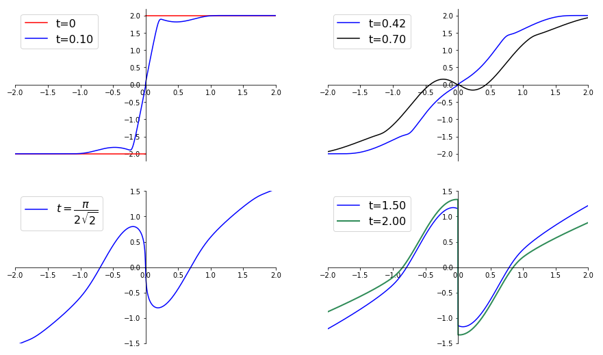
Refer to caption
Figure 4.4: Evolution in time of (a numerical approximation of) the solution uu to (CL)–(4.1)–(5.29), constructed in Theorem 4.1, as a function of the space variable xx, computed at different times, see also Figure 1.1. Note the initial rarefaction profile turning into a shock at time T=π/(22)T=\left.\pi\middle/(2\sqrt{2})\right..

5 Proofs

Several results of use below can be obtained through rather classical techniques but can hardly be precisely localized in the literature. In these cases, we refer to [32], where all details are provided.

Proof of Lemma 2.2.  Let uo∈ITC​L​(w)u_{o}\in I^{CL}_{T}(w). Call UoU_{o} a primitive of uou_{o}, so that ∂xSTH​J​Uo=w\partial_{x}S^{HJ}_{T}U_{o}=w by [16, Theorem 2.20]. Then, by [10, Theorem 5.3.8], (t,x)↦(StH​J​Uo)​(x)(t,x)\mapsto(S^{HJ}_{t}U_{o})(x) is locally semiconcave in the sense of [10, Definition 1.1.1]. Thus, (t,x)↦(StC​L​uo)​(x)(t,x)\mapsto(S^{CL}_{t}u_{o})(x) is locally one sided Lipschitz continuous in the space variable and hence in 𝐁𝐕𝐥𝐨𝐜​(ℝ,ℝ)\mathbf{BV}_{\mathbf{loc}}(\mathbb{R};\mathbb{R}), for all t>0t>0. As is well known, this ensures the existence of left and right traces at any point of the map x↦(StC​L​uo)​(x)x\mapsto(S^{CL}_{t}u_{o})(x), for all t>0t>0.   □\square

Proof of Proposition 2.4.  It is immediate to prove that (1) implies (2.4). Thanks to (1) and (1), we can use [32, Lemma 8.1.3 and Corollary 8.1.4] which ensure that there exists a function ϕ∈𝐂0​(ℝ+,ℝ)\phi\in\mathbf{C}^{0}(\mathbb{R}_{+};\mathbb{R}) that verifies

∀(x,p)∈ℝ2,H(x,p)≥ϕ(|p|) with ϕ⁡(r)r⟶r→+∞+∞.\forall(x,p)\in\mathbb{R}^{2},\quad H(x,p)\geq\phi\left({\left|p\right|}\right)\quad\mbox{ with }\quad\frac{\phi(r)}{r}{\ \underset{r\to+\infty}{\longrightarrow}\ }+\infty\,. (5.1)

Then, (2.4) readily follows.   □\square

5.1 Proof of Theorem 3.1

Lemma 5.1.

Let HH satisfy (C3), (1) and (1). Fix Uo∈𝐋𝐢𝐩⁡(ℝ,ℝ)U_{o}\in\mathbf{Lip}(\mathbb{R};\mathbb{R}) and let UU solve (1) in the sense of Definition 2.3. Fix T>0T>0 and ξ,ζ∈𝐋𝐢𝐩⁡([0,T],ℝ)\xi,\zeta\in\mathbf{Lip}([0,T];\mathbb{R}), with ξ≤ζ\xi\leq\zeta. Then for all s,τ∈[0,T]s,\tau\in[0,T] with s<τs<\tau,

∫ξ⁡(τ)ζ⁡(τ)U⁡(τ,x)​d​x−∫ξ⁡(s)ζ⁡(s)U⁡(s,x)​d​x+∫sτ∫ξ⁡(t)ζ⁡(t)H⁡(x,∂xU⁡(t,x))​d​x​d​t\displaystyle\int_{\xi(\tau)}^{\zeta(\tau)}U(\tau,x)\mathinner{\mathrm{d}{x}}-\int_{\xi(s)}^{\zeta(s)}U(s,x)\mathinner{\mathrm{d}{x}}+\int_{s}^{\tau}\int_{\xi(t)}^{\zeta(t)}H\left(x,\partial_{x}U(t,x)\right)\mathinner{\mathrm{d}{x}}\mathinner{\mathrm{d}{t}} (5.2)
=∫sτ(ζ˙​(t)​U​(t,ζ⁡(t))−ξ˙​(t)​U​(t,ξ⁡(t)))​d​t.\displaystyle=\int_{s}^{\tau}\left(\dot{\zeta}(t)\,U\left(t,\zeta(t)\right)-\dot{\xi}(t)\,U\left(t,\xi(t)\right)\right)\mathinner{\mathrm{d}{t}}.

This Lemma is analogous to [20, Lemma 3.2], see [32, Lemma 8.3.13] for a detailed proof.

Proof of Theorem 3.1.  We only prove the result for the maximal backward characteristic ζ^\hat{\zeta}, which we denote for simplicity ζ\zeta. The details of the proof for the minimal characteristic ζˇ\check{\zeta} are similar.

Fix ε>0\varepsilon>0. Apply Lemma 5.1 with ζ\zeta and ξ=ζ−ε\xi=\zeta-\varepsilon on [0,t][0,t] and s=0s=0, τ=t\tau=t. After dividing by ε\varepsilon, we obtain:

1ε​∫ζ⁡(t)−εζ⁡(t)U⁡(t,y)​d​y−1ε​∫ζ⁡(0)−εζ⁡(0)Uo​(y)​d​y+1ε​∫0t∫ζ⁡(s)−εζ⁡(s)H⁡(y,∂xU⁡(s,y))​d​y​d​s\displaystyle\frac{1}{\varepsilon}\int_{\zeta(t)-\varepsilon}^{\zeta(t)}U(t,y)\mathinner{\mathrm{d}{y}}-\frac{1}{\varepsilon}\int_{\zeta(0)-\varepsilon}^{\zeta(0)}U_{o}(y)\mathinner{\mathrm{d}{y}}+\frac{1}{\varepsilon}\int_{0}^{t}\int_{\zeta(s)-\varepsilon}^{\zeta(s)}H\left(y,\partial_{x}U(s,y)\right)\mathinner{\mathrm{d}{y}}\mathinner{\mathrm{d}{s}} (5.3)
=1ε​∫0tζ˙​(s)​(U⁡(s,ζ⁡(s))−U⁡(s,ζ⁡(s)−ε))​d​s.\displaystyle=\frac{1}{\varepsilon}\int_{0}^{t}\dot{\zeta}(s)\left(U\left(s,\zeta(s)\right)-U\left(s,\zeta(s)-\varepsilon\right)\right)\mathinner{\mathrm{d}{s}}.

We want to pass to the limit ε→0\varepsilon\to 0 in (5.3). To this aim, recall that U⁡(t,⋅)U(t,\cdot) and UoU_{o} are continuous in xx by Definition 2.3. Moreover, ∂xU\partial_{x}U solves (CL) in the sense of Definition 2.1 with initial data Uo′U_{o}^{\prime}, see [16, Theorem 2.20]. For a.e. s∈[0,t]s\in[0,t], ∂xU⁡(s,⋅)\partial_{x}U(s,\cdot) has left and right limits at x=ζ⁡(s)x=\zeta(s) that exist by Lemma 2.2 and coincide, since ζ\zeta is genuine [20, Definition 3.2 and Theorem 3.2]. The map UU is Lipschitz continuous, hence U⁡(s,x2)−U⁡(s,x1)=∫x1x2∂xU⁡(s,y)​d​yU(s,x_{2})-U(s,x_{1})=\int_{x_{1}}^{x_{2}}\partial_{x}U(s,y)\,\mathinner{\mathrm{d}{y}}, so that for a.e. s∈[0,t]s\in[0,t], U⁡(s,⋅)U(s,\cdot) is differentiable at x=ζ⁡(s)x=\zeta(s) and ∂xU⁡(s,ζ⁡(s))=limh→0∂xU⁡(s,ζ⁡(s)+h)\partial_{x}U\left(s,\zeta(s)\right)=\lim_{h\to 0}\partial_{x}U(s,\zeta(s)+h). We thus obtain:

U⁡(t,ζ⁡(t))−Uo​(ζ⁡(0))=∫0t(ζ˙​(s)​∂xU⁡(s,ζ⁡(s))−H⁡(ζ⁡(s),∂xU⁡(s,ζ⁡(s))))​d​s.U\left(t,\zeta(t)\right)-U_{o}\left(\zeta(0)\right)=\int_{0}^{t}\left(\dot{\zeta}(s)\,\partial_{x}U\left(s,\zeta(s)\right)-H\left(\zeta(s),\partial_{x}U\left(s,\zeta(s)\right)\right)\right)\mathinner{\mathrm{d}{s}}. (5.4)

Since ζ\zeta is genuine, there exists a function ω∈𝐂1(]0,t[;ℝ)\omega\in\mathbf{C}^{1}(\mathopen{]}0,t\mathclose{[};\mathbb{R}) such that (ζ,ω)(\zeta,\omega) is a solution to system (HS) with final conditions ζ⁡(t)=x\zeta(t)=x and ω⁡(t)=∂xU⁡(t,x+)\omega(t)=\partial_{x}U(t,x+), since ζ\zeta is a maximal characteristics, see [20, Theorem 3.3]. Moreover, for a.e. s∈[0,t]s\in[0,t], ω⁡(s)=∂xU⁡(s,ζ⁡(s))\omega(s)=\partial_{x}U\left(s,\zeta(s)\right). Combining these details with (5.4) and (1), classical computations lead to:

U⁡(t,x)−Uo​(ζ⁡(0))\displaystyle U(t,x)-U_{o}\left(\zeta(0)\right) =∫0t(ζ˙​(s)​ω​(s)−H⁡(ζ⁡(s),ω⁡(s)))​d​s\displaystyle=\int_{0}^{t}\left(\dot{\zeta}(s)\;\omega(s)-H\left(\zeta(s),\omega(s)\right)\right)\mathinner{\mathrm{d}{s}}
=∫0t(∂pH⁡(ξ⁡(s),ω⁡(s))​ω​(s)−H⁡(ζ⁡(s),ω⁡(s)))​d​s\displaystyle=\int_{0}^{t}\left(\partial_{p}H\left(\xi(s),\omega(s)\right)\,\omega(s)-H\left(\zeta(s),\omega(s)\right)\right)\mathinner{\mathrm{d}{s}}
=∫0tL⁡(ζ⁡(s),∂pH⁡(ξ⁡(s),ω⁡(s)))​d​s\displaystyle=\int_{0}^{t}L\left(\zeta(s),\partial_{p}H\left(\xi(s),\omega(s)\right)\right)\mathinner{\mathrm{d}{s}}
=∫0tL⁡(ζ⁡(s),ζ˙​(s))​d​s,\displaystyle=\int_{0}^{t}L\left(\zeta(s),\dot{\zeta}(s)\right)\mathinner{\mathrm{d}{s}}\,,

concluding the proof.   □\square

Further information about the regularity of UU along characteristics can be found in [10, § 5.5].

5.2 Proof of Theorem 3.2

In the light of the regularity proved in Lemma 2.2, whenever w∈𝐋∞​(ℝ,ℝ)w\in\mathbf{L}^{\infty}(\mathbb{R};\mathbb{R}) is such that ITC​L​(w)≠∅I_{T}^{CL}(w)\neq\emptyset, then by w⁡(x)w(x), we mean the left trace w⁡(x−)w(x-) of ww at xx, for all x∈ℝx\in\mathbb{R}.

Lemma 5.2.

Let HH satisfy (C3), (1) and (1). Then, for all (qo,po)∈ℝ2(q_{o},p_{o})\in\mathbb{R}^{2}, the Cauchy problem (HS) with initial datum (qo,po)(q_{o},p_{o}) at time 00 admits a unique maximal solution (q,p)(q,p) defined on all ℝ\mathbb{R} and satisfying, with the notation (2.4),

|p⁡(t)|≤sup|u|≤|po|x∈ℝ|H⁡(x,u)|+sup|v|≤1x∈ℝL⁡(x,v).{\left|p(t)\right|}\leq\sup_{\begin{subarray}{c}{\left|u\right|}\leq{\left|p_{o}\right|}\\ x\in\mathbb{R}\end{subarray}}{\left|H(x,u)\right|}+\sup_{\begin{subarray}{c}{\left|v\right|}\leq 1\\ x\in\mathbb{R}\end{subarray}}L(x,v)\,. (5.5)

Moreover, calling (q,p)(q,p) the solution to (HS) with datum (qo,po)(q_{o},p_{o}) at time 00, the maps

ℱ:ℝ3⟶ℝ2(t,qo,po)⟼(q⁡(t),p⁡(t))ℱq:ℝ3⟶ℝ(t,qo,po)⟼q⁡(t)ℱp:ℝ3⟶ℝ(t,qo,po)⟼p⁡(t)\!\!\!\!\!\!\!\begin{array}[]{l@{\,}ccc}\mathcal{F}\colon&\mathbb{R}^{3}&\longrightarrow&\mathbb{R}^{2}\\ &\displaystyle{(t,q_{o},p_{o})}&\longmapsto&\displaystyle{\left(q(t),p(t)\right)}\end{array}\;\begin{array}[]{l@{\,}ccc}\mathcal{F}_{q}\colon&\mathbb{R}^{3}&\longrightarrow&\mathbb{R}\\ &\displaystyle{(t,q_{o},p_{o})}&\longmapsto&\displaystyle{q(t)}\end{array}\;\begin{array}[]{l@{\,}ccc}\mathcal{F}_{p}\colon&\mathbb{R}^{3}&\longrightarrow&\mathbb{R}\\ &\displaystyle{(t,q_{o},p_{o})}&\longmapsto&\displaystyle{p(t)}\end{array}\!\! (5.6)

are of class 𝐂2\mathbf{C}^{2}.

Proof of Lemma 5.2.  By (C3), the standard Cauchy Lipschitz Theorem ensures local existence and uniqueness of a solution (q,p)(q,p) to the Cauchy problem for (HS) with datum (qo,po)(q_{o},p_{o}). Moreover, since HH is conserved along solutions to (HS), for all tt where (q,p)(q,p) is defined,

sup|u|≤|po|x∈ℝ|H⁡(x,u)|≥H⁡(qo,po)=H⁡(q⁡(t),p⁡(t))≥|p⁡(t)|−sup|v|≤1x∈ℝL⁡(x,v),\sup_{\begin{subarray}{c}{\left|u\right|}\leq{\left|p_{o}\right|}\\ x\in\mathbb{R}\end{subarray}}{\left|H(x,u)\right|}\geq H(q_{o},p_{o})=H\left(q(t),p(t)\right)\geq{\left|p(t)\right|}-\sup_{\begin{subarray}{c}{\left|v\right|}\leq 1\\ x\in\mathbb{R}\end{subarray}}L(x,v)\,,

where we used (2.4), see also [32, Formula (8.1.5)] with λ=1\lambda=1, proving (5.5). By (HS), (C3) and (5.5), we also have that the solution (q,p)(q,p) is bounded and uniformly continuous on bounded intervals. Hence, it is globally defined.

Standard results on ordinary differential equations, see e.g. [9, Theorem 3.9, Theorem 3.10], ensure that the flow ℱ\mathcal{F} is as regular as ∂qH\partial_{q}H, ∂xH\partial_{x}H and, by (C3), the proof is completed.   □\square

The next three lemmas state in full rigor simple geometric properties that are consequences of (1) and (1) on the graph of HH (essentially, a canyon along the xx direction).

Lemma 5.3.

Let HH satisfy (C3), (1) and (1). Then, there exists a unique function

z:ℝ⟶ℝx⟼z⁡(x) such that ∀x∈ℝ∂pH(x,z(x))=0.\begin{array}[]{l@{\,}ccc}z\colon&\mathbb{R}&\longrightarrow&\mathbb{R}\\ &\displaystyle{x}&\longmapsto&\displaystyle{z(x)}\end{array}\quad\mbox{ such that }\quad\forall\,x\in\mathbb{R}\quad\partial_{p}H\left(x,z(x)\right)=0\,. (5.7)

Moreover, z∈𝐂2​(ℝ,ℝ)z\in\mathbf{C}^{2}(\mathbb{R};\mathbb{R}), if |x|≥X{\left|x\right|}\geq X then z′​(x)=0z^{\prime}(x)=0 and the following quantities are well defined

z¯≔minx∈ℝ⁡z⁡(x),z¯≔maxx∈ℝ⁡z⁡(x),𝐊≔maxx∈ℝ⁡H⁡(x,z⁡(x)).\underline{z}\coloneqq\min_{x\in\mathbb{R}}z(x)\,,\qquad\overline{z}\coloneqq\max_{x\in\mathbb{R}}z(x)\,,\qquad\mathbf{K}\coloneqq\max_{x\in\mathbb{R}}H\left(x,z(x)\right)\,. (5.8)

Proof of Lemma 5.3.  Existence and uniqueness of zz follow from (1). Together, (C3) and (1) allow to apply the Implicit Function Theorem, proving both the 𝐂2\mathbf{C}^{2} regularity of zz and, by (1), that z′​(x)=0z^{\prime}(x)=0 whenever |x|≥X{\left|x\right|}\geq X. The completion of the proof is now immediate.   □\square

Lemma 5.4.

Let HH satisfy (C3), (1) and (1). Referring to the function zz and to the constant 𝐊\mathbf{K} defined in Lemma 5.3, there exist functions

m:ℝ×]𝐊,+∞[⟶ℝ(x,c)⟼m⁡(x,c) and M:ℝ×]𝐊,+∞[⟶ℝ(x,c)⟼M⁡(x,c)\begin{array}[]{l@{\,}ccc}m\colon&\mathbb{R}\times\mathopen{]}\mathbf{K},+\infty\mathclose{[}&\longrightarrow&\mathbb{R}\\ &\displaystyle{(x,c)}&\longmapsto&\displaystyle{m(x,c)}\end{array}\quad\mbox{ and }\quad\begin{array}[]{l@{\,}ccc}M\colon&\mathbb{R}\times\mathopen{]}\mathbf{K},+\infty\mathclose{[}&\longrightarrow&\mathbb{R}\\ &\displaystyle{(x,c)}&\longmapsto&\displaystyle{M(x,c)}\end{array} (5.9)

uniquely characterized, for c>𝐊c>\mathbf{K} and x∈ℝx\in\mathbb{R}, by

H⁡(x,m⁡(x,c))=c and m⁡(x,c)<z⁡(x)H⁡(x,M⁡(x,c))=c and M⁡(x,c)>z⁡(x)\begin{array}[]{c}H\left(x,m(x,c)\right)=c\quad\mbox{ and }\quad m(x,c)<z(x)\\ H\left(x,M(x,c)\right)=c\quad\mbox{ and }\quad M(x,c)>z(x)\end{array} (5.10)

Moreover,

  1. (i)

    m,M∈𝐂1(ℝ×]𝐊,+∞[;ℝ)m,M\in\mathbf{C}^{1}(\mathbb{R}\times\mathopen{]}\mathbf{K},+\infty\mathclose{[};\mathbb{R}).

  2. (ii)

    mm and MM have a compact space dependency:

    |x|>X​ and ​c>𝐊⟹∂xm⁡(x,c)=0​ and ​∂xM⁡(x,c)=0.{\left|x\right|}>X\mbox{ and }c>\mathbf{K}\implies\partial_{x}m(x,c)=0\text{ and }\partial_{x}M(x,c)=0\,. (5.11)
  3. (iii)

    For all x∈ℝx\in\mathbb{R}, m⁡(x,⋅)m(x,\cdot) is decreasing while M⁡(x,⋅)M(x,\cdot) is increasing.

  4. (iv)

    For all x∈ℝx\in\mathbb{R}, limc→+∞m⁡(x,c)=−∞\lim_{c\to+\infty}m(x,c)=-\infty and limc→+∞M⁡(x,c)=+∞\lim_{c\to+\infty}M(x,c)=+\infty.

Proof of Lemma 5.4.  We only prove the results for MM, the details for mm are entirely similar.

Assumption (1) ensures that condition (5.10) uniquely defines the map MM in (5.9). An application of the Implicit Function Theorem shows the regularity, by (C3), proving (i).

Again, by the Implicit Function Theorem and the chain rule, we have

∂xH⁡(x,M⁡(x,c))+∂xM⁡(x,c)​∂pH⁡(x,M⁡(x,c))=0,\partial_{x}H\left(x,M(x,c)\right)+\partial_{x}M(x,c)\;\partial_{p}H\left(x,M(x,c)\right)=0\,,

which implies (5.11) by (1) and by (5.9) and (5.10), proving (ii).

By the definitions (5.7) of zz and (5.9)–(5.10) of MM, we have that for all (x,c)∈ℝ×]𝐊,+∞[(x,c)\in\mathbb{R}\times\mathopen{]}\mathbf{K},+\infty\mathclose{[}, M⁡(x,c)>z⁡(x)M(x,c)>z(x) and hence ∂pH⁡(x,M⁡(x,c))>0\partial_{p}H\left(x,M(x,c)\right)>0. Again using the Implicit Function Theorem, ∂cM⁡(x,c)​∂pH⁡(x,M⁡(x,c))=1\partial_{c}M(x,c)\;\partial_{p}H\left(x,M(x,c)\right)=1 proving that ∂cM⁡(x,c)>0\partial_{c}M(x,c)>0, proving (iii).

Since MM is increasing, limc→+∞M⁡(x,c)=supc>𝐊M⁡(x,c)\lim_{c\to+\infty}M(x,c)=\sup_{c>\mathbf{K}}M(x,c). The boundedness of c↦M⁡(x,c)c\mapsto M(x,c) for some xx then contradicts the equality H⁡(x,M⁡(x,c))=cH\left(x,M(x,c)\right)=c, proving (iv).   □\square

Lemma 5.5.

Let HH satisfy (C3), (1) and (1). Referring to the constant 𝐊\mathbf{K} in Lemma 5.3 and to the functions m,Mm,M in Lemma 5.4, define the functions:

v:]𝐊,+∞[⟶ℝc⟼supx∈ℝ∂pH⁡(x,m⁡(x,c)) and V:]𝐊,+∞[⟶ℝc⟼infx∈ℝ∂pH⁡(x,M⁡(x,c))\begin{array}[]{l@{\,}ccc}v\colon&\mathopen{]}\mathbf{K},+\infty\mathclose{[}&\longrightarrow&\mathbb{R}\\ &\displaystyle{c}&\longmapsto&\displaystyle{\sup_{x\in\mathbb{R}}\partial_{p}H\left(x,m(x,c)\right)}\end{array}\;\mbox{ and }\;\begin{array}[]{l@{\,}ccc}V\colon&\mathopen{]}\mathbf{K},+\infty\mathclose{[}&\longrightarrow&\mathbb{R}\\ &\displaystyle{c}&\longmapsto&\displaystyle{\inf_{x\in\mathbb{R}}\partial_{p}H\left(x,M(x,c)\right)}\end{array}

Then:

  1. (i)

    vv is nonincreasing and VV is nondecreasing;

  2. (ii)

    limc→+∞v⁡(c)=−∞\lim_{c\to+\infty}v(c)=-\infty and limc→+∞V⁡(c)=+∞\lim_{c\to+\infty}V(c)=+\infty.

Proof of Lemma 5.5.  By (1) and (ii) in Lemma 5.4, vv and VV are well-defined. We now prove the statements (i) and (ii) for VV, the case of vv being entirely analogous.

From the monotonicity of MM and ∂pH\partial_{p}H with respect to their second argument:

∀x∈ℝ,∀c1,c2>𝐊, if ​c1<c2​ then ​∂pH⁡(x,M⁡(x,c1))≤∂pH⁡(x,M⁡(x,c2)).\forall\,x\in\mathbb{R},\;\forall\,c_{1},c_{2}>\mathbf{K},\;\mbox{ if }c_{1}<c_{2}\mbox{ then }\partial_{p}H\left(x,M(x,c_{1})\right)\leq\partial_{p}H\left(x,M(x,c_{2})\right).

Taking the infimum over x∈ℝx\in\mathbb{R} we prove (i).

By (i), limc→+∞V⁡(c)=supc>𝐊V⁡(c)\lim_{c\to+\infty}V(c)=\sup_{c>\mathbf{K}}V(c). By contradiction, assume that V¯≔supc>𝐊V⁡(c)\overline{V}\coloneqq\sup_{c>\mathbf{K}}V(c) is finite. By the definition of VV and (1),

∀n∈ℕ∩]𝐊,+∞[∃xn∈[−X,X], such that ∂pH(xn,M(xn,n))≤V¯.\forall\,n\in\mathbb{N}\cap\mathopen{]}\mathbf{K},+\infty\mathclose{[}\quad\exists\,x_{n}\in[-X,X],\quad\mbox{ such that }\quad\partial_{p}H\left(x_{n},M(x_{n},n)\right)\leq\overline{V}\,. (5.12)

Up to a subsequence, we can assume that (xn)n(x_{n})_{n} converges to some x¯∈[−X,X]\overline{x}\in[-X,X]. Item (iv) in Lemma 5.4 and (1) imply that limn→+∞∂pH⁡(x¯,M⁡(x¯,n))=+∞\lim_{n\to+\infty}\partial_{p}H\left(\overline{x},M(\overline{x},n)\right)=+\infty. Therefore,

∃N∈ℕ∩]𝐊,+∞[ such that ∀n≥N,∂pH(x¯,M(x¯,n))>V¯.\exists\,N\in\mathbb{N}\cap\mathopen{]}\mathbf{K},+\infty\mathclose{[}\quad\mbox{ such that }\quad\forall\,n\geq N,\quad\partial_{p}H\left(\overline{x},M(\overline{x},n)\right)>\overline{V}\,. (5.13)

The monotonicity of MM and (1), combined with (5.12), result in:

∀n≥N,∂pH⁡(xn,M⁡(xn,N))≤V¯\forall n\geq N,\quad\partial_{p}H\left(x_{n},M(x_{n},N)\right)\leq\overline{V}

which contradicts (5.13), proving (ii).   □\square

Lemma 5.6.

Let HH satisfy (C3), (1) and (1). Fix qo∈ℝq_{o}\in\mathbb{R} and T∈ℝT\in\mathbb{R}. Then, the map p↦ℱq​(T,qo,p)p\mapsto\mathcal{F}_{q}(T,q_{o},p) defined in (5.6) is surjective, in the sense that

∀qT∈ℝ,∃p∗∈ℝ such that ℱq(T,qo,p∗)=qT,\forall\,q_{T}\in\mathbb{R},\quad\exists\,p_{*}\in\mathbb{R}\quad\mbox{ such that }\quad\mathcal{F}_{q}(T,q_{o},p_{*})=q_{T}\,, (5.14)

or, with the notation (2.1),

∀(xo,xT)∈ℝ2,∃q∈ℛT such that q(0)=xo and q(T)=xT.\forall\,(x_{o},x_{T})\in\mathbb{R}^{2},\quad\exists\,q\in\mathcal{R}_{T}\quad\mbox{ such that }\quad q(0)=x_{o}\mbox{ and }q(T)=x_{T}\,. (5.15)

Proof of Lemma 5.6.  Recall the map zz and the scalar 𝐊\mathbf{K} defined in Lemma 5.3. Fix co>𝐊c_{o}>\mathbf{K} and let po=M⁡(qo,co)p_{o}=M(q_{o},c_{o}). By the conservation of HH, for all t∈ℝt\in\mathbb{R} we have H⁡(ℱq​(t,qo,po),ℱp​(t,qo,po))=coH\left(\mathcal{F}_{q}(t,q_{o},p_{o}),\mathcal{F}_{p}(t,q_{o},p_{o})\right)=c_{o}. Hence, by the definition (5.8) of 𝐊\mathbf{K}, for all t∈ℝt\in\mathbb{R}, it follows that ℱp​(t,qo,po)≠z⁡(ℱq​(t,qo,po))\mathcal{F}_{p}(t,q_{o},p_{o})\neq z\left(\mathcal{F}_{q}(t,q_{o},p_{o})\right).

Using the continuity of ℱ\mathcal{F}, proved in Lemma 5.2, as well as the fact that po>z⁡(qo)p_{o}>z(q_{o}), we deduce that

∀t∈ℝ,ℱp​(t,qo,po)>z⁡(ℱq​(t,qo,po)).\forall t\in\mathbb{R},\quad\mathcal{F}_{p}(t,q_{o},p_{o})>z\left(\mathcal{F}_{q}(t,q_{o},p_{o})\right)\,.

Therefore, for all t∈ℝt\in\mathbb{R}, ℱp​(t,qo,po)=M⁡(ℱq​(t,qo,po),co)\mathcal{F}_{p}(t,q_{o},p_{o})=M\left(\mathcal{F}_{q}(t,q_{o},p_{o}),c_{o}\right), as defined in (5.9)–(5.10). Thus, by (HS) and the definition of VV in Lemma 5.5, we have:

ℱq​(T,qo,po)=qo+∫0Tq˙​(s)​d​s≥qo+V⁡(co)​T​⟶co→+∞+∞.\mathcal{F}_{q}(T,q_{o},p_{o})=q_{o}+\int_{0}^{T}\dot{q}(s)\mathinner{\mathrm{d}{s}}\geq q_{o}+V(c_{o})\,T{\ \underset{c_{o}\to+\infty}{\longrightarrow}\ }+\infty\,.

A similar argument, with po=m⁡(qo,co)p_{o}=m(q_{o},c_{o}), yields ℱq​(T,qo,po)≤qo+v⁡(co)​T​⟶co→+∞−∞\mathcal{F}_{q}(T,q_{o},p_{o})\leq q_{o}+v(c_{o})\,T{\ \underset{c_{o}\to+\infty}{\longrightarrow}\ }-\infty. The continuity of ℱq\mathcal{F}_{q} coupled with the Intermediate Value Theorem concludes the proof of Lemma 5.6.   □\square

Lemma 5.7.

Let HH satisfy (C3), (1) and (1). Fix T>0T>0 and W∈𝐋𝐢𝐩⁡(ℝ,ℝ)W\in\mathbf{Lip}(\mathbb{R};\mathbb{R}) such that ITH​J​(W)≠∅I_{T}^{HJ}(W)\neq\emptyset. Then, for all Uo∈ITH​J​(W)U_{o}\in I_{T}^{HJ}(W), with the notation (3.1),

∀x∈ℝ,Uo​(x)≥Uo∗​(x).\forall x\in\mathbb{R},\quad U_{o}(x)\geq U_{o}^{*}(x). (5.16)

Proof of Lemma 5.7.  Fix x∈ℝx\in\mathbb{R} and y∈ℛTy\in\mathcal{R}_{T} so that y⁡(0)=xy(0)=x. Since Uo∈ITH​J​(W)U_{o}\in I_{T}^{HJ}(W), by (2.5) we have:

W⁡(y⁡(T))−∫0TL⁡(y⁡(s),y˙​(s))​d​s\displaystyle W\left(y(T)\right)-\int_{0}^{T}L\left(y(s),\dot{y}(s)\right)\mathinner{\mathrm{d}{s}}
=\displaystyle= infγ⁡(T)=y⁡(T)γ∈ℛT(∫0TL⁡(γ⁡(s),γ˙​(s))​d​s+Uo​(γ⁡(0)))−∫0TL⁡(y⁡(s),y˙​(s))​d​s\displaystyle\inf_{\begin{subarray}{c}\gamma(T)=y(T)\\ \gamma\in\mathcal{R}_{T}\end{subarray}}\left(\int_{0}^{T}L\left(\gamma(s),\dot{\gamma}(s)\right)\mathinner{\mathrm{d}{s}}+U_{o}\left(\gamma(0)\right)\right)-\int_{0}^{T}L\left(y(s),\dot{y}(s)\right)\mathinner{\mathrm{d}{s}}
≤\displaystyle\leq ∫0TL⁡(y⁡(s),y˙​(s))​d​s+Uo​(y⁡(0))−∫0TL⁡(y⁡(s),y˙​(s))​d​s\displaystyle\int_{0}^{T}L\left(y(s),\dot{y}(s)\right)\mathinner{\mathrm{d}{s}}+U_{o}\left(y(0)\right)-\int_{0}^{T}L\left(y(s),\dot{y}(s)\right)\mathinner{\mathrm{d}{s}}
≤\displaystyle\leq Uo​(y​(0))\displaystyle U_{o}\left(y(0)\right)
=\displaystyle= Uo​(x).\displaystyle U_{o}(x)\,.

By taking the supremum over y∈ℛTy\in\mathcal{R}_{T}, by (3.1) we complete the proof.   □\square

By the second condition in (5.1), for any W∈𝐋𝐢𝐩⁡(ℝ,ℝ)W\in\mathbf{Lip}(\mathbb{R};\mathbb{R}), there exists 𝐂H,W>0\mathbf{C}_{H,W}>0 such that

∀r∈ℝ+,r≥𝐂H,W⟹ϕ⁡(r)1+r>(sup|p|≤‖W′‖𝐋∞​(ℝ,ℝ)q∈ℝ|H⁡(q,p)|+sup|v|≤1q∈ℝ|L⁡(q,v)|),\forall r\in\mathbb{R}_{+},\;r\geq\mathbf{C}_{H,W}\implies\frac{\phi(r)}{1+r}>\biggl(\sup_{\begin{subarray}{c}{\left|p\right|}\leq{\left\|W^{\prime}\right\|}_{\mathbf{L}^{\infty}(\mathbb{R};\mathbb{R})}\\ q\in\mathbb{R}\end{subarray}}{\left|H(q,p)\right|}+\sup_{\begin{subarray}{c}{\left|v\right|}\leq 1\\ q\in\mathbb{R}\end{subarray}}{\left|L(q,v)\right|}\biggr), (5.17)
Lemma 5.8.

Let HH satisfy (C3), (1) and (1). Fix T>0T>0 and W∈𝐋𝐢𝐩⁡(ℝ,ℝ)W\in\mathbf{Lip}(\mathbb{R};\mathbb{R}). Then, Uo∗U_{o}^{*} defined by (3.1) is Lipschitz continuous and

‖(Uo∗)′‖𝐋∞​(ℝ,ℝ)≤T⁡(sup|v|≤𝐂H,Wx∈ℝ|∂xL⁡(x,v)|+‖W′‖𝐋∞​(ℝ,ℝ)).{\left\|(U_{o}^{*})^{\prime}\right\|}_{\mathbf{L}^{\infty}(\mathbb{R};\mathbb{R})}\leq T\biggl(\sup_{\begin{subarray}{c}{\left|v\right|}\leq\mathbf{C}_{H,W}\\ x\in\mathbb{R}\end{subarray}}{\left|\partial_{x}L(x,v)\right|}+{\left\|W^{\prime}\right\|}_{\mathbf{L}^{\infty}(\mathbb{R};\mathbb{R})}\biggr)\,. (5.18)

Moreover, in its definition (3.1), the sup\sup is attained and for any Hamiltonian ray qq realizing the maximum in (3.1), ‖q˙‖𝐋∞​([0,T],ℝ)≤𝐂H,W{\left\|\dot{q}\right\|}_{\mathbf{L}^{\infty}([0,T];\mathbb{R})}\leq\mathbf{C}_{H,W}.

Proof of Lemma 5.8.  First, thanks to (3.1), remark that

∀x∈ℝ,−Uo∗​(x)=infq⁡(0)=xq∈ℛT(∫0TL⁡(q⁡(s),q˙​(s))​d​s−W⁡(q⁡(T))).\forall x\in\mathbb{R},\quad-U_{o}^{*}(x)=\inf_{\begin{subarray}{c}q(0)=x\\ q\in\mathcal{R}_{T}\end{subarray}}\left(\int_{0}^{T}L\left(q(s),\dot{q}(s)\right)\mathinner{\mathrm{d}{s}}-W\left(q(T)\right)\right).

Now reverse time applying the change of variable τ≔T−s\tau\coloneqq T-s and introducing qr​(τ)≔q⁡(T−τ)q^{r}(\tau)\coloneqq q(T-\tau), Lr​(x,v)≔L⁡(x,−v)L^{r}(x,v)\coloneqq L(x,-v), Hr​(x,p)≔supv∈ℝ(p​v−Lr​(x,v))H^{r}(x,p)\coloneqq\sup_{v\in\mathbb{R}}\left(p\,v\ -L^{r}(x,v)\right) so that Hr​(x,p)=H⁡(x,−p)H^{r}(x,p)=H(x,-p). Moreover, using pr​(τ)=−p⁡(T−τ)p^{r}(\tau)=-p(T-\tau), q∈ℛTq\in\mathcal{R}_{T} if and only if qr∈ℛTrq^{r}\in\mathcal{R}^{r}_{T}, where ℛTr\mathcal{R}^{r}_{T} is the set of Hamiltonian rays (2.1) defined by HrH^{r}, with reversed time.

∀x∈ℝ,−Uo∗​(x)=infqr​(T)=xqr∈ℛTr(∫0TLr​(qr​(τ),q˙r​(τ))​d​τ−W⁡(qr​(0))).\forall x\in\mathbb{R},\quad-U_{o}^{*}(x)=\inf_{\begin{subarray}{c}q^{r}(T)=x\\ q^{r}\in\mathcal{R}^{r}_{T}\end{subarray}}\left(\int_{0}^{T}L^{r}\left(q^{r}(\tau),\dot{q}^{r}(\tau)\right)\mathinner{\mathrm{d}{\tau}}-W\left(q^{r}(0)\right)\right)\,.

Then, in view of [32, Corollary 8.3.15],

∀x∈ℝ,−Uo∗​(x)=infqr​(T)=xqr∈𝐋𝐢𝐩⁡([0,T],ℝ)(∫0TLr​(qr​(τ),q˙r​(τ))​d​τ−W⁡(qr​(0))).\forall x\in\mathbb{R},\quad-U_{o}^{*}(x)=\inf_{\begin{subarray}{c}q^{r}(T)=x\\ q^{r}\in\mathbf{Lip}([0,T];\mathbb{R})\end{subarray}}\left(\int_{0}^{T}L^{r}\left(q^{r}(\tau),\dot{q}^{r}(\tau)\right)\mathinner{\mathrm{d}{\tau}}-W\left(q^{r}(0)\right)\right)\,. (5.19)

So that, by [32, Theorem 8.3.12], −Uo∗​(x)=Ur​(T,x)-U_{o}^{*}(x)=U^{r}(T,x), with UrU^{r} being the viscosity solution to the Hamilton-Jacobi equation

{∂tUr+Hr​(x,∂xUr)=0U~​(0,x)=−W​(x),\left\{\begin{array}[]{l}\partial_{t}U^{r}+H^{r}(x,\partial_{x}U^{r})=0\\ \tilde{U}(0,x)=-W(x)\,,\end{array}\right.

proving (5.18).

The result in [32, Corollary 8.3.15] ensures that the supremum in Definition (3.1) is attained as a maximum. We can now combine [32, Theorem 8.3.9] and [32, Corollary 8.3.15] to complete the proof.   □\square

Remarkably, the next Lemma does not require WW to be reachable.

Lemma 5.9.

Let HH satisfy (C3), (1) and (1). Fix T>0T>0 and W∈𝐋𝐢𝐩⁡(ℝ,ℝ)W\in\mathbf{Lip}(\mathbb{R};\mathbb{R}). Then 𝒢\mathcal{G}, as defined in (3.2) has the following properties.

  1. (i)

    𝒢\mathcal{G} is surjective in the following sense:

    ∀xo∈ℝ,∃xT∈ℝ,(xo,xT)∈𝒢.\forall x_{o}\in\mathbb{R},\;\exists x_{T}\in\mathbb{R},\quad(x_{o},x_{T})\in\mathcal{G}. (5.20)
  2. (ii)

    𝒢\mathcal{G} is a closed subset of ℝ2\mathbb{R}^{2}.

  3. (iii)

    For all (xo,xT)∈𝒢(x_{o},x_{T})\in\mathcal{G}, we have

    |xo−xT|≤T​𝐂H,W.{\left|x_{o}-x_{T}\right|}\leq T\,\mathbf{C}_{H,W}\,. (5.21)
  4. (iv)

    𝒢\mathcal{G} is monotone in the following sense:

    ∀(xo,xT),(yo,yT)∈𝒢,xo<yo⟹xT≤yT;xT<yT⟹xo≤yo.\forall\,(x_{o},x_{T}),(y_{o},y_{T})\in\mathcal{G},\quad\begin{array}[]{r@{\,}c@{\,}l@{\implies}r@{\,}c@{\,}l}x_{o}&<&y_{o}&x_{T}&\leq&y_{T}\,;\\ x_{T}&<&y_{T}&x_{o}&\leq&y_{o}\,.\end{array} (5.22)

It is worth noting the connection between (iv) and [15, Lemma 8.1], inspired by [29, Lemma 2.2], see also [26, Sections 5 and 6]. However, the xx dependence makes the present proof significantly different and more intricate.

Proof of Lemma 5.9.  Consider the different items separately.

Property (5.20) comes from the definition of Uo∗U_{o}^{*}, since the sup\sup is actually a max\max by Lemma 5.8.

Proof of (ii):

Let (xon,xTn)n(x_{o}^{n},x_{T}^{n})_{n} be a sequence taking values in 𝒢\mathcal{G} which converges to some (xo,xT)∈ℝ2(x_{o},x_{T})\in\mathbb{R}^{2}. By definition, for all n∈ℕn\in\mathbb{N}, there exists qn∈ℛTq^{n}\in\mathcal{R}_{T} such that

xon=qn​(0),xTn=qn​(T),Uo∗​(xon)=W⁡(xTn)−∫0TL⁡(qn​(s),q˙n​(s))​d​s.x_{o}^{n}=q^{n}(0),\quad x_{T}^{n}=q^{n}(T),\quad U_{o}^{*}(x_{o}^{n})=W(x_{T}^{n})-\int_{0}^{T}L\left(q^{n}(s),\dot{q}^{n}(s)\right)\mathinner{\mathrm{d}{s}}\,. (5.23)

For all n∈ℕn\in\mathbb{N}, let us denote by pn∈𝐂1​([0,T],ℝ)p^{n}\in\mathbf{C}^{1}([0,T];\mathbb{R}) a curve associated with qnq^{n}, given by (xon,xTn)∈𝒢(x_{o}^{n},x_{T}^{n})\in\mathcal{G}. Lemma 5.8 ensures that for all n∈ℕn\in\mathbb{N}, ‖q˙n‖𝐋∞​(]0,T[,ℝ)≤𝐂H,W{\left\|\dot{q}^{n}\right\|}_{\mathbf{L}^{\infty}(]0,T[;\mathbb{R})}\leq\mathbf{C}_{H,W}. Note that for all n∈ℕn\in\mathbb{N}, qn∈𝐂1​([0,T],ℝ)q^{n}\in\mathbf{C}^{1}([0,T];\mathbb{R}) by (2.1). Thanks to (1) and (2.4),

q˙n​(t)=∂pH⁡(qn​(t),pn​(t))⇔pn​(t)=∂vL⁡(qn​(t),q˙n​(t)).\dot{q}^{n}(t)=\partial_{p}H\left(q^{n}(t),p^{n}(t)\right)\iff p^{n}(t)=\partial_{v}L\left(q^{n}(t),\dot{q}^{n}(t)\right)\,.

This proves the boundedness of (pn​(0))\left(p^{n}(0)\right) and, up to a subsequence, we can assume that (pn​(0),qn​(0))n\left(p^{n}(0),q^{n}(0)\right)_{n} converges to (po,xo)(p_{o},x_{o}) with po∈ℝp_{o}\in\mathbb{R}. By Lemma 5.2, the flow of the Hamiltonian system is continuous and we establish the existence of (q,p)∈𝐂0​([0,T],ℝ2)(q,p)\in\mathbf{C}^{0}([0,T];\mathbb{R}^{2}) such that (qn)n(q^{n})_{n} and (pn)n(p^{n})_{n} converge uniformly on [0,T][0,T] to qq and pp, respectively. Using the integral form of (HS), we deduce that (q,p)(q,p) solves (HS). Hence, q∈ℛTq\in\mathcal{R}_{T} and (xo,xT)∈𝒢(x_{o},x_{T})\in\mathcal{G}.

Proof of (iii):

Let (xo,xT)∈𝒢(x_{o},x_{T})\in\mathcal{G} and let q∈ℛTq\in\mathcal{R}_{T} with q⁡(0)=xoq(0)=x_{o} and q⁡(T)=xTq(T)=x_{T}. Then, in view of Lemma 5.8 (latter part), we have

|xo−xT|=|q⁡(0)−q⁡(T)|≤T​‖q˙‖𝐋∞​(]0,T[,ℝ)≤T​𝐂H,W.{\left|x_{o}-x_{T}\right|}={\left|q(0)-q(T)\right|}\leq T\,{\left\|\dot{q}\right\|}_{\mathbf{L}^{\infty}(]0,T[;\mathbb{R})}\leq T\,\mathbf{C}_{H,W}\,.

Proof of (iv):

We only prove the first implication in (5.22), the details of the proof for the second one are similar so we omit them. Let x,y∈ℛTx,y\in\mathcal{R}_{T} be two maximizers for Uo∗​(xo)U_{o}^{*}(x_{o}) and Uo∗​(yo)U_{o}^{*}(y_{o}), respectively. By assumption, we have x⁡(0)<y⁡(0)x(0)<y(0) so that we can define

τ=sup{t∈[0,T]:x⁡(s)<y⁡(s)​ for all ​s∈[0,t]}\tau=\sup\left\{t\in[0,T]\colon x(s)<y(s)\mbox{ for all }s\in[0,t]\right\} (5.24)

and assume, by contradiction, that τ<T\tau<T, so that x⁡(τ)=y⁡(τ)x(\tau)=y(\tau). Define the concatenation

∀t∈[0,T],ξ⁡(t)={y⁡(t)if0≤t≤τ,x⁡(t)ifτ<t≤T.\forall t\in[0,T],\quad\xi(t)=\left\{\begin{array}[]{lcl}y(t)&\text{if}&0\leq t\leq\tau\,,\\ x(t)&\text{if}&\tau<t\leq T\,.\end{array}\right.

Clearly, ξ∈𝐋𝐢𝐩⁡([0,T],ℝ)\xi\in\mathbf{Lip}([0,T];\mathbb{R}) and ξ⁡(0)=yo\xi(0)=y_{o}.

We now prove that x˙​(τ)≠y˙​(τ)\dot{x}(\tau)\neq\dot{y}(\tau). Denote px,py∈𝐂1​([0,T],ℝ)p_{x},p_{y}\in\mathbf{C}^{1}([0,T];\mathbb{R}) the curves associated with xx and yy, respectively, given by (xo,xT),(yo,yT)∈𝒢(x_{o},x_{T}),(y_{o},y_{T})\in\mathcal{G}. Then,

x˙​(τ)=y˙​(τ)\displaystyle\dot{x}(\tau)=\dot{y}(\tau) ⇔∂pH⁡(x⁡(τ),px​(τ))=∂pH⁡(y⁡(τ),py​(τ))\displaystyle\iff\partial_{p}H\left(x(\tau),p_{x}(\tau)\right)=\partial_{p}H\left(y(\tau),p_{y}(\tau)\right)
⇔∂pH⁡(y⁡(τ),px​(τ))=∂pH⁡(y⁡(τ),py​(τ))⇔px​(τ)=py​(τ),\displaystyle\iff\partial_{p}H\left(y(\tau),p_{x}(\tau)\right)=\partial_{p}H\left(y(\tau),p_{y}(\tau)\right)\iff p_{x}(\tau)=p_{y}(\tau)\,,

since p↦∂pH⁡(y⁡(τ),p)p\mapsto\partial_{p}H\left(y(\tau),p\right) is a bijection by (1). However this contradicts the uniqueness of solutions to (HS), see Lemma 5.2.

Hence, ξ\xi is not differentiable at point τ\tau. Moreover, since xx and yy are maximizers, we have, in light of the Dynamic Programming Principle [32, Corollary 8.3.15]:

Uo∗​(xo)−W⁡(xT)\displaystyle U_{o}^{*}(x_{o})-W(x_{T})
=\displaystyle= −infq⁡(0)=xoq∈ℛT∫0TL(q(s),q˙(s))d​s\displaystyle-\inf_{\begin{subarray}{c}q(0)=x_{o}\\ q\in\mathcal{R}_{T}\end{subarray}}\int_{0}^{T}L\left(q(s),\dot{q}(s)\right)\mathinner{\mathrm{d}{s}}
=\displaystyle= −infq⁡(0)=xoq∈𝐋𝐢𝐩(]0,T[;ℝ)∫0TL(q(s),q˙(s))d​s\displaystyle-\inf_{\begin{subarray}{c}q(0)=x_{o}\\ q\in\mathbf{Lip}(\mathopen{]}0,T\mathclose{[};\mathbb{R})\end{subarray}}\int_{0}^{T}L\left(q(s),\dot{q}(s)\right)\mathinner{\mathrm{d}{s}}
=\displaystyle= −infq⁡(0)=xo,q⁡(τ)=ξ⁡(τ)q∈𝐋𝐢𝐩⁡(]0,τ[,ℝ)∫0τL(q(s),q˙(s))d​s−infq⁡(τ)=ξ⁡(τ),q⁡(T)=xTq∈𝐋𝐢𝐩⁡(]τ,T[,ℝ)∫τTL(q(s),q˙(s))d​s\displaystyle-\inf_{\begin{subarray}{c}q(0)=x_{o},q(\tau)=\xi(\tau)\\ q\in\mathbf{Lip}(]0,\tau[;\mathbb{R})\end{subarray}}\int_{0}^{\tau}L\left(q(s),\dot{q}(s)\right)\mathinner{\mathrm{d}{s}}-\inf_{\begin{subarray}{c}q(\tau)=\xi(\tau),q(T)=x_{T}\\ q\in\mathbf{Lip}(]\tau,T[;\mathbb{R})\end{subarray}}\int_{\tau}^{T}L\left(q(s),\dot{q}(s)\right)\mathinner{\mathrm{d}{s}}
=\displaystyle= −∫0τL(y(s),y˙(s))d​s−∫τTL(x(s),x˙(s))d​s\displaystyle-\int_{0}^{\tau}L\left(y(s),\dot{y}(s)\right)\mathinner{\mathrm{d}{s}}-\int_{\tau}^{T}L\left(x(s),\dot{x}(s)\right)\mathinner{\mathrm{d}{s}}
=\displaystyle= −∫0TL(ξ(s),ξ˙(s))d​s.\displaystyle-\int_{0}^{T}L\left(\xi(s),\dot{\xi}(s)\right)\mathinner{\mathrm{d}{s}}\,.

This ensures that ξ\xi is a Lipschitz maximizer for Uo∗​(xo)U_{o}^{*}(x_{o}), therefore, ξ∈𝐖2,∞(]0,T[;ℝ)\xi\in\mathbf{W}^{2,\infty}(\mathopen{]}0,T\mathclose{[};\mathbb{R}) by [32, Corollary 8.3.7]. However, this contradicts the fact that ξ\xi is not differentiable at t=τt=\tau. We conclude that xx and yy do not cross in ]0,T[\mathopen{]}0,T\mathclose{[} implying x⁡(T)≤y⁡(T)x(T)\leq y(T) and, hence, xT≤yTx_{T}\leq y_{T}.   □\square

Proof of Theorem 3.2.  The proof of the implication (1) ⟹\implies (2) is clear.

Proof of (2) ⟹\implies (3).

Suppose that ITH​J​(W)≠∅I_{T}^{HJ}(W)\neq\emptyset and set w=W′w=W^{\prime}, so that ITC​L​(w)≠∅I_{T}^{CL}(w)\neq\emptyset by the correspondence between (CL) and (1) proved in [16, Theorem 2.20]. We check that 𝒢\mathcal{G} in (3.2) enjoys the maximal property (3.3). Fix Uo∈ITH​J​(W)U_{o}\in I_{T}^{HJ}(W), (xo,xT′),(xo,xT′′)∈𝒢(x_{o},x_{T}^{\prime}),(x_{o},x_{T}^{\prime\prime})\in\mathcal{G}, with xT′<xT′′x_{T}^{\prime}<x_{T}^{\prime\prime}, and xT∈]xT′,xT′′[x_{T}\in\mathopen{]}x_{T}^{\prime},x_{T}^{\prime\prime}\mathclose{[}. Let y,z∈ℛTy,z\in\mathcal{R}_{T}, as defined in (2.1), be solutions to (HS) connecting (xo,xT′)(x_{o},x_{T}^{\prime}) and (xo,xT′′)(x_{o},x_{T}^{\prime\prime}), respectively, and let ξ\xi be the minimal backward generalized characteristics emanating from (T,xT)(T,x_{T}), associated with (CL) with initial data Uo′U_{o}^{\prime}. By [20, Theorem 3.2], ξ\xi is genuine, ξ∈ℛT\xi\in\mathcal{R}_{T} and by Theorem 3.1,

W⁡(xT)=∫0TL⁡(ξ⁡(s),ξ˙​(s))​d​s+Uo​(ξ⁡(0))≥∫0TL⁡(ξ⁡(s),ξ˙​(s))​d​s+Uo∗​(ξ⁡(0)).W(x_{T})=\int_{0}^{T}L\left(\xi(s),\dot{\xi}(s)\right)\mathinner{\mathrm{d}{s}}+U_{o}\left(\xi(0)\right)\geq\int_{0}^{T}L\left(\xi(s),\dot{\xi}(s)\right)\mathinner{\mathrm{d}{s}}+U_{o}^{*}\left(\xi(0)\right).

Above, we used the fact that Uo≥Uo∗U_{o}\geq U_{o}^{*}, see Lemma 5.7. We deduce that

Uo∗​(ξ⁡(0))≤W⁡(xT)−∫0TL⁡(ξ⁡(s),ξ˙​(s))​d​s.U_{o}^{*}\left(\xi(0)\right)\leq W(x_{T})-\int_{0}^{T}L\left(\xi(s),\dot{\xi}(s)\right)\mathinner{\mathrm{d}{s}}.

By definition (3.1) of Uo∗U_{o}^{*}, we have equality above, and therefore ξ\xi is a point of maximum of the functional in (3.1). We deduce that (ξ⁡(0),xT)∈𝒢(\xi(0),x_{T})\in\mathcal{G}. By (5.22) in Lemma 5.9,

xT′<xT⟹xo≤ξ⁡(0)andxT′′>xT⟹xo≥ξ⁡(0).x_{T}^{\prime}<x_{T}\implies x_{o}\leq\xi(0)\quad\text{and}\quad x_{T}^{\prime\prime}>x_{T}\implies x_{o}\geq\xi(0).

We deduce that ξ⁡(0)=xo\xi(0)=x_{o} and, therefore, (xo,xT)∈𝒢(x_{o},x_{T})\in\mathcal{G}.

Proof of (3) ⟹\implies (1).

We now show that Uo∗U_{o}^{*}, as defined in (3.1), is in ITH​J​(W)I_{T}^{HJ}(W). We first check that:

∀xT∈ℝ,∃xo∈ℝ,(xo,xT)∈𝒢.\forall\,x_{T}\in\mathbb{R},\;\exists\,x_{o}\in\mathbb{R},\quad(x_{o},x_{T})\in\mathcal{G}. (5.25)

Note that (5.25) differs from (i) in Lemma 5.9, since the roles of the elements in the pair (xo,xT)(x_{o},x_{T}) are reversed.

Fix xT∈ℝx_{T}\in\mathbb{R} and introduce the subset:

E={x∈ℝ:∃y∈]−∞,xT[ and (x,y)∈𝒢}.E=\left\{x\in\mathbb{R}\colon\exists\,y\in\mathopen{]}-\infty,x_{T}\mathclose{[}\mbox{ and }(x,y)\in\mathcal{G}\right\}\,.

Fix x∈ℝx\in\mathbb{R} such that x<xT−T​𝐂H,Wx<x_{T}-T\,\mathbf{C}_{H,W}. As a consequence of (i) in Lemma 5.9, there exists y∈ℝy\in\mathbb{R} such that (x,y)∈𝒢(x,y)\in\mathcal{G}. Now, using (iii) in Lemma 5.9, we can write

y=(y−x)+x<|x−y|+(xT−T​𝐂H,W)≤xT,y=(y-x)+x<{\left|x-y\right|}+(x_{T}-T\,\mathbf{C}_{H,W})\leq x_{T}\,,

which ensures that ]−∞,xT−T𝐂H,W[⊂E\mathopen{]}-\infty,x_{T}-T\,\mathbf{C}_{H,W}\mathclose{[}\subset E and, therefore, EE is non-empty. Moreover, for all x∈Ex\in E, if y∈ℝy\in\mathbb{R} (y<xTy<x_{T}) is such that (x,y)∈𝒢(x,y)\in\mathcal{G}, then we have

x≤(x−y)+y<|x−y|+xT≤T​𝐂H,W+xT,x\leq(x-y)+y<{\left|x-y\right|}+x_{T}\leq T\,\mathbf{C}_{H,W}+x_{T}\,,

proving that EE is bounded above. Hence, x¯=supE\overline{x}=\sup E is finite. Likewise, the subset

F={x∈ℝ:∃y∈]xT,+∞[ and (x,y)∈𝒢}F=\left\{x\in\mathbb{R}\colon\exists\,y\in\mathopen{]}x_{T},+\infty\mathclose{[}\mbox{ and }(x,y)\in\mathcal{G}\right\}

is nonempty and bounded below. Therefore, x¯=infF\underline{x}=\inf F is finite. The monotonicity of 𝒢\mathcal{G} in (iv) of Lemma 5.9 ensures that x¯≤x¯\overline{x}\leq\underline{x}.

Let (xn)n(x_{n})_{n} be a sequence of EE which converges to x¯\overline{x}. For all n∈ℕn\in\mathbb{N}, there exists yn<xTy_{n}<x_{T} such that (xn,yn)∈𝒢(x_{n},y_{n})\in\mathcal{G}. Since (xn)n(x_{n})_{n} is bounded, (yn)n(y_{n})_{n} is bounded as well, as a consequence of (iii) in Lemma 5.9. Up to the extraction of a subsequence, we can assume that (yn)n(y_{n})_{n} converges to some y¯≤xT\overline{y}\leq x_{T}. Since 𝒢\mathcal{G} is closed, by (i) in Lemma 5.9, (x¯,y¯)∈𝒢(\overline{x},\overline{y})\in\mathcal{G}. The same way, there exists y¯≥xT\underline{y}\geq x_{T} such that (x¯,y¯)∈𝒢(\underline{x},\underline{y})\in\mathcal{G}. Let us conclude the proof by a case by case study.

Case 1: x¯=x¯\overline{x}=\underline{x}.

Call xox_{o} this common value. Since y¯≤xT≤y¯\overline{y}\leq x_{T}\leq\underline{y}, we have by (3.3)

(xo,y¯),(xo,y¯)∈𝒢⟹(xo,xT)∈𝒢.(x_{o},\overline{y}),(x_{o},\underline{y})\in\mathcal{G}\implies(x_{o},x_{T})\in\mathcal{G}\,.

Case 2: x¯<x¯\overline{x}<\underline{x}.

Fix xo∈]x¯,x¯[x_{o}\in\mathopen{]}\overline{x},\underline{x}\mathclose{[}. By (i) in Lemma 5.9, there exists y∈ℝy\in\mathbb{R} such that (xo,y)∈𝒢(x_{o},y)\in\mathcal{G}. However, by the definition of x¯\overline{x}, we necessarily have y≥xTy\geq x_{T}. Similarly, the definition of x¯\underline{x} ensures that y≤xTy\leq x_{T}. We proved that y=xTy=x_{T} and therefore, (xo,xT)∈𝒢(x_{o},x_{T})\in\mathcal{G} for any xo∈]x¯,x¯[x_{o}\in\mathopen{]}\overline{x},\underline{x}\mathclose{[}.

Equality (5.25) rewrites as:

∀x∈ℝ,∃q∈ℛT:q⁡(T)=x​ and ​W​(x)=∫0TL⁡(q⁡(s),q˙​(s))​d​s+Uo∗​(q⁡(0)).\forall\,x\in\mathbb{R},\;\exists\,q\in\mathcal{R}_{T}\colon q(T)=x\mbox{ and }W(x)=\int_{0}^{T}L\left(q(s),\dot{q}(s)\right)\mathinner{\mathrm{d}{s}}+U_{o}^{*}\left(q(0)\right)\,. (5.26)

Moreover, by the definition of Uo∗U_{o}^{*}, we also have

∀q∈ℛT∫0TL⁡(q⁡(s),q˙​(s))​d​s+Uo∗​(q⁡(0))≥W⁡(q⁡(T)).\forall\,q\in\mathcal{R}_{T}\qquad\int_{0}^{T}L\left(q(s),\dot{q}(s)\right)\mathinner{\mathrm{d}{s}}+U_{o}^{*}\left(q(0)\right)\geq W\left(q(T)\right)\,. (5.27)

Together (5.26) and (5.27) imply that

∀x∈ℝ,W⁡(x)\displaystyle\forall x\in\mathbb{R},\quad W(x) =infq⁡(T)=xq∈ℛT∫0TL⁡(q⁡(s),q˙​(s))​d​s+Uo∗​(q⁡(0))\displaystyle=\inf_{\begin{subarray}{c}q(T)=x\\ q\in\mathcal{R}_{T}\end{subarray}}\int_{0}^{T}L\left(q(s),\dot{q}(s)\right)\mathinner{\mathrm{d}{s}}+U_{o}^{*}\left(q(0)\right)
=infq⁡(T)=xq∈𝐋𝐢𝐩(]0,T[;ℝ)∫0TL⁡(q⁡(s),q˙​(s))​d​s+Uo∗​(q⁡(0)),\displaystyle=\inf_{\begin{subarray}{c}q(T)=x\\ q\in\mathbf{Lip}(\mathopen{]}0,T\mathclose{[};\mathbb{R})\end{subarray}}\int_{0}^{T}L\left(q(s),\dot{q}(s)\right)\mathinner{\mathrm{d}{s}}+U_{o}^{*}\left(q(0)\right)\,,

by [32, Corollary 8.3.15]. This last equality means that the viscosity solution UU to (1) associated with initial datum Uo∗U_{o}^{*} verifies U⁡(T)=WU(T)=W, using the classical correspondence viscosity solution/calculus of variations, see [32, Theorem 8.3.12]. We proved that Uo∗∈ITH​J​(W)U_{o}^{*}\in I_{T}^{HJ}(W).

Proof of (2) ⟹\implies πW′\pi_{W^{\prime}} is well defined and nondecreasing.

Suppose that ITH​J​(W)≠∅I_{T}^{HJ}(W)\neq\emptyset and set w=W′w=W^{\prime}, so that ITC​L​(w)≠∅I_{T}^{CL}(w)\neq\emptyset by [16, Theorem 2.20]. In the light of both Lemma 2.2 and Lemma 5.2, πw\pi_{w} is well-defined by (2.2).

Fix x,y∈ℝx,y\in\mathbb{R} with x<yx<y. Since ITC​L​(w)≠∅I_{T}^{CL}(w)\neq\emptyset, πw\pi_{w} assigns to xx, respectively yy, the value at time t=0t=0 of the minimal backward generalized characteristics emanating from (T,x)(T,x), respectively from (T,y)(T,y), which we denote by ξx\xi_{x}, respectively ξy\xi_{y}. By [20, Theorem 3.2], ξx\xi_{x} and ξy\xi_{y} are genuine, hence they do not intersect in ]0,T[\mathopen{]}0,T\mathclose{[}, see [20, Corollary 3.2]. This implies in particular that ξx​(0)≤ξy​(0)\xi_{x}(0)\leq\xi_{y}(0), proving that πw\pi_{w} is nondecreasing.   □\square

5.3 Proof of Theorem 3.3

Proof of Theorem 3.3.  We prove the two implications separately.

Claim: If Uo∈ITH​J​(W)U_{o}\in I^{HJ}_{T}(W), then (i) and (ii) hold.

Point (i) comes from Lemma 5.7. Let us prove that (ii) holds. Fix xo∈πW′​(ℝ)x_{o}\in\pi_{W^{\prime}}(\mathbb{R}). By definition, there exists an x∈ℝx\in\mathbb{R} such that xo=πW′​(x)x_{o}=\pi_{W^{\prime}}(x). This means that xox_{o} is the value at time t=0t=0 of the minimal backward characteristics ξ\xi, see [20, Definition 3.1, Theorems 3.2 and 3.3] emanating from (T,x)(T,x). Since Uo∈ITH​J​(W)U_{o}\in I_{T}^{HJ}(W), Theorem 3.1 ensures that

W⁡(x)=∫0TL⁡(ξ⁡(s),ξ˙​(s))​d​s+Uo​(xo).W(x)=\int_{0}^{T}L\left(\xi(s),\dot{\xi}(s)\right)\mathinner{\mathrm{d}{s}}+U_{o}(x_{o})\,.

On the other hand, by (3.1),

Uo∗​(xo)=supy⁡(0)=xoy∈ℛT(W⁡(y⁡(T))−∫0TL⁡(y⁡(s),y˙​(s)))​d​s≥W⁡(x)−∫0TL⁡(ξ⁡(s),ξ˙​(s))​d​s=Uo​(xo).U_{o}^{*}(x_{o})=\sup_{\begin{subarray}{c}y(0)=x_{o}\\ y\in\mathcal{R}_{T}\end{subarray}}\left(W\left(y(T)\right){-}\int_{0}^{T}\!L\left(y(s),\dot{y}(s)\right)\right)\mathinner{\mathrm{d}{s}}\geq W(x)-\int_{0}^{T}\!L\left(\xi(s),\dot{\xi}(s)\right)\mathinner{\mathrm{d}{s}}=U_{o}(x_{o}).

So, Uo=Uo∗U_{o}=U_{o}^{*} on πW′​(ℝ)\pi_{W^{\prime}}(\mathbb{R}). These two functions are continuous, hence they coincide on πW′​(ℝ)¯\overline{\pi_{W^{\prime}}(\mathbb{R})}.

Claim: If (i) and (ii) hold, then Uo∈ITH​J​(W)U_{o}\in I^{HJ}_{T}(W).

Fix x∈ℝx\in\mathbb{R}. Recall that ITH​J​(W)≠∅I_{T}^{HJ}(W)\neq\emptyset which, by Theorem 3.2, ensures that Uo∗∈ITH​J​(W)U_{o}^{*}\in I_{T}^{HJ}(W). This, together with the inequality Uo≥Uo∗U_{o}\geq U_{o}^{*}, immediately implies:

W⁡(x)\displaystyle W(x) =\displaystyle= infy⁡(T)=xy∈ℛT(∫0TL⁡(y⁡(s),y˙​(s))​d​s+Uo∗​(y⁡(0)))\displaystyle\inf_{\begin{subarray}{c}y(T)=x\\ y\in\mathcal{R}_{T}\end{subarray}}\left(\int_{0}^{T}L\left(y(s),\dot{y}(s)\right)\mathinner{\mathrm{d}{s}}+U_{o}^{*}\left(y(0)\right)\right) (5.28)
≤\displaystyle\leq infy⁡(T)=xy∈ℛT(∫0TL⁡(y⁡(s),y˙​(s))​d​s+Uo​(y⁡(0))).\displaystyle\inf_{\begin{subarray}{c}y(T)=x\\ y\in\mathcal{R}_{T}\end{subarray}}\left(\int_{0}^{T}L\left(y(s),\dot{y}(s)\right)\mathinner{\mathrm{d}{s}}+U_{o}\left(y(0)\right)\right).

Denote by ξ\xi the minimal backward characteristics emanating from (T,x)(T,x). Using both the facts that Uo∗∈ITH​J​(W)U_{o}^{*}\in I_{T}^{HJ}(W) and that, by Theorem 3.1, ξ\xi is a minimizer, we have:

W⁡(x)=∫0TL⁡(ξ⁡(s),ξ˙​(s))​d​s+Uo∗​(ξ⁡(0)).W(x)=\int_{0}^{T}L\left(\xi(s),\dot{\xi}(s)\right)\mathinner{\mathrm{d}{s}}+U_{o}^{*}\left(\xi(0)\right).

Clearly, ξ⁡(0)∈πW′​(ℝ)¯\xi(0)\in\overline{\pi_{W^{\prime}}(\mathbb{R})} and therefore, by (ii), we can replace Uo∗​(ξ⁡(0))U_{o}^{*}\left(\xi(0)\right) by Uo​(ξ​(0))U_{o}\left(\xi(0)\right) in the last equality. This ensures that we have equality in (5.28), which means that Uo∈ITH​J​(W)U_{o}\in I_{T}^{HJ}(W).   □\square

5.4 Proof of Theorem 4.1

In all proofs in this section, the reader might want to keep Figure 1.1 in mind for a helpful geometrical visualization.

Long but straightforward computations show that HH, as defined in (4.1), satisfies (C3), (1) with X=1X=1, and (1), see Figure 4.3. With this flux, the conservation law (CL) is also the inviscid Burger equation with source term −g′-g^{\prime}, see Figure 4.3. We fix the initial datum

uo​(x)≔{−2if ​x<0,2if ​x>0,u_{o}(x)\coloneqq\left\{\begin{array}[]{cl}-2&\text{if }x<0\,,\\ 2&\text{if }x>0\,,\end{array}\right. (5.29)

which would evolve into a rarefaction in the homogeneous case. The proof of Theorem 4.1 is based on the Cauchy problem for (HS) which, in this case, reads

{q˙=pp˙=−g′​(q)q⁡(0)=qop⁡(0)=powith ​g​ as in (4.1),\left\{\begin{array}[]{rcl}\dot{q}&=&p\\ \dot{p}&=&-g^{\prime}(q)\\ q(0)&=&q_{o}\\ p(0)&=&p_{o}\end{array}\right.\qquad\mbox{with }g\mbox{ as in~\eqref{eq:11},} (5.30)

and to which Lemma 5.2 applies. The first equation in (5.30) will be tacitly used throughout this section. By the Hamiltonian nature of (5.30), HH is conserved along solutions, so that

∀t∈ℝ,p​(t)22+g⁡(q⁡(t))=po22+g⁡(qo).\forall t\in\mathbb{R},\quad\frac{p(t)^{2}}{2}+g\left(q(t)\right)=\frac{p_{o}^{2}}{2}+g(q_{o})\,. (5.31)
Lemma 5.10.

Let HH be as in (4.1) and uou_{o} be as in (5.29). Fix qo≥0q_{o}\geq 0. Denote by (q,p)(q,p) the solution to (5.30) with initial datum (qo,uo​(qo+))=(qo,2)\left(q_{o},u_{o}(q_{o}+)\right)=(q_{o},2). Then, qq is increasing on [0,+∞[[0,+\infty\mathclose{[} and q⁡(t)​⟶t→+∞+∞q(t){\ \underset{t\to+\infty}{\longrightarrow}\ }+\infty.

Proof of Lemma 5.10.  Note that po>0p_{o}>0. By (5.31), for all t∈ℝt\in\mathbb{R}

p​(t)2=p​(0)2⏟=4+2​g⁡(qo)⏟≥0−2​g⁡(q⁡(t))⏟≤1≥2.p(t)^{2}=\underbrace{{p(0)}^{2}}_{=4}+2\underbrace{g(q_{o})}_{\geq 0}-2\underbrace{g\left(q(t)\right)}_{\leq 1}\geq 2\,.

Thus, for t∈ℝt\in\mathbb{R}, p⁡(t)≥2p(t){\geq}\sqrt{2}. By (HS), qq is strictly increasing and q⁡(t)≥2​tq(t){\geq}\sqrt{2}\,t for t∈[0,+∞[t{\in}[0,+\infty\mathclose{[}.   □\square

Refer to caption
Figure 5.1: On the horizontal axis, the qq component of solutions to (5.30), while tt is on the vertical axis. Brown curves are those considered in (i) of Lemma 5.12; green curves refer to Lemma 5.13. The 2 red thicker curves depict solutions corresponding to the initial data (0,2)(0,\sqrt{2}) and (0,2)(0,2). The black curves are those considered in Lemma 5.10 and in Lemma 5.11.

Refer to the lines on the right in Figure 5.1 for an illustration of the different behaviors of qq described in Lemma 5.10 and Lemma 5.11.

Lemma 5.11.

Let HH be as in (4.1) and uou_{o} be as in (5.29). Fix 0≤qo<qo~0\leq q_{o}<\widetilde{q_{o}} and denote by (q,p)(q,p), respectively (q~,p~)(\widetilde{q},\widetilde{p}), the global solution to (HS) with initial datum (qo,uo​(qo+))=(qo,2)\left(q_{o},u_{o}(q_{o}+)\right)=(q_{o},2), respectively (qo~,uo​(qo~))=(qo~,2)\left(\widetilde{q_{o}},u_{o}(\widetilde{q_{o}})\right)=(\widetilde{q_{o}},2). Then, q​(t)<q~​(t)q(t)<\widetilde{q}(t), for all t≥0t\geq 0.

Proof of Lemma 5.11.  Set po=uo​(qo)p_{o}=u_{o}(q_{o}) and po~=uo​(qo~)\widetilde{p_{o}}=u_{o}(\widetilde{q_{o}}). We proceed by contradiction. Let τ>0\tau>0, be the smallest time where q​(τ)=q~​(τ)q(\tau)=\tilde{q}(\tau). Since qo<q~oq_{o}<\tilde{q}_{o}, we have that p​(τ)≥p~​(τ)p(\tau)\geq\tilde{p}(\tau). By Lemma 5.10, p⁡(τ)≥p~​(τ)≥0p(\tau)\geq\widetilde{p}(\tau)\geq 0. Then,

qo∈[0,qo~[po=p~o}\displaystyle\left.\begin{array}[]{@{}r@{\,}c@{\,}l@{}}q_{o}&\in&[0,\widetilde{q_{o}}\mathclose{[}\\ p_{o}&=&\tilde{p}_{o}\end{array}\right\} ⟹po22+g⁡(qo)≤po~22+g⁡(qo~)\displaystyle\implies\frac{p_{o}^{2}}{2}+g(q_{o})\leq\frac{\widetilde{p_{o}}^{2}}{2}+g(\widetilde{q_{o}}) [By (4.1) and (5.29)]\displaystyle[\mbox{By~\eqref{eq:11} and~\eqref{eq:12}}]
⟹p​(τ)22+g⁡(q⁡(τ))≤p~​(τ)22+g⁡(q~​(τ))\displaystyle\implies\frac{p(\tau)^{2}}{2}+g\left(q(\tau)\right)\leq\frac{\widetilde{p}(\tau)^{2}}{2}+g\left(\widetilde{q}(\tau)\right) [By (5.31)]\displaystyle[\mbox{By~\eqref{eq:conservation_ce}}]
⟹p​(τ)≤p~​(τ).\displaystyle\implies p(\tau)\leq\widetilde{p}(\tau). [By q(τ)=q~(τ),p(τ)≥p~(τ)>0]\displaystyle[\mbox{By }q(\tau)=\widetilde{q}(\tau),\;p(\tau)\geq\widetilde{p}(\tau)>0]

We then deduce that p​(τ)=p~​(τ)p(\tau)=\widetilde{p}(\tau), which contradicts the uniqueness proved by Cauchy Lipschitz Theorem.   □\square

Lemma 5.12.

Let HH be as in (4.1) and uou_{o} be as in (5.29). Fix po∈[2,2[p_{o}\in[\sqrt{2},2\mathclose{[}. Denote by (q,p)(q,p) the global solution to (5.30) with initial datum (0,po)(0,p_{o}). (Refer to Figure 5.1.)

  1. (i)

    If po∈]2,2[p_{o}\in\mathopen{]}\sqrt{2},2\mathclose{[}, then qq is increasing on [0,+∞[[0,+\infty\mathclose{[} and q⁡(t)​⟶t→+∞+∞q(t){\ \underset{t\to+\infty}{\longrightarrow}\ }+\infty.

  2. (ii)

    If po=2p_{o}=\sqrt{2}, then qq is increasing on [0,+∞[[0,+\infty\mathclose{[}, q⁡(t)​⟶t→+∞​ 1q(t){\ \underset{t\to+\infty}{\longrightarrow}\ }1 and qq is concave.

Refer to the middle curves in Figure 5.1 for an illustration of the different behaviors of qq described in Lemma 5.12.

Proof of Lemma 5.12.  The proof of (i) is identical to that of Lemma 5.10, so we omit it.

Concerning (ii), pp is positive on ]0,+∞[\mathopen{]}0,+\infty\mathclose{[}. Indeed, assume by contradiction that there exists a minimal τ>0\tau>0 such that p⁡(τ)=0p(\tau)=0. By (5.31), we deduce that q⁡(τ)=1q(\tau)=1. However, (qs,ps):t↦(1,0)(q_{s},p_{s})\colon t\mapsto(1,0) is the unique global solution to (5.30) with datum (1,0)(1,0). Hence, pp is positive on ]0,+∞[\mathopen{]}0,+\infty\mathclose{[}.

Thus, by (5.30), qq is increasing on [0,+∞[[0,+\infty\mathclose{[} and positive on ]0,+∞[]0,+\infty\mathclose{[}. Once again, (5.31) and the presence of the stationary solution (qs,ps)(q_{s},p_{s}) ensure that for all t∈[0,+∞[t\in[0,+\infty\mathclose{[}, q⁡(t)<1q(t)<1. Therefore, as t→+∞t\to+\infty, qq admits a finite limit, say q∞q_{\infty}, which is not greater than 11.

Moreover, the positivity of qq ensures, by (5.30), that pp is nonincreasing on [0,+∞[[0,+\infty\mathclose{[}, so that by (5.30), qq is concave. Since pp is also bounded, by (5.5) in Lemma 5.2, pp admits a finite limit as t→+∞t\to+\infty. Hence, q˙\dot{q} has a finite limit as t→+∞t\to+\infty and, since we already showed that qq converges to q∞q_{\infty} as t→+∞t\to+\infty, then q˙→0\dot{q}\to 0 and therefore p→0p\to 0 as t→+∞t\to+\infty. By (5.31), we get g⁡(q∞)=1g(q_{\infty})=1, and hence q∞≥1q_{\infty}\geq 1, therefore q∞=1q_{\infty}=1, completing the proof of (ii).   □\square

Lemma 5.13.

Let HH be as in (4.1) and uou_{o} be as in (5.29). Let po∈]0,2[p_{o}\in\mathopen{]}0,\sqrt{2}\mathclose{[}. Denote by (q,p)(q,p) the global solution to (5.30) with initial data (0,po)(0,p_{o}). Then, qq is periodic. Introduce the map

𝒯:]0,2[⟶]0,+∞[po⟼the smallest period of q\begin{array}[]{l@{\,}ccc}\mathcal{T}\colon&\mathopen{]}0,\sqrt{2}\mathclose{[}&\longrightarrow&\mathclose{]}0,+\infty\mathclose{[}\\ &\displaystyle{p_{o}}&\longmapsto&\displaystyle{\text{the smallest period of $q$}}\end{array} (5.32)
  1. (i)

    qq is concave on [0,𝒯⁡(po)/2][0,\mathcal{T}(p_{o})/2].

  2. (ii)

    For all t∈[0,𝒯⁡(po)/2]t\in\left[0,\mathcal{T}(p_{o})/2\right], q⁡(t)=q⁡(𝒯⁡(po)/2−t)q(t)=q\left(\mathcal{T}(p_{o})/2-t\right).

  3. (iii)

    For all t∈[0,𝒯⁡(po)]t\in\left[0,\mathcal{T}(p_{o})\right], q⁡(t)=−q⁡(𝒯⁡(po)−t)q(t)=-q\left(\mathcal{T}(p_{o})-t\right).

  4. (iv)

    qq admits its maximum at 𝒯⁡(po)/4\mathcal{T}(p_{o})/4.

Proof of Lemma 5.13.  Note first that by (5.31), qq is bounded, since for all t∈ℝt\in\mathbb{R}, g⁡(q⁡(t))=po22−(p⁡(t))22≤po22<1g\left(q(t)\right)=\frac{p_{o}^{2}}{2}-\frac{\left(p(t)\right)^{2}}{2}\leq\frac{p_{o}^{2}}{2}<1 and hence |q⁡(t)|<1{\left|q(t)\right|}<1 for all t∈ℝt\in\mathbb{R}.

Assume now, by contradiction, that qq does not vanish on ]0,+∞[\mathopen{]}0,+\infty\mathclose{[}. Since q⁡(0)=0q(0)=0 and q˙​(0)>0\dot{q}(0)>0, we have that for all t∈]0,+∞[t\in\mathopen{]}0,+\infty\mathclose{[}, q⁡(t)>0q(t)>0. Therefore, pp is decreasing on [0,+∞[[0,+\infty\mathclose{[} by (5.30), bounded by (5.31) and thus admits a finite limit as t→+∞t\to+\infty.

Thus, qq is bounded and its derivative q˙=p\dot{q}=p has a finite limit as t→+∞t\to+\infty, hence limt→+∞q˙​(t)=0\lim_{t\to+\infty}\dot{q}(t)=0 and also limt→+∞p⁡(t)=0\lim_{t\to+\infty}p(t)=0. Therefore, by monotonicity, pp is nonnegative on all [0,+∞[[0,+\infty\mathclose{[}. Consequently, qq is nondecreasing and bounded, therefore it admits a finite limit q∞≥0q_{\infty}\geq 0 as t→+∞t\to+\infty. On the one hand, by taking the limit as t→+∞t\to+\infty in (5.31), we get:

g(q∞)=po22∈]0,1[⟹q∞∈]0,1[⟹g′(q∞)≠0.g(q_{\infty})=\frac{p_{o}^{2}}{2}\in\mathopen{]}0,1\mathclose{[}\implies q_{\infty}\in\mathopen{]}0,1\mathclose{[}\implies g^{\prime}(q_{\infty})\neq 0.

On the other hand, p˙​(t)=−g′​(q⁡(t))→−g′​(q∞)\dot{p}(t)=-g^{\prime}\left(q(t)\right)\to-g^{\prime}(q_{\infty}). Moreover, pp has a finite limit as t→+∞t\to+\infty, p˙​(t)→0\dot{p}(t)\to 0. This provides the needed contradiction.

Thus we proved that there exists τ>0\tau>0 such that q⁡(τ)=0q(\tau)=0. As a consequence, the number

τ∗≔sup{t∈]0,+∞[:∀s∈]0,t[,q(s)>0}\tau_{*}\coloneqq\sup\left\{t\in\mathopen{]}0,+\infty\mathclose{[}\colon\forall\,s\in\mathopen{]}0,t\mathclose{[},\;q(s)>0\right\} (5.33)

is well-defined and satisfies q⁡(τ∗)=0{q(\tau_{*})=0}. Note that for t∈]0,τ∗[t\in\mathopen{]}0,\tau_{*}\mathclose{[}, qq is positive, pp is decreasing and hence qq is concave on [0,τ∗][0,\tau_{*}], proving (i) on [0,τ∗][0,\tau_{*}]. Furthermore, p⁡(τ∗)<pop(\tau_{*})<p_{o}. Apply (5.31) at time t=τ∗t=\tau_{*} to obtain p​(τ∗)2=po2p(\tau_{*})^{2}=p_{o}^{2}, which implies p⁡(τ∗)=−pop(\tau_{*})=-p_{o}.

Now we verify that qq is 2​τ∗2\tau_{*}–periodic. To this aim, introduce ξ⁡(t)=−q⁡(t+τ∗)\xi(t)=-q(t+\tau_{*}) and ν⁡(t)=−p⁡(t+τ∗)\nu(t)=-p(t+\tau_{*}). Thanks to gg being even, it is straightforward to check that both (q,p)(q,p) and (ξ,ν)(\xi,\nu) solve the same Cauchy problem (5.30). Consequently,

∀t∈ℝq⁡(t+2​τ∗)=−q⁡(t+τ∗)=q⁡(t).\forall\,t\in\mathbb{R}\qquad q(t+2\tau_{*})=-q(t+\tau_{*})=q(t)\,. (5.34)

Hence, qq is 2​τ∗2\tau_{*}–periodic. By (5.33), 2​τ∗2\tau_{*} is the minimal period, completing the proof of (i).

Finally, define q^​(t)=q⁡(τ∗−t)\widehat{q}(t)=q(\tau_{*}-t) and p^​(t)=−p⁡(τ∗−t)\widehat{p}(t)=-p(\tau_{*}-t). Note that (q,p)(q,p) and (q^,p^)(\widehat{q},\widehat{p}) both solve (5.30) with datum (0,po)(0,p_{o}), since p⁡(τ∗)=−pop(\tau_{*})=-p_{o}. Hence, for all t∈[0,τ∗]t\in[0,\tau_{*}], q⁡(t)=q⁡(τ∗−t)q(t)=q(\tau_{*}-t), proving (ii). Combined with the concavity of qq, this ensures that maxt∈[0,τ∗]⁡q⁡(t)=q⁡(τ∗/2)\max_{t\in[0,\tau_{*}]}q(t)=q(\tau_{*}/2), proving (iv). Finally, (5.34) and (ii) imply (iii).   □\square

Lemma 5.14.

Let HH be as in (4.1) and uou_{o} be as in (5.29). Call 𝒯\mathcal{T} the map defined in (5.32). Then:

  1. (i)

    𝒯\mathcal{T} is continuous.

  2. (ii)

    𝒯\mathcal{T} strictly increasing.

  3. (iii)

    infpo∈]0,2[𝒯(po)=π/2\inf_{p_{o}\in\mathopen{]}0,\sqrt{2}\mathclose{[}}\mathcal{T}(p_{o})=\left.\pi\middle/\sqrt{2}\right..

  4. (iv)

    limpo→2𝒯⁡(po)=+∞\lim_{p_{o}\to\sqrt{2}}\mathcal{T}(p_{o})=+\infty.

Proof of Lemma 5.14. 

Proof of (i).

Fix po∈]0,2[p_{o}\in\mathopen{]}0,\sqrt{2}\mathclose{[} and let qo=0q_{o}=0. Let (q,p)(q,p) be the solution to (5.30). Then, by Lemma (5.13), we get p​(t)=q˙​(t)>0p(t)=\dot{q}(t)>0 for all t∈]0,𝒯(po)/4[t\in\mathopen{]}0,\mathcal{T}(p_{o})/4\mathclose{[}. Hence, using (5.31) we get

∀t∈]0,𝒯(po)/4[p(t)=po2−2​g​(q⁡(t))\forall\,t\in\mathopen{]}0,\mathcal{T}(p_{o})/4\mathclose{[}\qquad p(t)=\sqrt{p_{o}^{2}-2g\left(q(t)\right)}

and by (5.30), we have

𝒯⁡(po)4=∫0𝒯⁡(po)/4q˙​(t)po2−2​g​(q⁡(t))​d​t.\frac{\mathcal{T}(p_{o})}{4}=\int_{0}^{\mathcal{T}(p_{o})/4}\frac{\dot{q}(t)}{\sqrt{p_{o}^{2}-2g\left(q(t)\right)}}\mathinner{\mathrm{d}{t}}\,. (5.35)

Note that the integrand in the right hand side above is singular when t=𝒯⁡(po)/4t=\mathcal{T}(p_{o})/4, but it is positive for all tt. Use the change of variable x=q⁡(t)x=q(t) to get

𝒯⁡(po)4=∫0g−1​(po2/2)1po2−2​g​(x)​d​x\frac{\mathcal{T}(p_{o})}{4}=\int_{0}^{g^{-1}(p_{o}^{2}/2)}\frac{1}{\sqrt{p_{o}^{2}-2g(x)}}\mathinner{\mathrm{d}{x}} (5.36)

where g−1g^{-1} is the inverse of the 𝐂1\mathbf{C}^{1} diffeomorphism g|]0,1[:]0,1[→]0,1[g_{|\mathopen{]}0,1\mathopen{[}}\colon\mathopen{]}0,1\mathopen{[}\to\mathopen{]}0,1\mathopen{[}.

Define 𝒜:]0,1[→ℝ+\mathcal{A}\colon\mathopen{]}0,1\mathopen{[}\to\mathbb{R}_{+} by

𝒜⁡(r)≔∫01rg⁡(r)−g⁡(θ​r)​d​θ,\mathcal{A}(r)\coloneqq\int_{0}^{1}\dfrac{r}{\sqrt{g(r)-g(\theta\,r)}}\mathinner{\mathrm{d}{\theta}}\,, (5.37)

so that the change of variable x=θ​rx=\theta\,r with r=g−1​(po2/2)r=g^{-1}(p_{o}^{2}/2) in (5.36) leads to

𝒯⁡(po)=2​2​𝒜​(g−1​(po2/2)).\mathcal{T}(p_{o})=2\sqrt{2}\;\mathcal{A}\left(g^{-1}(p_{o}^{2}/2)\right)\,. (5.38)

The continuity of 𝒜\mathcal{A} is proved in Lemma A.2 in Appendix A, completing the proof of (i).

Proof of (ii).

By [11, Theorem A], (5.38) and (5.31), the condition

∀x∈]0,1[,d2d​x2(g⁡(x)g′​(x)2)≥0\forall x\in\mathopen{]}0,1\mathclose{[},\quad\frac{\mathinner{\mathrm{d}{}}^{2}~}{\mathinner{\mathrm{d}{x}}^{2}}\left(\frac{g(x)}{g^{\prime}(x)^{2}}\right)\geq 0

ensures that E↦2​2​𝒜​(g−1​(E))E\mapsto 2\sqrt{2}\,\mathcal{A}\left(g^{-1}(E)\right) is increasing. Hence, by (5.38), also 𝒯\mathcal{T} is increasing on ]0,2[\mathopen{]}0,\sqrt{2}\mathclose{[}. By (4.1), for x∈]0,1[x\in\mathopen{]}0,1\mathclose{[} we have

d2d​x2​(g⁡(x)g′​(x)2)=−332​7​x8−32​x6+59​x4−56​x2−6(x2−1)8.\frac{\mathinner{\mathrm{d}{}}^{2}~}{\mathinner{\mathrm{d}{x}}^{2}}\left(\frac{g(x)}{g^{\prime}(x)^{2}}\right)=-\frac{3}{32}\frac{7x^{8}-32x^{6}+59x^{4}-56x^{2}-6}{(x^{2}-1)^{8}}\,.

We leave to Lemma A.1 in Appendix A the proof that d2d​x2​(g⁡(x)g′​(x)2)≥0\frac{\mathinner{\mathrm{d}{}}^{2}~}{\mathinner{\mathrm{d}{x}}^{2}}\left(\frac{g(x)}{g^{\prime}(x)^{2}}\right)\geq 0 for all x∈]0,1[x\in\mathopen{]}0,1\mathclose{[} by means of Sturm Theorem, see [31].

Proof of (iii).

To prove the lower bound on 𝒯\mathcal{T}, introduce for any po∈]0,2[p_{o}\in\mathopen{]}0,\sqrt{2}\mathclose{[}, q~>0\tilde{q}>0 so that g⁡(q~)=po2/2g(\tilde{q})=p_{o}^{2}/2:

infpo∈]0,2]𝒯(po)\displaystyle\inf_{p_{o}\in]0,\sqrt{2}]}\mathcal{T}(p_{o}) =limpo→0+𝒯⁡(po)\displaystyle=\lim_{p_{o}\to 0+}\mathcal{T}(p_{o}) [By the monotonicity of 𝒯]\displaystyle[\mbox{By the monotonicity of $\mathcal{T}$}]
=limE→02​2​𝒜​(g−1​(E))\displaystyle=\lim_{E\to 0}2\sqrt{2}\;\mathcal{A}\left(g^{-1}(E)\right) [By (5.38)]\displaystyle[\mbox{By~\eqref{eq:27}}]
=limr→02​2​𝒜​(r)\displaystyle=\lim_{r\to 0}2\sqrt{2}\;\mathcal{A}(r) [By (4.1)]\displaystyle[\mbox{By~\eqref{eq:11}}]
=2​2​limr→0∫01rg⁡(r)−g⁡(θ​r)​d​θ\displaystyle=2\sqrt{2}\lim_{r\to 0}\int_{0}^{1}\frac{r}{\sqrt{g(r)-g(\theta\,r)}}\mathinner{\mathrm{d}{\theta}} [By (5.37)]\displaystyle[\mbox{By~\eqref{eq:26}}]
=4​∫01d​θg′′​(0)​(1−θ2)\displaystyle=4\int_{0}^{1}\frac{\mathinner{\mathrm{d}{\theta}}}{\sqrt{g^{\prime\prime}(0)\,(1-\theta^{2})}}
=π2.\displaystyle=\frac{\pi}{\sqrt{2}}\,.

This completes the proof of (iii).

Proof of (iv).

Similar computations, using now Fatou’s Lemma, lead to

limpo→2𝒯⁡(po)=2​2​limr→1∫01rg⁡(r)−g⁡(θ​r)​d​θ≥2​2​∫011(1−θ2)2​d​θ=+∞,\lim_{p_{o}\to\sqrt{2}}\mathcal{T}(p_{o})=2\sqrt{2}\lim_{r\to 1}\int_{0}^{1}\frac{r}{\sqrt{g(r)-g(\theta\,r)}}\mathinner{\mathrm{d}{\theta}}\geq 2\sqrt{2}\int_{0}^{1}\frac{1}{(1-\theta^{2})^{2}}\mathinner{\mathrm{d}{\theta}}=+\infty\,,

completing the proof of (iv) and of Lemma 5.12.   □\square

Lemma 5.15.

Let HH be as in (4.1) and uou_{o} be as in (5.29). Fix 0<po<po~<20<p_{o}<\widetilde{p_{o}}<2 and denote by (q,p)(q,p), respectively (q~,p~)(\widetilde{q},\widetilde{p}), the global solution to (5.30) with initial datum (0,po)(0,p_{o}), respectively (0,po~)(0,\widetilde{p_{o}}). Then,

(i)po∈]0,2[⟹∀t∈]0,𝒯(po)/2]q⁡(t)<q~​(t);(i​i)po∈[2,2[⟹∀t∈]0,+∞[q⁡(t)<q~​(t).\begin{array}[]{c@{\quad}r@{\,}c@{\,}lcr@{\,}c@{\,}l@{\qquad}r@{\,}c@{\,}l}(i)&p_{o}&\in&\mathopen{]}0,\sqrt{2}\mathclose{[}&\implies&\forall\,t&\in&\mathopen{]}0,\mathcal{T}(p_{o})/2]&q(t)&<&\widetilde{q}(t)\,;\\ (ii)&p_{o}&\in&[\sqrt{2},2\mathclose{[}&\implies&\forall\,t&\in&\mathopen{]}0,+\infty\mathclose{[}&q(t)&<&\widetilde{q}(t)\,.\end{array}

Refer to the middle and left curves in Figure 5.1 for an illustration of the different behaviors of qq described in Lemma 5.15.

Proof of Lemma 5.15.  We split the proof in several steps.

Claim 1: Let T>0T>0 be such that p⁡(t)>0p(t)>0 and p~​(t)>0\widetilde{p}(t)>0 for all t∈[0,T]t\in[0,T]. Then, for all t∈[0,T]t\in[0,T], q​(t)<q~​(t)q(t)<\widetilde{q}(t).

By contradiction, since po<p~op_{o}<\widetilde{p}_{o}, there exists s∈]0,T]s\in\mathopen{]}0,T] such that q​(t)<q~​(t)q(t)<\widetilde{q}(t) for t∈]0,s[t\in\mathopen{]}0,s\mathclose{[}, q​(s)=q~​(s)q(s)=\widetilde{q}(s) and thus p​(s)≥p~​(s)p(s)\geq\widetilde{p}(s). Then, by (5.31),

0<po<p~o\displaystyle 0<p_{o}<\widetilde{p}_{o} ⟹H⁡(0,po)<H⁡(0,p~o)\displaystyle\implies H(0,p_{o})<H(0,\widetilde{p}_{o}) [By (4.1)]\displaystyle[\mbox{By~\eqref{eq:11}}]
⟹H⁡(q⁡(s),p⁡(s))<H⁡(q~​(s),p~​(s))\displaystyle\implies H\left(q(s),p(s)\right)<H\left(\widetilde{q}(s),\widetilde{p}(s)\right) [By (5.31)]\displaystyle[\mbox{By~\eqref{eq:conservation_ce}}]
⟹p​(s)<p~​(s)\displaystyle\implies p(s)<\widetilde{p}(s) [Since q(s)=q~(s) and p(s)>0,p~(s)>0]\displaystyle[\mbox{Since }q(s)=\widetilde{q}(s)\mbox{ and }p(s)>0,\;\widetilde{p}(s)>0]

which yields a contradiction, proving Claim 1.

Claim 2: (i) holds for p~o∈]0,2[\widetilde{p}_{o}\in\mathopen{]}0,\sqrt{2}\mathclose{[}.

By Claim 1, for all t∈]0,𝒯(po)/4[t\in\mathopen{]}0,\mathcal{T}(p_{o})/4\mathclose{[}, q​(t)<q~​(t)q(t)<\widetilde{q}(t). Indeed, by (5.30) together with Lemma 5.13 and Lemma 5.14, both pp and p~\widetilde{p} are positive on ]0,𝒯(po)/4[\mathopen{]}0,\mathcal{T}(p_{o})/4\mathclose{[} and Claim 1 applies. Hence, by the symmetry in (ii) of Lemma 5.13, we have

∀t∈]𝒯⁡(p~o)2−𝒯⁡(po)4,𝒯⁡(p~o)2[q(𝒯⁡(p~o)2−t)<q~(t).\forall\ t\in\left]\frac{\mathcal{T}(\widetilde{p}_{o})}{2}-\frac{\mathcal{T}(p_{o})}{4},\frac{\mathcal{T}(\widetilde{p}_{o})}{2}\right[\qquad q\left(\frac{\mathcal{T}(\widetilde{p}_{o})}{2}-t\right)<\widetilde{q}(t)\,.

Introduce the concave function

η:[0,𝒯⁡(p~o)2]⟶ℝt⟼{q⁡(t)t∈[0,𝒯⁡(po)4]q⁡(𝒯⁡(po)4)t∈]𝒯⁡(po)4,𝒯⁡(p~o)2−𝒯⁡(po)4[q⁡(𝒯⁡(p~o)2−t)t∈[𝒯⁡(p~o)2−𝒯⁡(po)4,𝒯⁡(p~o)2]\begin{array}[]{l@{\,}ccc}\eta\colon&\left[0,\frac{\mathcal{T}(\widetilde{p}_{o})}{2}\right]&\longrightarrow&\mathbb{R}\\ &\displaystyle{t}&\longmapsto&\displaystyle{\left\{\begin{array}[]{l@{\qquad}r@{\,}c@{\,}l}q(t)&t&\in&\left[0,\frac{\mathcal{T}(p_{o})}{4}\right]\\[6.0pt] q\left(\frac{\mathcal{T}(p_{o})}{4}\right)&t&\in&\left]\frac{\mathcal{T}(p_{o})}{4},\frac{\mathcal{T}(\widetilde{p}_{o})}{2}-\frac{\mathcal{T}(p_{o})}{4}\right[\\[6.0pt] q\left(\frac{\mathcal{T}(\widetilde{p}_{o})}{2}-t\right)&t&\in&\left[\frac{\mathcal{T}(\widetilde{p}_{o})}{2}-\frac{\mathcal{T}(p_{o})}{4},\frac{\mathcal{T}(\widetilde{p}_{o})}{2}\right]\end{array}\right.}\end{array} (5.39)

and note that, see Figure 5.2,

Refer to caption
Figure 5.2: Curves used in Claim 2 in the proof of Lemma 5.15. The dashed curve is the graph of η\eta in (5.39). The continuous curves are the graphs of qq restricted to [0,𝒯⁡(po)/2][0,\mathcal{T}(p_{o})/2] and of its translate. The dashed–dotted curved is the graph of q~\widetilde{q}.
∀t∈[0,𝒯⁡(po)4]q⁡(t)≤η⁡(t)[By (5.39)]∀t∈[0,𝒯⁡(p~o)2]η⁡(t)≤q~​(t)[By concavity of η and q~]∀t∈[𝒯⁡(po)4,𝒯⁡(po)2]q⁡(t)≤η⁡(t)[By symmetry]\begin{array}[]{r@{\,}c@{\,}l@{\qquad}r@{\,}c@{\,}l@{\qquad}l}\forall\,t&\in&\left[0,\frac{\mathcal{T}(p_{o})}{4}\right]&q(t)&\leq&\eta(t)&[\mbox{By~\eqref{eq:16}}]\\[6.0pt] \forall\,t&\in&\left[0,\frac{\mathcal{T}(\widetilde{p}_{o})}{2}\right]&\eta(t)&\leq&\widetilde{q}(t)&[\mbox{By concavity of $\eta$ and $\widetilde{q}$}]\\[6.0pt] \forall\,t&\in&\left[\frac{\mathcal{T}(p_{o})}{4},\frac{\mathcal{T}(p_{o})}{2}\right]&q(t)&\leq&\eta(t)&[\mbox{By symmetry}]\end{array}

completing the proof of Claim 2.

Claim 3: (i) holds for p~o∈[2,+∞[\widetilde{p}_{o}\in[\sqrt{2},+\infty\mathclose{[}.

By Claim 1, for all t∈]0,𝒯(po)/4]t\in\mathopen{]}0,\mathcal{T}(p_{o})/4\mathclose{]}, q​(t)<q~​(t)q(t)<\widetilde{q}(t).

By (iv) in Lemma 5.13, for all t∈]0,𝒯(po)/2[t\in\mathopen{]}0,\mathcal{T}(p_{o})/2\mathclose{[}, q⁡(t)≤q⁡(𝒯⁡(po)/4)q(t)\leq q(\mathcal{T}(p_{o})/4), while by (i) and (ii) in Lemma 5.12, for p~o∈[2,+∞[\widetilde{p}_{o}\in[\sqrt{2},+\infty\mathclose{[} and for all t∈[𝒯(po)/4,+∞[t\in[\mathcal{T}(p_{o})/4,+\infty\mathclose{[}, q~​(t)>q~​(𝒯⁡(po)/4)\widetilde{q}(t)>\widetilde{q}(\mathcal{T}(p_{o})/4). All this ensures that

∀t∈[𝒯⁡(po)4,𝒯⁡(po)2]q⁡(t)≤q⁡(𝒯⁡(po)4)<q~​(𝒯⁡(po)4)≤q~​(t),\forall\,t\in\left[\frac{\mathcal{T}(p_{o})}{4},\frac{\mathcal{T}(p_{o})}{2}\right]\qquad q(t)\leq q\left(\frac{\mathcal{T}(p_{o})}{4}\right)<\widetilde{q}\left(\frac{\mathcal{T}(p_{o})}{4}\right)\leq\widetilde{q}(t)\,,

completing the proof of Claim 3.

Claim 4: Proof of (ii).

If po,po~∈[2,2[p_{o},\widetilde{p_{o}}\in[\sqrt{2},2[, then by (i) and (ii) in Lemma 5.12, qq and q~\widetilde{q} are increasing, so that by (5.30) pp and p~\widetilde{p} are positive. So, Claim 1 applies, completing the proof.

□\square

We use below the flow ℱ\mathcal{F} introduced in (5.6) with reference to (HS), which we now particularize to (5.30). By Lemma 5.2, ℱ\mathcal{F} is of class 𝐂2\mathbf{C}^{2}. Define

(q♭,p♭)​(t)≔ℱ⁡(t,0,2) and (q♯,p♯)​(t)≔ℱ⁡(t,0,2),(q^{\flat},p^{\flat})(t)\coloneqq\mathcal{F}(t,0,\sqrt{2})\qquad\mbox{ and }\qquad(q^{\sharp},p^{\sharp})(t)\coloneqq\mathcal{F}(t,0,2)\,, (5.40)

q♭q^{\flat}, respectively q♯q^{\sharp}, being the leftmost, respectively rightmost, red line in Figure 5.1.

Lemma 5.16.

Let HH be as in (4.1) and uou_{o} be as in (5.29). Define the set

D≔([0,+∞[×{2})∪({0}×]0,2]).D\coloneqq\left([0,+\infty\mathclose{[}\times\{2\}\right)\cup\left(\{0\}\times\mathopen{]}0,2]\right). (5.41)

Then, there exists a unique map

Δ:]0,+∞[×]0,+∞[⟶D(t,x)⟼(qo,po)\begin{array}[]{l@{\,}ccc}\Delta\colon&\mathopen{]}0,+\infty\mathclose{[}\times\mathopen{]}0,+\infty\mathclose{[}&\longrightarrow&D\\ &\displaystyle{(t,x)}&\longmapsto&\displaystyle{(q_{o},p_{o})}\end{array} (5.42)

such that

ℱq(t,qo,po)=xand∀s∈]0,t[,ℱq(s,qo,po)>0.\mathcal{F}_{q}(t,q_{o},p_{o})=x\quad\text{and}\quad\forall\,s\in\mathopen{]}0,t\mathclose{[},\;\mathcal{F}_{q}(s,q_{o},p_{o})>0\,. (5.43)

Moreover,

  1. (1)

    Δ\Delta is continuous.

  2. (2)

    Δ\Delta is monotone, in the sense that setting Δ⁡(to,xo)=(0,po)\Delta(t_{o},x_{o})=(0,p_{o}) and Δ⁡(to,xo′)=(0,po′)\Delta(t_{o},x_{o}^{\prime})=(0,p_{o}^{\prime}), if 0<xo<xo′<q♯​(to)0<x_{o}<x_{o}^{\prime}<q^{\sharp}(t_{o}), then po<po′p_{o}<p_{o}^{\prime}.

  3. (3)

    For all x∈]0,+∞[x\in\mathopen{]}0,+\infty\mathclose{[}, limt→0+Δ⁡(t,x)=(x,2)\lim_{t\to 0+}\Delta(t,x)=(x,2).

Proof of Lemma 5.16.  We split the proof in several steps.

For all (t,x)∈]0,+∞[2(t,x)\in\mathopen{]}0,+\infty\mathclose{[}^{2}, there exists (po,qo)∈D(p_{o},q_{o})\in D satisfying (5.43).

Fix (t,x)∈]0,+∞[×]0,+∞[(t,x)\in\mathopen{]}0,+\infty\mathclose{[}\times\mathopen{]}0,+\infty\mathclose{[}. If x=q♯​(t)x=q^{\sharp}(t) as in (5.40), then set (qo,po)=(0,2)(q_{o},p_{o})=(0,2). Otherwise, introduce the functions

h:[0,+∞[⟶ℝqo⟼ℱq​(t,qo,2)−x and k:]0,2]⟶ℝpo⟼ℱq​(t,0,po)−x.\begin{array}[]{l@{\,}ccc}h\colon&[0,+\infty\mathclose{[}&\longrightarrow&\mathbb{R}\\ &\displaystyle{q_{o}}&\longmapsto&\displaystyle{\mathcal{F}_{q}(t,q_{o},2)-x}\end{array}\quad\mbox{ and }\quad\begin{array}[]{l@{\,}ccc}k\colon&\mathopen{]}0,2]&\longrightarrow&\mathbb{R}\\ &\displaystyle{p_{o}}&\longmapsto&\displaystyle{\mathcal{F}_{q}(t,0,p_{o})-x\,.}\end{array}

Note that if x>q♯​(t)x>q^{\sharp}(t) then h⁡(0)<0h(0)<0 and h⁡(x+1)=ℱq​(t,x+1,2)−x>0h(x+1)=\mathcal{F}_{q}(t,x+1,2)-x>0 by Lemma 5.10. By the Intermediate Value Theorem, there exists a qoq_{o} such that h⁡(qo)=0h(q_{o})=0, hence ℱq​(t,qo,2)=x\mathcal{F}_{q}(t,q_{o},2)=x. By Lemma 5.10, for all s>0s>0, ℱq​(s,qo,2)>0\mathcal{F}_{q}(s,q_{o},2)>0, proving (5.43) in the case x>q♯​(t)x>q^{\sharp}(t).

If x∈[q♭​(t),q♯​(t)]x\in[q^{\flat}(t),q^{\sharp}(t)], then k⁡(2)≤0≤k⁡(2)k(\sqrt{2})\leq 0\leq k(2) by (5.40). By the Intermediate Value Theorem, there exists pop_{o} such that k⁡(po)=0k(p_{o})=0, i.e., ℱq​(t,0,po)=x\mathcal{F}_{q}(t,0,p_{o})=x. Then, by Lemma 5.15, the right part of (5.43) follows in the case x∈[q♭​(t),q♯​(t)]x\in[q^{\flat}(t),q^{\sharp}(t)].

Similarly, if x∈]0,q♭(t)[x\in\mathopen{]}0,q^{\flat}(t)\mathclose{[}, then k⁡(2)>0k(\sqrt{2})>0 and limpˇ→0+k⁡(pˇ)=−x<0\lim_{\check{p}\to 0+}k(\check{p})=-x<0. By the Intermediate Value Theorem, we can define

po≔max⁡{πo∈[0,2]:k⁡(πo)=0}.p_{o}\coloneqq\max\left\{\pi_{o}\in[0,\sqrt{2}]\colon k(\pi_{o})=0\right\}\,.

Hence, for all pˇ∈]po,2[\check{p}\in\mathopen{]}p_{o},\sqrt{2}\mathclose{[}, k⁡(pˇ)>0k(\check{p})>0. Proceed now by contradiction: assume there exists s∈]0,t[s\in\mathopen{]}0,t\mathclose{[} such that ℱq​(s,0,po)<0\mathcal{F}_{q}(s,0,p_{o})<0. By Lemma 5.13, we get t>𝒯⁡(po)t>\mathcal{T}(p_{o}). Using Lemma 5.14 and the Intermediate Value Theorem, it follows that there exists po′∈]po,2[p_{o}^{\prime}\in\mathopen{]}p_{o},\sqrt{2}\mathclose{[} such that 𝒯⁡(po′)=t\mathcal{T}(p_{o}^{\prime})=t. By Lemma 5.13, this implies that ℱq​(t,0,po′)=0\mathcal{F}_{q}(t,0,p_{o}^{\prime})=0 and therefore k⁡(po′)<0k(p_{o}^{\prime})<0, which contradicts the choice of pop_{o}.

Δ\Delta is uniquely defined.

For all (t,x)∈]0,+∞[×]0,+∞[(t,x)\in\mathopen{]}0,+\infty\mathclose{[}\times\mathopen{]}0,+\infty\mathclose{[} the uniqueness of a (qo,po)(q_{o},p_{o}) satisfying (5.43) follows from the monotonicity properties proved above. Indeed, recalling q♯q^{\sharp} as defined in (5.40), if 0<qo<q~o0<q_{o}<\tilde{q}_{o} and po=p~o=2p_{o}=\tilde{p}_{o}=2, then, by Lemma 5.11, for all s∈[0,+∞[s\in[0,+\infty\mathclose{[}, q♯​(s)<ℱq​(s,qo,po)<ℱq​(s,q~o,p~o)q^{\sharp}(s)<\mathcal{F}_{q}(s,q_{o},p_{o})<\mathcal{F}_{q}(s,\tilde{q}_{o},\tilde{p}_{o}). On the other hand, if qo=q~o=0q_{o}=\tilde{q}_{o}=0 and 0<po<p~o<20<p_{o}<\tilde{p}_{o}<2, then by Lemma 5.12, Lemma 5.13 and Lemma 5.15, for all ss such that ℱq​(τ,qo,po)≥0\mathcal{F}_{q}(\tau,q_{o},p_{o})\geq 0 for all τ∈[0,s]\tau\in[0,s], we have ℱq​(s,qo,po)<ℱq​(s,q~o,p~o)<q♯​(s)\mathcal{F}_{q}(s,q_{o},p_{o})<\mathcal{F}_{q}(s,\tilde{q}_{o},\tilde{p}_{o})<q^{\sharp}(s). Finally, if qo=0q_{o}=0, q~o>0\tilde{q}_{o}>0, po∈]0,2[p_{o}\in\mathopen{]}0,2\mathclose{[} and p~o=2\tilde{p}_{o}=2, then Lemma 5.15 and Lemma 5.11 ensure that for all ss such that ℱq​(τ,qo,po)≥0\mathcal{F}_{q}(\tau,q_{o},p_{o})\geq 0 for all τ∈[0,s]\tau\in[0,s], we have ℱq​(s,qo,po)<q♯​(s)<ℱq​(s,q~o,p~o)\mathcal{F}_{q}(s,q_{o},p_{o})<q^{\sharp}(s)<\mathcal{F}_{q}(s,\tilde{q}_{o},\tilde{p}_{o}). The uniqueness of (qo,po)(q_{o},p_{o}) follows.

Δ\Delta is continuous.

For any (qo,po)∈D(q_{o},p_{o})\in D and (t,x)∈ℝ+2(t,x)\in\mathbb{R}_{+}^{2}, if (qo,po)=Δ⁡(t,x)(q_{o},p_{o})=\Delta(t,x) then by (5.31), we have |ℱp​(t,qo,po)|≤po2+2{\left|\mathcal{F}_{p}(t,q_{o},p_{o})\right|}\leq\sqrt{p_{o}^{2}+2}, so that by (5.30), |ℱq​(t,qo,po)−qo|≤t​po2+2{\left|\mathcal{F}_{q}(t,q_{o},p_{o})-q_{o}\right|}\leq t\sqrt{p_{o}^{2}+2}. Therefore,

|qo|≤x+t​po2+2.{\left|q_{o}\right|}\leq x+t\sqrt{p_{o}^{2}+2}\,. (5.44)

Choose now a sequence (tn,xn)(t_{n},x_{n}) in ]0,+∞[×]0,+∞[\mathopen{]}0,+\infty\mathclose{[}\times\mathopen{]}0,+\infty\mathclose{[} converging to (t,x)(t,x) also in ]0,+∞[×]0,+∞[\mathopen{]}0,+\infty\mathclose{[}\times\mathopen{]}0,+\infty\mathclose{[}. Define (qon,pon)=Δ⁡(tn,xn)(q_{o}^{n},p_{o}^{n})=\Delta(t_{n},x_{n}). The sequence ponp_{o}^{n} is in [0,2][0,2] by (5.41) and (5.42). By (5.44), also the sequence qonq_{o}^{n} is bounded, since also (tn,xn)(t_{n},x_{n}) is bounded. Call (qo,po)(q_{o},p_{o}) the limit of any convergent subsequence, so that (qo,po)∈D¯(q_{o},p_{o})\in\overline{D}. By the continuity of ℱ\mathcal{F} proved in Lemma 5.2. up to a subsequence we have

ℱq​(t,qo,po)=limn→+∞ℱq​(tn,qon,pon)=limn→+∞xn=x.\mathcal{F}_{q}(t,q_{o},p_{o})=\lim_{n\to+\infty}\mathcal{F}_{q}(t_{n},q_{o}^{n},p_{o}^{n})=\lim_{n\to+\infty}x_{n}=x\,. (5.45)

This also shows that (qo,po)∈D(q_{o},p_{o})\in D. Otherwise, if (qo,po)∈D¯∖D(q_{o},p_{o})\in\overline{D}\setminus D, then (qo,po)=(0,0)(q_{o},p_{o})=(0,0) and for all t∈ℝt\in\mathbb{R}, ℱq​(t,0,0)=0≠x\mathcal{F}_{q}(t,0,0)=0\neq x.

Since (qon,pon)=Δ⁡(tn,xn)(q_{o}^{n},p_{o}^{n})=\Delta(t_{n},x_{n}), then xn=ℱq​(tn,qon,pon)x_{n}=\mathcal{F}_{q}(t_{n},q_{o}^{n},p_{o}^{n}). Thus, if s∈]0,tn[s\in\mathopen{]}0,t_{n}\mathclose{[}, then ℱq​(s,qon,pon)>0\mathcal{F}_{q}(s,q_{o}^{n},p_{o}^{n})>0. In the limit n→+∞n\to+\infty, we have x=ℱq​(t,qo,po)x=\mathcal{F}_{q}(t,q_{o},p_{o}) and if s∈]0,t[s\in\mathopen{]}0,t\mathclose{[}, then ℱq​(s,qo,po)≥0\mathcal{F}_{q}(s,q_{o},p_{o})\geq 0.

The possible behaviors of s→ℱq​(s,qo,po)s\to\mathcal{F}_{q}(s,q_{o},p_{o}) classified in Lemma 5.10, Lemma 5.12 and in Lemma 5.13 ensure that for all s∈]0,t[s\in\mathopen{]}0,t\mathclose{[} we have ℱq​(s,qo,po)>0\mathcal{F}_{q}(s,q_{o},p_{o})>0 so that also the second condition in (5.43) is met and Δ⁡(t,x)=(qo,po)\Delta(t,x)=(q_{o},p_{o}), the limit (qo,po)(q_{o},p_{o}) being independent of the subsequence. This completes the proof of the continuity of Δ\Delta.

Proof of (2) and (3).

Fix a positive xx. Let tnt_{n} be any positive sequence converging to 00. Then, ℱq​(tn,Δ⁡(tn,x))=x\mathcal{F}_{q}\left(t_{n},\Delta(t_{n},x)\right)=x. The bound (5.44) ensures that, up to a subsequence, limn→+∞Δ⁡(tn,x)=ξ\lim_{n\to+\infty}\Delta(t_{n},x)=\xi, with ξ∈D¯\xi\in\overline{D} satisfying ℱq​(0,ξ)=x\mathcal{F}_{q}(0,\xi)=x. Hence, ξ=(x,2)\xi=(x,2), proving (3).

The monotonicity of Δ\Delta follows from Lemma 5.15, completing the proof of (2).   □\square

Proposition 5.17.

Let HH be as in (4.1) and uou_{o} be as in (5.29). Recall the notations (5.6) and (5.42). The function

u:]0,+∞[×(ℝ∖{0})⟶ℝ(t,x)⟼{ℱp​(t,Δ​(t,x))ifx>0,−ℱp​(t,Δ⁡(t,−x))ifx<0.\begin{array}[]{l@{\,}ccc}u\colon&\mathopen{]}0,+\infty\mathclose{[}\times(\mathbb{R}\setminus\{0\})&\longrightarrow&\mathbb{R}\\ &\displaystyle{(t,x)}&\longmapsto&\displaystyle{\left\{\begin{array}[]{ccl}\mathcal{F}_{p}\left(t,\Delta(t,x)\right)&\text{if}&x>0\,,\\ -\mathcal{F}_{p}\left(t,\Delta(t,-x)\right)&\text{if}&x<0\,.\end{array}\right.}\end{array} (5.46)

is in 𝐋∞(]0,+∞[×ℝ;ℝ)\mathbf{L}^{\infty}(\mathopen{]}0,+\infty\mathclose{[}\times\mathbb{R};\mathbb{R}), solves (CL) with datum (5.29) in the sense of Definition 2.1, it is a classical strong solution outside x=0x=0 and outside |x|=q♯​(t)|x|=q^{\sharp}(t), it is continuous along |x|=q♯​(t)|x|=q^{\sharp}(t) and there is an entropic stationary shock along x=0x=0 for t>π/(2​2)t>\pi/(2\sqrt{2}).

The lack of differentiability along |x|=q♯​(t)|x|=q^{\sharp}(t) is visible in Figure 1.1.

Proof of Proposition 5.17.  Call Γ\Gamma the graph of the map t↦q♯​(t)t\mapsto q^{\sharp}(t) as defined in (5.40) and define Ω≔]0,+∞[2∖Γ\Omega\coloneqq\mathopen{]}0,+\infty\mathclose{[}^{2}\setminus\Gamma. Note that by Lemma 5.16 and (5.46), u∈𝐂0(]0,+∞[×(ℝ∖{0});ℝ)u\in\mathbf{C}^{0}(\mathopen{]}0,+\infty\mathclose{[}\times(\mathbb{R}\setminus\{0\});\mathbb{R}).

Claim 1: u∈𝐂1​(Ω,ℝ)u\in\mathbf{C}^{1}(\Omega;\mathbb{R}) and is a classical solution to (CL)–(4.1)–(5.29) in Ω\Omega.

This follows from an application of the Implicit Function Theorem. Indeed, let (to,xo)∈Ω(t_{o},x_{o})\in\Omega. Then, either Δ⁡(to,xo)=(qo,2)\Delta(t_{o},x_{o})=(q_{o},2) or Δ⁡(to,xo)=(0,po)\Delta(t_{o},x_{o})=(0,p_{o}) for suitable qo>0q_{o}>0 or po∈]0,2[p_{o}\in\mathopen{]}0,2\mathclose{[}. Thus, ℱq​(to,qo,2)−xo=0\mathcal{F}_{q}(t_{o},q_{o},2)-x_{o}=0 or ℱq​(to,0,po)−xo=0\mathcal{F}_{q}(t_{o},0,p_{o})-x_{o}=0 . Introduce the functions

F:]0,+∞[3⟶ℝ(t,x,q)⟼ℱq​(t,q,2)−xG:]0,+∞[2×]0,2[⟶ℝ(t,x,p)⟼ℱq​(t,0,p)−x.\begin{array}[]{l@{\,}ccc}F\colon&\mathopen{]}0,+\infty\mathclose{[}^{3}&\longrightarrow&\mathbb{R}\\ &\displaystyle{(t,x,q)}&\longmapsto&\displaystyle{\mathcal{F}_{q}(t,q,2)-x}\end{array}\quad\begin{array}[]{l@{\,}ccc}G\colon&\mathopen{]}0,+\infty\mathclose{[}^{2}\times\mathopen{]}0,2\mathclose{[}&\longrightarrow&\mathbb{R}\\ &\displaystyle{(t,x,p)}&\longmapsto&\displaystyle{\mathcal{F}_{q}(t,0,p)-x\,.}\end{array}

By Lemma 5.2, both FF and GG are of class 𝐂2\mathbf{C}^{2}, F⁡(to,xo,qo)=0F(t_{o},x_{o},q_{o})=0 or G⁡(to,xo,po)=0G(t_{o},x_{o},p_{o})=0.

Moreover, Lemma 5.11 implies that for all t>0t>0, q↦ℱq​(t,q,2)q\mapsto\mathcal{F}_{q}(t,q,2) is increasing and therefore,

∀(t,q)∈]0,+∞[2,∂qℱq(t,q,2)≥0.\forall\,(t,q)\in\mathopen{]}0,+\infty\mathclose{[}^{2},\quad\partial_{q}\mathcal{F}_{q}(t,q,2)\geq 0\,.

If ∂qℱq​(to,qo,2)=0\partial_{q}\mathcal{F}_{q}(t_{o},q_{o},2)=0, then tot_{o} minimizes the map t↦∂qℱq​(t,qo,2)t\mapsto\partial_{q}\mathcal{F}_{q}(t,q_{o},2) so that dd​t​∂qℱq​(t,qo,2)=0\frac{\mathinner{\mathrm{d}{~}}}{\mathinner{\mathrm{d}{t}}}\partial_{q}\mathcal{F}_{q}(t,q_{o},2)=0 and y:t↦∂qℱq​(t,qo,2)y\colon t\mapsto\partial_{q}\mathcal{F}_{q}(t,q_{o},2) solves the Cauchy problem

{y¨​(t)=−g′′​(ℱq​(t,qo,2))​y​(t)y⁡(to)=0y˙​(to)=0.\left\{\begin{aligned} \ddot{y}(t)&=-g^{\prime\prime}\left(\mathcal{F}_{q}(t,q_{o},2)\right)y(t)\\ y(t_{o})&=0\\ \dot{y}(t_{o})&=0\,.\end{aligned}\right.

The uniqueness of solutions is ensured by Cauchy Lipschitz Theorem, we thus have that y≡0y\equiv 0. On the other hand, deriving (5.30) with respect to qoq_{o}, we see that yy also solves

{y¨​(t)=−g′′​(ℱq​(t,qo,2))​y​(t)y⁡(0)=1y˙​(0)=0,\left\{\begin{aligned} \ddot{y}(t)&=-g^{\prime\prime}\left(\mathcal{F}_{q}(t,q_{o},2)\right)y(t)\\ y(0)&=1\\ \dot{y}(0)&=0\,,\end{aligned}\right.

which is a contradiction. Therefore, ∂qF⁡(to,xo,qo)>0\partial_{q}F(t_{o},x_{o},q_{o})>0.

Similarly, Lemma 5.15 implies that for all t>0t>0, p↦ℱq​(t,x,p)p\mapsto\mathcal{F}_{q}(t,x,p) is increasing and therefore

∀(t,p)∈]0,+∞[×]0,2[,∂pℱq(t,0,p)≥0.\forall\,(t,p)\in\mathopen{]}0,+\infty\mathclose{[}\times\mathopen{]}0,2\mathclose{[}\,,\quad\partial_{p}\mathcal{F}_{q}(t,0,p)\geq 0\,.

If ∂pℱq​(to,0,po)=0\partial_{p}\mathcal{F}_{q}(t_{o},0,p_{o})=0, then tot_{o} minimizes the map t↦∂pℱq​(t,0,po)t\mapsto\partial_{p}\mathcal{F}_{q}(t,0,p_{o}) so that dd​t​∂pℱq​(t,0,po)=0\frac{\mathinner{\mathrm{d}{~}}}{\mathinner{\mathrm{d}{t}}}\partial_{p}\mathcal{F}_{q}(t,0,p_{o})=0 and t↦∂pℱq​(t,0,po)t\mapsto\partial_{p}\mathcal{F}_{q}(t,0,p_{o}) solves the Cauchy problem

{y¨​(t)=−g′′​(ℱq​(t,0,po))​y​(t)y⁡(to)=0y˙​(to)=0.\left\{\begin{aligned} \ddot{y}(t)&=-g^{\prime\prime}\left(\mathcal{F}_{q}(t,0,p_{o})\right)y(t)\\ y(t_{o})&=0\\ \dot{y}(t_{o})&=0\,.\end{aligned}\right.

The uniqueness of solutions ensured by Cauchy Lipschitz Theorem, we thus have that y≡0y\equiv 0. On the other hand, deriving (5.30) with respect to pop_{o}, we see that yy also solves

{y¨​(t)=−g′′​(ℱq​(t,0,po))​y​(t)y⁡(0)=0y˙​(0)=1,\left\{\begin{aligned} \ddot{y}(t)&=-g^{\prime\prime}\left(\mathcal{F}_{q}(t,0,p_{o})\right)y(t)\\ y(0)&=0\\ \dot{y}(0)&=1\,,\end{aligned}\right.

which is a contradiction. Therefore, ∂pG⁡(to,xo,po)>0\partial_{p}G(t_{o},x_{o},p_{o})>0.

The Implicit Function Theorem allows us to obtain a locally unique map QQ such that qo=Q⁡(to,xo)q_{o}=Q(t_{o},x_{o}) from the relation F⁡(to,qo,xo)=0F(t_{o},q_{o},x_{o})=0 and, in the same way, to obtain po=P⁡(to,xo)p_{o}=P(t_{o},x_{o}) from the relation G⁡(to,xo,po)=0G(t_{o},x_{o},p_{o})=0, with both functions QQ and PP of class 𝐂1\mathbf{C}^{1}. Note that by (5.42), by (5.43), by (1) in Lemma 5.16 and by the local uniqueness of QQ and PP, we get

Δ⁡(t,x)={(Q⁡(t,x),2)if ​x>q♯​(t)(0,P⁡(t,x))if ​x<q♯​(t)\Delta(t,x)=\left\{\begin{array}[]{lr@{\,}c@{\,}l}\left(Q(t,x),2\right)&\mbox{if }x&>&q^{\sharp}(t)\\ \left(0,P(t,x)\right)&\mbox{if }x&<&q^{\sharp}(t)\end{array}\right.

and, by (5.46), the 𝐂1\mathbf{C}^{1} regularity of uu in Ω\Omega is proved.

We now prove that uu solves (CL) with HH as in (4.1) and initial datum (5.29). To this aim, observe that the map x↦u⁡(t,x)x\mapsto u(t,x) is odd, for all t∈ℝ+t\in\mathbb{R}_{+}.

Assume x>0x>0. Then, by the Implicit Function Theorem and by (5.46), for all (t,x)∈Ω(t,x)\in\Omega we have

u⁡(t,x)={ℱp​(t,Q⁡(t,x),2)if ​x>q♯​(t)ℱp​(t,0,P⁡(t,x))if ​x<q♯​(t)​ and ​∂tQ=−∂tℱq∂qℱq=−ℱp∂qℱq∂xQ=1∂qℱq;∂tP=−∂tℱq∂pℱq=−ℱp∂pℱq∂xP=1∂pℱq.u(t,x)=\left\{\begin{array}[]{lr@{\,}c@{\,}l}\mathcal{F}_{p}\left(t,Q(t,x),2\right)&\mbox{if }x&>&q^{\sharp}(t)\\ \mathcal{F}_{p}\left(t,0,P(t,x)\right)&\mbox{if }x&<&q^{\sharp}(t)\end{array}\right.\mbox{ and }\;\begin{array}[]{r@{\,}c@{\,}l@{\qquad}r@{\,}c@{\,}l}\partial_{t}Q&=&-\frac{\partial_{t}\mathcal{F}_{q}}{\partial_{q}\mathcal{F}_{q}}=-\frac{\mathcal{F}_{p}}{\partial_{q}\mathcal{F}_{q}}&\partial_{x}Q&=&\frac{1}{\partial_{q}\mathcal{F}_{q}}\,;\\ \partial_{t}P&=&-\frac{\partial_{t}\mathcal{F}_{q}}{\partial_{p}\mathcal{F}_{q}}=-\frac{\mathcal{F}_{p}}{\partial_{p}\mathcal{F}_{q}}&\partial_{x}P&=&\frac{1}{\partial_{p}\mathcal{F}_{q}}\,.\end{array}

Hence, recalling also (5.30)

∂tu+u​∂xu={∂tℱp+∂qℱp​∂tQ+ℱp​∂qℱp​∂xQ=−g′∂tℱp+∂pℱp​∂tP+ℱp​∂pℱp​∂xP=−g′\partial_{t}u+u\;\partial_{x}u=\left\{\begin{array}[]{l}\partial_{t}\mathcal{F}_{p}+\partial_{q}\mathcal{F}_{p}\;\partial_{t}Q+\mathcal{F}_{p}\;\partial_{q}\mathcal{F}_{p}\;\partial_{x}Q=-g^{\prime}\\ \partial_{t}\mathcal{F}_{p}+\partial_{p}\mathcal{F}_{p}\;\partial_{t}P+\mathcal{F}_{p}\;\partial_{p}\mathcal{F}_{p}\;\partial_{x}P=-g^{\prime}\end{array}\right.

ensuring that uu solves (CL)–(4.1) in the classical sense in Ω\Omega. The case x<0x<0 is entirely similar by (5.46), since HH is even in xx and pp.

Claim 2: Conclusion.

The monotonicity proved in Lemma 5.16 ensures that Δ\Delta, and hence uu, admits traces along x=0x=0 for all t>0t>0 and u⁡(t,0−)=−u⁡(t,0+)u(t,0-)=-u(t,0+), because u⁡(t)u(t) is odd. Since p↦p22p\mapsto\frac{p^{2}}{2} is an even function, by (4.1) and (5.46) H⁡(0,u⁡(t,0+))=H⁡(0,u⁡(t,0−))H\left(0,u(t,0+)\right)=H\left(0,u(t,0-)\right). Hence, either u⁡(t,0+)=u⁡(t,0−)u(t,0+)=u(t,0-), or Rankine–Hugoniot conditions hold along the stationary discontinuity along x=0x=0.

Assume that u⁡(t,0+)≠u⁡(t,0−)u(t,0+)\neq u(t,0-). Then, u⁡(t,0+)≠0u(t,0+)\neq 0. Moreover, by (5.46), for a positive sequence xnx_{n} converging to 00, we have that u⁡(t,xn)≠0u(t,x_{n})\neq 0 and has a fixed signed for all nn. Hence, Δ⁡(t,xn)=(0,pn)\Delta(t,x_{n})=(0,p_{n}) with pn≠0p_{n}\neq 0. Lemma 5.12 and Lemma 5.13 then ensure that pn∈]0,2[p_{n}\in\mathopen{]}0,\sqrt{2}\mathclose{[}. Up to a subsequence, limn→+∞pn=p∗\lim_{n\to+\infty}p_{n}=p_{*} for a suitable p∗>0p_{*}>0 (for, otherwise, uu would vanish).

u⁡(t,0+)\displaystyle u(t,0+) =limn→+∞u⁡(t,xn)\displaystyle=\lim_{n\to+\infty}u(t,x_{n})
=limn→+∞ℱp​(t,Δ⁡(t,xn))\displaystyle=\lim_{n\to+\infty}\mathcal{F}_{p}\left(t,\Delta(t,x_{n})\right) [By (5.46)]\displaystyle[\mbox{By~\eqref{eq:21}}]
=limn→+∞ℱp​(t,0,pn)\displaystyle=\lim_{n\to+\infty}\mathcal{F}_{p}(t,0,p_{n}) [By (5.42)–(5.43)]\displaystyle[\mbox{By~\eqref{eq:19}--\eqref{eq:20}}]
=limn→+∞dd​t​ℱq​(t,0,pn)\displaystyle=\lim_{n\to+\infty}\frac{\mathinner{\mathrm{d}{~}}}{\mathinner{\mathrm{d}{t}}}\mathcal{F}_{q}(t,0,p_{n}) [By (5.30)]\displaystyle[\mbox{By~\eqref{eq:ode_system_ce}}]
=dd​t​ℱq​(t,0,p∗).\displaystyle=\frac{\mathinner{\mathrm{d}{~}}}{\mathinner{\mathrm{d}{t}}}\mathcal{F}_{q}(t,0,p_{*})\,. [By Lemma 5.2]\displaystyle[\mbox{By Lemma~\ref{lem:HS}}]

Note that ℱq​(t,0,p∗)=0\mathcal{F}_{q}(t,0,p_{*})=0, so that by (5.43) the map t↦ℱq​(t,0,p∗)t\mapsto\mathcal{F}_{q}(t,0,p_{*}) passes from positive to negative at tt, showing that dd​t​ℱq​(t,0,p∗)≤0\frac{\mathinner{\mathrm{d}{~}}}{\mathinner{\mathrm{d}{t}}}\mathcal{F}_{q}(t,0,p_{*})\leq 0, so that u⁡(t,0+)≤u⁡(t,0−)u(t,0+)\leq u(t,0-). By (1), we obtain the Lax Entropy Inequality [21, Section 11.9] at x=0x=0.

Consider now the initial datum. By (3) in Lemma 5.16, for any x∈]0,+∞[x\in\mathopen{]}0,+\infty\mathclose{[}, limt→0+u⁡(t,x)=limt→0+ℱp​(t,Δ⁡(t,x))=ℱp​(0,x,2)=2=uo​(x)\lim_{t\to 0+}u(t,x)=\lim_{t\to 0+}\mathcal{F}_{p}\left(t,\Delta(t,x)\right)=\mathcal{F}_{p}\left(0,x,2\right)=2=u_{o}(x). The case x<0x<0 is entirely analogous.

Along Γ\Gamma, uu is continuous so that Rankine–Hugoniot and Lax entropy conditions are met. Hence, uu is an entropy solution to (CL)–(4.1)–(5.29) both where x>0x>0 and, by symmetry, also where x<0x<0. Along x=0x=0, Rankine–Hugoniot conditions and the usual Lax entropy inequalities are met, both if uu is continuous or not. As t→0+t\to 0+, u⁡(t)u(t) pointwise converges to the initial datum (5.29). A standard argument then ensures that uu solves (CL)–(4.1)–(5.29) in the sense of Definition 2.1, see [16, Conclusion in the proof of Lemma 3.3] for the details. The proof is completed.   □\square

Proof of Theorem 4.1.  Let T>0T>0. Set w=u⁡(T,⋅)w=u(T,\cdot) with uu as in (5.46). By Proposition 5.17, ITC​L​(w)≠∅I_{T}^{CL}(w)\neq\emptyset and uo∈ITC​L​(w)u_{o}\in I_{T}^{CL}(w), where uou_{o} is as in (5.29). Moreover, thanks to the regularity of uu outside x=0x=0 proved in Proposition 2.4 and to [20, Theorem 4.1], since πw​(ℝ)=ℝ\pi_{w}(\mathbb{R})=\mathbb{R}, by Theorem 3.3 we deduce that ITC​L​(w)={uo}I_{T}^{CL}(w)=\{u_{o}\}.

To complete the proof, use 𝒯\mathcal{T} as defined in (5.32), note that a shock in uu first arises at time infpo∈[0,2]𝒯⁡(po)/2=π/(2​2)\inf_{p_{o}\in[0,\sqrt{2}]}\mathcal{T}(p_{o})/2=\pi/(2\sqrt{2}) by (iii) in Lemma 5.14. The growth of the shock size follows from the fact that 𝒯\mathcal{T} is strictly increasing.   □\square

Appendix A Appendix

Lemma A.1.

The polynomial P⁡(x)≔x8−327​x6+597​x4−8​x2−67P(x)\coloneqq x^{8}-\frac{32}{7}x^{6}+\frac{59}{7}x^{4}-8x^{2}-\frac{6}{7} is negative for all x∈[−1,1]x\in[-1,1].

Proof of Lemma A.1.  The Sturm sequence, see [31], of PP is:

sign at −1sign at ​1x8−327​x6+597​x4−8​x2−67−−8​x7−1927​x5+2367​x3−16​x+−87​x6−5914​x4+6​x2+67++−2914​x5+587​x3+22​x−+−514​x4−52629​x2−67−−−397235​x3−94435​x+−3639116201579​x2+67++1374517706368453​x−+−67−−\begin{array}[]{r@{\qquad}c@{\qquad}c}&\mbox{sign at }-1&\mbox{sign at }1\\[6.0pt] \displaystyle x^{8}-\frac{32}{7}x^{6}+\frac{59}{7}x^{4}-8x^{2}-\frac{6}{7}&-&-\\[6.0pt] \displaystyle 8x^{7}-\frac{192}{7}x^{5}+\frac{236}{7}x^{3}-16x&+&-\\[6.0pt] \displaystyle\frac{8}{7}x^{6}-\frac{59}{14}x^{4}+6x^{2}+\frac{6}{7}&+&+\\[6.0pt] \displaystyle-\frac{29}{14}x^{5}+\frac{58}{7}x^{3}+22x&-&+\\[6.0pt] \displaystyle-\frac{5}{14}x^{4}-\frac{526}{29}x^{2}-\frac{6}{7}&-&-\\[6.0pt] \displaystyle-\frac{3972}{35}x^{3}-\frac{944}{35}x&+&-\\[6.0pt] \displaystyle\frac{3639116}{201579}x^{2}+\frac{6}{7}&+&+\\[6.0pt] \displaystyle\frac{137451770}{6368453}x&-&+\\[6.0pt] \displaystyle-\frac{6}{7}&-&-\end{array}

Sturm Theorem, see [31], ensures that PP has 4−4=04-4=0 roots in [−1,1][-1,1]. Therefore, for all x∈[−1,1]x\in[-1,1], P⁡(x)P(x) has the sign of P(0)=−6/7<0P(0)=-6/7<0.   □\square

Lemma A.2.

Let 𝒜\mathcal{A} be as in (5.37) with gg as in (4.1). Then, 𝒜\mathcal{A} is continuous on ]0,1[\mathopen{]}0,1\mathclose{[}.

Proof of Lemma A.2.  For (r,θ)∈]0,1[×[0,1[(r,\theta)\in\mathopen{]}0,1\mathclose{[}\times[0,1\mathclose{[}, define ℬ(r,θ)≔r/g⁡(r)−g⁡(θ​r)\mathcal{B}(r,\theta)\coloneqq\left.r\middle/\sqrt{g(r)-g(\theta\,r)}\right.. ℬ\mathcal{B} is positive. For any ε∈]0,1/2[\varepsilon\in\mathopen{]}0,1/2\mathclose{[}, fix r∈[ε,1−ε]r\in[\varepsilon,1-\varepsilon]. Then, for θ∈[0,1/2]\theta\in[0,1/2], ℬ⁡(r,θ)≤max[ε,1−ε]×[0,1/2]⁡ℬ\mathcal{B}(r,\theta)\leq\max_{[\varepsilon,1-\varepsilon]\times[0,1/2]}\mathcal{B}, while for θ∈[1/2,1[\theta\in[1/2,1\mathclose{[}

ℬ⁡(r,θ)≤11−θ​minρ∈[ε/2,1−ε]⁡g′​(ρ).\mathcal{B}(r,\theta)\leq\dfrac{1}{\sqrt{1-\theta}\sqrt{\min_{\rho\in[\varepsilon/2,1-\varepsilon]}g^{\prime}(\rho)}}\,.

Hence, ℬ\mathcal{B} is continuous and dominated, therefore 𝒜\mathcal{A} is continuous, too.   □\square

Acknowledgment:

The first author was partly supported by the GNAMPA 2022 project Evolution Equations, Well Posedness, Control and Applications. This research was funded, in whole or in part, by l’Agence Nationale de la Recherche (ANR), project ANR-22-CE40-0010. For the purpose of open access, the second author has applied a CC-BY public copyright license to any Author Accepted Manuscript (AAM) version arising from this submission.

References

  • [1] Adimurthi and S. S. Ghoshal. Exact and optimal controllability for scalar conservation laws with discontinuous flux, 2020. Preprint.
  • [2] F. Ancona and M. T. Chiri. Attainable profiles for conservation laws with flux function spatially discontinuous at a single point. ESAIM Control Optim. Calc. Var., 26:Paper No. 124, 33, 2020.
  • [3] F. Ancona, O. Glass, and K. T. Nguyen. Lower compactness estimates for scalar balance laws. Commun. Pure Appl. Math., 65(9):1303–1329, 2012.
  • [4] F. Ancona and A. Marson. On the attainable set for scalar nonlinear conservation laws with boundary control. SIAM J. Control Optim., 36(1):290–312, 1998.
  • [5] B. Andreianov, C. Donadello, S. S. Ghoshal, and U. Razafison. On the attainable set for a class of triangular systems of conservation laws. J. Evol. Equ., 15(3):503–532, 2015.
  • [6] M. Bardi and I. Capuzzo-Dolcetta. Optimal control and viscosity solutions of Hamilton–Jacobi-Bellman equations. Springer Science & Business Media, 2008.
  • [7] G. Barles. An introduction to the theory of viscosity solutions for first-order Hamilton–Jacobi equations and applications. In Hamilton-Jacobi equations: approximations, numerical analysis and applications, pages 49–109. Springer, 2013.
  • [8] E. N. Barron, P. Cannarsa, R. Jensen, and C. Sinestrari. Regularity of Hamilton-Jacobi equations when forward is backward. Indiana Univ. Math. J., 48(2):385–409, 1999.
  • [9] A. Bressan and B. Piccoli. Introduction to the mathematical theory of control, volume 2 of AIMS Series on Applied Mathematics. AIMS, Springfield, MO, 2007.
  • [10] P. Cannarsa and C. Sinestrari. Semiconcave functions, Hamilton–Jacobi equations, and optimal control, volume 58. Springer Science & Business Media, 2004.
  • [11] C. Chicone. The monotonicity of the period function for planar Hamiltonian vector fields. Journal of Differential equations, 69(3):310–321, 1987.
  • [12] S. Cifani and E. R. Jakobsen. Entropy solution theory for fractional degenerate convection-diffusion equations. Ann. Inst. H. Poincaré C Anal. Non Linéaire, 28(3):413–441, 2011.
  • [13] F. Clarke. Functional Analysis, Calculus of Variations and Optimal Control. Graduate Texts in Mathematics, Vol. 264. Springer, 2013.
  • [14] G. M. Coclite and N. H. Risebro. Viscosity solutions of Hamilton-Jacobi equations with discontinuous coefficients. J. Hyperbolic Differ. Equ., 4(4):771–795, 2007.
  • [15] R. M. Colombo and V. Perrollaz. Initial data identification in conservation laws and Hamilton–Jacobi equations. J. Math. Pures et Appl., 138:1–27, 2020.
  • [16] R. M. Colombo, V. Perrollaz, and A. Sylla. Conservation laws and Hamilton–Jacobi equations with space inhomogeneity, 2022. Preprint.
  • [17] R. M. Colombo, V. Perrollaz, and A. Sylla. Peculiarities of space dependent conservation laws: Inverse design and asymptotics, 2023. Preprint.
  • [18] M. Corghi and A. Marson. On the attainable set for scalar balance laws with distributed control. ESAIM Control Optim. Calc. Var., 22(1):236–266, 2016.
  • [19] M. G. Crandall and P.-L. Lions. Viscosity solutions of Hamilton–Jacobi equations. Transactions of the American Mathematical Society, 277(1):1–42, 1983.
  • [20] C. M. Dafermos. Generalized characteristics and the structure of solutions of hyperbolic conservation laws. Indiana University Mathematics Journal, 26(6):1097–1119, 1977.
  • [21] C. M. Dafermos. Hyperbolic conservation laws in continuum physics, volume 325 of Grundlehren der Mathematischen Wissenschaften. Springer-Verlag, Berlin, fourth edition, 2016.
  • [22] C. de Lellis and F. Golse. A quantitative compactness estimate for scalar conservation laws. Commun. Pure Appl. Math., 58(7):989–998, 2005.
  • [23] C. Esteve and E. Zuazua. The inverse problem for hamilton–jacobi equations and semiconcave envelopes. SIAM Journal on Mathematical Analysis, 52(6):5627–5657, 2020.
  • [24] C. Esteve-Yagüe and E. Zuazua. Reachable set for Hamilton-Jacobi equations with non-smooth Hamiltonian and scalar conservation laws. Nonlinear Anal., 227:Paper No. 113167, 2023.
  • [25] L. C. Evans. Partial Differential Equations. American Mathematical Society, Providence, R.I., 2010.
  • [26] E. Hopf. The partial differential equation ut+u​ux=μ​ux​xu_{t}+uu_{x}=\mu u_{xx}. Comm. Pure Appl. Math., 3:201–230, 1950.
  • [27] K. H. Karlsen and N. H. Risebro. A note on front tracking and equivalence between viscosity solutions of Hamilton-Jacobi equations and entropy solutions of scalar conservation laws. Nonlinear Anal., 50(4, Ser. A: Theory Methods):455–469, 2002.
  • [28] S. N. Kruzhkov. First order quasilinear equations with several independent variables. Mathematics of the USSR-Sbornik, 81(123):228–255, 1970.
  • [29] P. D. Lax. Hyperbolic systems of conservation laws. II. Comm. Pure Appl. Math., 10:537–566, 1957.
  • [30] T. Liard and E. Zuazua. Initial data identification for the one-dimensional Burgers equation. IEEE Transactions on Automatic Control, 2021.
  • [31] J. C. F. Sturm. Mémoire sur la résolution des équations numériques. Bulletin des Sciences de Férussac, 11:419–425, 1829.
  • [32] A. Sylla. Heterogeneity in scalar conservation laws: approximation and applications. Thesis, Université de Tours, July 2021. https://hal.archives-ouvertes.fr/tel-03303049.