Fault-Tolerant Control Design in Scrubber Plant with Fault on Sensor Sensitivity

¹Moh. Kamalul Wafi, ²Katherin Indriawati Affiliation: ^1,2Department of Engineering Physics, Institut Teknologi Sepuluh Nopember, Indonesia Affiliation: ¹kamalul.wafi@its.ac.id, ²katherin@ep.its.ac.id

Abstract

The concept of fault-tolerant control has extensively been explored with various mapping of development. It starts from the system characteristic, the robustness of the controller, estimation methods and optimization, to the combination of the faults such that it can touch the true observed system. The mathematical concepts of the scrubber plant taking into account the pressure parameter along with sensing element and actuator are proposed. The data to construct the designs derive from the true values in one of Indonesian company. The performances coming from the simulations depict that the open- and closed-loop system could be the same as those of the real results. Furthermore, the observer is proposed to give the estimates of the states of $(\hat{x})$ and $(\hat{f}_{s})$ showing the positive trace on the set-point of the residual fault followed by designing the fault-tolerant control with sensor fault on sensitivity. The scenarios are to give the lack of reading in sensor with $70\%$ and $85\%$ sensitivity and those are contrasted to the system without FTC (only PI controller). The yields portray that the system with FTC could deal with those sensor fault scenarios while its counterpart cannot drawing the faulty performance instead of tracking the set-point. The next project associated with this paper is also mentioned in the last section.

Index Terms:

fault-tolerant control, estimation method, sensor fault

I Introduction

The early design of proposing fault-tolerant control (FTC) in the late 20 ${}^{\textrm{th}}$ century was triggered by the failure of switching in telephone networks being aggravated with aircraft crashed [1]. Moreover, fault diagnostics scheme in non-linear stochastic system with sensor fault along with PID-feedback and Monte-Carlo appeared in just a decade after [2]. The importance for self-tracking to the faults was discussed in [3] and [4], with additional of switching scenario in the second compared to the first. Beyond that, the distribution of the FTC with certain adaptive method, robust Pareto estimation and various estimation methods compared were suggested in [5], [6], and [7] in turn, making this research interest becoming more dynamic and extensive to the industrial system. The scenario of observer and the condition of two faults both on sensor and actuator was written in [8] whereas the same condition with a tolerance measure and $H_{\infty}-$ based observer were carried out by [9] and [10], comprising three patterns of faulty states, either sensor or actuator and their combination. As for the paper, the design of two faults would be in the next project along with scenario of unobservability on the system. In terms of application, many objects with discrete-time design are suitable for this research area as mentioned in [11].

Having said the development and advanced scenario with respect to fault-tolerant control, the general overview has been well-written in [12] saying the comprehensive explanation on it. As regards the paper, the mathematical and concept design of the plant was proposed in [13] such that it can be used to approach the true system. The theoretical and mathematical design of the system being implemented constitute from [14] and [15] respectively. As mentioned in the preceding paragraph regarding the next research, the concept would be aided by the following research to deal with unobservability [16].

II Proposed Design

This section enlightens the mathematical models of control system focusing on pressure parameter being applied in the Scrubber. Those analytical models comprise the plant itself, the transmitter and the control valve. Furthermore, the controller, the estimation design along with the reconfigurable control in the fault-tolerant control are also presented as the whole integrated system in this research.

II-A Mathematical Model of Plant

The scrubber (V-100) plant in this research is according to real condition in one of the oil and gas Indonesian companies due to the existing of sensor fault. There are two sort of choices, the wet- and dry-scrubber. As regards the first, the direct contact between the polluted gas and the scrubbing liquid is situated by both pool (absorbing) and sprayer (dissolving) of liquid. Dry-scrubber also being used in this paper as shown in Fig. 1 is to spray granulate absorbent such that it vanishes the sulfur dioxide. The mathematical model is initiated by formulating the mass balance [12]-[15] such that,

TABLE I: Description of instruments in Fig. 1 as stated in [13]

No.	Dry Scrubber	Open-loop	Closed-loop	Hybrid
1	Control cabinet	Salt wash water pump	Cooler sea-water pump	Combination of open-loop and closed-loop system
2	Monitoring cabinet	Effluent dilution pump	Wash water supply pump
3	Reaction product	Effluent water discharge pump	Effluent water re-circulation pump
4	Granulate storage	Salt wash water monitor	Oil & soot separator
5	Monitoring Cabinet	Effluent water monitoring	Alkali (NaOH) Unit
6	Granulate silo	Oil & soot separator	EGC residue tank
7	Scrubber reactor	EGC residue tank	Sludge separator
8	Reaction product	Sludge separator	Reareation unit
9	Exhaust inlet	Reareation unit	Wash water cooler
10	Exhaust outlet	Exhaust gas inlet	Exhaust gas inlet
11	Exhaust fan	Scrubber	Scrubber
12	Isolation valve	Exhaust gas inlet	Exhaust fan
13	3-way inlet/Bypass valve	Control fan	Control cabinet
14	Exhaust bypass manifold	Monitoring & alarm cabinet	Monitoring & alarm cabinet
15	Granulate absorption inlet	Exhaust gas outlet	Exhaust gas outlet
16	Reaction product outlet		Bleed-off treatment unit
17			Holding tank
18			Effluent water monitoring
19			Wash water cooling monitoring

\displaystyle\frac{d}{dt}\left(\rho_{l}V_{l}+\rho_{g}V_{g}\right)=q_{i}-q_{o(l)}-q_{o(g)}

(1)

and,

\displaystyle\frac{d}{dt}\left(\rho_{l}V_{l}+\rho_{g}V_{g}\right)=V_{l}\frac{\partial\rho_{l}}{\partial t}+\rho_{l}\frac{\partial V_{l}}{\partial t}+V_{g}\frac{\partial\rho_{g}}{\partial t}+\rho_{g}\frac{\partial V_{g}}{\partial t}

(2)

where $q_{i},\rho,V$ and $q_{o}$ are inlet flow (kg/s), density (kg/m³), volume (m³) and outlet flow with respect to gas $(g)$ and liquid $(l)$ . The energy balance should also be considered, therefore


$\displaystyle E_{2}-E_{1}$	$\displaystyle=\left(E_{k_{2}}-E_{k_{1}}\right)+\left(E_{p_{2}}-E_{p_{1}}\right)+\left(U_{2}-U_{1}\right)$	(3a)
$\displaystyle\Delta E$	$\displaystyle=\Delta E_{k}+\Delta E_{p}+\Delta U$	(3b)

which can be written as Eq. (4a) along with its flow rate (4b).


$\displaystyle Q-W$	$\displaystyle=\Delta E_{k}+\Delta E_{p}+\Delta U$	(4a)
$\displaystyle\dot{Q}-\dot{W}$	$\displaystyle=\frac{d}{dt}\left(\Delta E_{k}+\Delta E_{p}+\Delta U\right)$	(4b)

From Eqs. (3a) and (3b) to Eq. (1), the equation is formulated as follows,


$\displaystyle\frac{d}{dt}E$	$\displaystyle=E_{i}-E_{o}+Q\longrightarrow E=\rho_{g}h_{g}V_{g}+\rho_{l}h_{l}V_{l}$	(5a)
	$\displaystyle=q_{i}h_{i}-q_{o(l)}h_{o(l)}-q_{o(g)}h_{o(g)}$	(5b)

and the equations for each liquid and gas inside the scrubber are given below taking into account the inlet $(\dot{m}_{i})$ and outlet $(\dot{m}_{o})$ flow along with their enthalpy (input-output) $h_{i}$ (J/kg) and $h_{o}$ (J/kg),


$\displaystyle\frac{d}{dt}\left(\rho_{l}h_{l}V_{l}\right)$	$\displaystyle=\rho_{i(l)}h_{i(l)}\dot{m}_{i(l)}-\rho_{o(l)}h_{o(l)}\dot{m}_{o(l)}$	(6a)
$\displaystyle\frac{d}{dt}\left(\rho_{g}h_{g}V_{g}\right)$	$\displaystyle=\rho_{i(g)}h_{i(g)}\dot{m}_{i(g)}-\rho_{o(g)}h_{o(g)}\dot{m}_{o(g)}$	(6b)

Furthermore, pressure balance is also considered as the sensing element is pressure itself such that the mathematical theory is proposed in the following,


$\displaystyle\frac{d}{dt}p$	$\displaystyle=\frac{\rho hg}{A}\left(\dot{m}_{i}-\dot{m}_{o}\right)$	(7a)
	$\displaystyle=\frac{\rho_{i}h_{i}g_{i}\dot{m}_{i}}{A}-\frac{\rho_{o(g)}h_{o(g)}g_{o(g)}\dot{m}_{o(g)}}{A}$	(7b)

where $p$ is pressure (Psi) with $\dot{m}_{o(g)}$ equals to $k\sqrt{p}$ which should be linearized applying Taylor series by avoiding the higher-order of the equation Eq. (9) resulting Eq. (8).

\displaystyle k\sqrt{p}=k\sqrt{p_{o}}+\frac{k}{2\sqrt{p_{o}}}(p-p_{o})

(8)

By substituting the result above, Eq. (7b) is then transformed to Eq. (11) after being altered into Laplace transform and some algebra. The transfer function of scrubber is described in Eq. (12) with $p_{o},K_{s}$ and $\tau_{s}$ are pressure output, the gain and the time constant of scrubber. Those parameters are obtained from the measurement with control system as depicted in Fig. (2)

	$\displaystyle k\sqrt{p}=k\sqrt{p_{o}}+\left.\frac{d\left(k\sqrt{p}\right)}{dp}\right\|_{p=p_{o}}(p-p_{o})+\left.\frac{d^{2}\left(k\sqrt{p}\right)}{dp^{2}}\right\|_{p=p_{o}}\frac{(p-p_{o})^{2}}{2!}+\left.\frac{d^{3}\left(k\sqrt{p}\right)}{dp^{3}}\right\|_{p=p_{o}}\frac{(p-p_{o})^{3}}{3!}+\cdots$		(9)
	$\displaystyle\frac{dp}{dt}+\frac{\rho_{o(g)}h_{o(g)}g}{A}\left(k\sqrt{p_{o}}+\frac{k}{2\sqrt{p_{o}}}(p-p_{o})\right)=\frac{\rho_{i}h_{i}g\dot{m}_{i}}{A}$		(10)
	$\displaystyle P(s)\left(\frac{2A\sqrt{p_{o}}}{\rho_{o(g)}h_{o(g)}gk}s+1\right)=\left(\frac{2\sqrt{p_{o}}}{k}\right)\frac{\rho_{i}h_{i}g}{\rho_{o(g)}h_{o(g)}g}\dot{M}_{i}(s)\longrightarrow\textrm{after Laplace and divided by }\frac{\rho_{o(g)}h_{o(g)}g}{A}\left(\frac{k}{2\sqrt{p_{o}}}\right)$		(11)
	$\displaystyle\frac{P(s)}{\dot{M}_{i}(s)}=\dfrac{\left(\dfrac{2\sqrt{p_{o}}}{k}\right)\dfrac{\rho_{i}h_{i}g}{\rho_{o(g)}h_{o(g)}g}}{\dfrac{2A\sqrt{p_{o}}}{\rho_{o(g)}h_{o(g)}gk}s+1}\coloneqq\frac{K_{s}}{\tau_{s}s+1}$		(12)

Fig. 2: A loop of control system with controller (

C

), actuator (

A

), plant (

P

) and sensing element (

S

)

II-B Mathematical Model of Actuator and Sensing

Pressure transmitter (PT-0105) with diaphragm-based is implemented so that what is measure will be transferred into $4-20$ mA (DC). Its mathematical design can be approached as given below,

\displaystyle G_{t}(s)=\frac{K_{t}}{\tau_{t}s+1}\longrightarrow K_{t}=\frac{O_{\textrm{max}}-O_{\textrm{min}}}{I_{\textrm{max}}-I_{\textrm{min}}}

(13)

where $K_{t}$ is gain transmitter with the span comparison from output over input while $\tau_{t}$ is the time constant of the transmitter. With respect to actautor being used, it is PV-0105 to maintain the flow as the set point. The control valve gain $K_{v}$ (mmscfd/mA) is constructed from $\mathcal{G}_{v}$ (mmscfd/psi) and $\mathcal{G}_{\textrm{I/P}}$ converting $4-20$ (mA) to pneumatic signal $3-15$ (psi) which can be seen in Eq. (14)

\displaystyle\mathcal{G}_{v}=\frac{\textrm{span output}}{\textrm{span input}}\textrm{ and }\mathcal{G}_{\textrm{I/P}}=\frac{\textrm{span output}}{\textrm{span input}}

(14)

such that,

\displaystyle K_{v}=\mathcal{G}_{v}\cdot\mathcal{G}_{\textrm{I/P}}

(15)

The time constant of control valve is then generated in Eq. (16). $T_{v}$ is full stroking time with $\frac{Y_{c}}{C_{v}}$ , $Y_{c}$ is the factor stroking time and $R_{v}$ is the constant between inherent-time over stroke, constituting either $0.03$ or $0.03$ for diaphragm- or piston-based actuator while $\Delta V$ is the change fraction, such that

	$\displaystyle\tau_{v}=T_{v}(\Delta V+R_{v})\longrightarrow\Delta V=\frac{q_{\textrm{max}}-q_{\textrm{min}}}{q_{\textrm{max}}}$		(16)
	$\displaystyle G_{v}=\frac{K_{v}}{\tau_{v}s+1}\coloneqq\frac{\dot{M}_{i}(s)}{U(s)}$		(17)

The transfer function of actuator is then written as Eq. (17) which equals to the manipulated variable of $\dot{M}_{i}$ (Laplace) over signal input $U$ .

Fig. 3: Scheme of Disturbance Observer

\mathcal{O}

II-C Mathematical Model of Controller

The transient response is the key to yield the best performance so that it should be inside the good-threshold. There are four major analysis presented in the following equations, where $\omega_{d}=\omega_{n}\sqrt{1-\zeta^{2}}$ and $\sigma=\zeta\omega_{n}$ . $t_{r},t_{p},t_{s}$ refer to rise-time, peak-time and settling-time along with maximum overshoot $M_{p}$ which are clearly depicted in Fig. (4), therefore


$\displaystyle t_{r}$	$\displaystyle=\frac{\pi-\beta}{\omega_{d}}(s)\longrightarrow\beta=\tan^{-1}\frac{\omega_{d}}{\sigma}(\textrm{rad})$	(18a)
$\displaystyle t_{p}$	$\displaystyle=\frac{\pi}{\omega_{d}}(s)$	(18b)
$\displaystyle t_{s}$	$\displaystyle=\frac{4}{\sigma}(s)\rightarrow 2\%\quad t_{s}=\frac{3}{\sigma}(s)\rightarrow 5\%$	(18c)
$\displaystyle M_{P}$	$\displaystyle=e^{-\left(\frac{\sigma}{\omega_{d}}\right)\pi}(\%)$	(18d)

The controller being implemented in this system is PI with scenario as highlighted in Eq. (19), detailing $K_{p}$ , $K_{i}=\frac{K_{p}}{T_{i}}$ and $K_{d}=K_{p}T_{d}$ . The success of the performance is determined by generating the best fit for these gain

\displaystyle u(t)=K_{p}\left[e(t)+\frac{1}{T_{i}}\int_{0}^{t^{\prime}}e(t^{\prime})\,dt^{\prime}+T_{d}\frac{de(t)}{dt}\right]

(19)

II-D Mathematical Model of Observer

The basic dynamical control system is illustrated in these two equations,


$\displaystyle\dot{x}$	$\displaystyle=Ax+Bu$	(20a)
$\displaystyle y$	$\displaystyle=Cx+{F}f_{s}$	(20b)

The matrices of $A,B,C,{F}$ is for the system, input, output and the fault affected by two parameters, pressure and the inlet flow acting as the state of the system $x$ . This matrix is built from two transfer functions of both plant (scrubber) and actuator (PV-0105) as mentioned in Eqs. (12) and (17) followed by inverse-Laplace, such that


$\displaystyle P(s)\left(\tau_{s}s+1\right)$	$\displaystyle=K_{s}\dot{M}_{i}(s)$	(21a)
$\displaystyle sP(s)$	$\displaystyle=\frac{-P(s)+K_{s}\dot{M}_{i}(s)}{\tau_{s}}$	(21b)
$\displaystyle\frac{dp(t)}{dt}$	$\displaystyle=\frac{-p(t)+K_{s}\dot{m}_{i}(t)}{\tau_{s}}\longrightarrow\textrm{inverse}$	(21c)

and,


$\displaystyle\dot{M}_{i}(s)\left(\tau_{v}s+1\right)$	$\displaystyle=K_{v}U(s)$	(22a)
$\displaystyle s\dot{M}_{i}(s)$	$\displaystyle=\frac{-\dot{M}_{i}(s)+K_{v}U(s)}{\tau_{v}}$	(22b)
$\displaystyle\frac{d\dot{m}_{i}(t)}{dt}$	$\displaystyle=\frac{-\dot{m}_{i}(t)+K_{v}u(t)}{\tau_{v}}\longrightarrow\textrm{inverse}$	(22c)

After computing these two formulas, the whole state-space can be arranged as given in Eqs. (23a) and (23b),


$\displaystyle\frac{d}{dt}\begin{bmatrix}p(t)\\ \dot{m}_{i}\end{bmatrix}$	$\displaystyle=\begin{bmatrix}-\dfrac{1}{\tau_{s}}&\dfrac{K_{s}}{\tau_{s}}\\[7.0pt] 0&-\dfrac{1}{\tau_{v}}\end{bmatrix}\begin{bmatrix}p(t)\\ \dot{m}_{i}\end{bmatrix}+\begin{bmatrix}0\\[7.0pt] \dfrac{K_{v}}{\tau_{v}}\end{bmatrix}u(t)$	(23a)
$\displaystyle y$	$\displaystyle=\begin{bmatrix}1&0\\ 0&1\end{bmatrix}\begin{bmatrix}p(t)\\ \dot{m}_{i}\end{bmatrix}+\begin{bmatrix}1\\ 0\end{bmatrix}f_{s}$	(23b)

To compensate the sensor fault as design in this paper, it is required to modify the state-space by inserting a new variable of $\dot{\xi}$ as in Eq. (24) to the original states resulting the Eq. (25a) and (25b), therefore,

	$\displaystyle\dot{\xi}$	$\displaystyle=\Phi(y-\xi)$
		$\displaystyle=\Phi Cx+\Phi{F}f_{s}-\Phi\xi$		(24)

such that,


$\displaystyle\begin{bmatrix}\dot{x}\\ \dot{\xi}\end{bmatrix}$	$\displaystyle=\begin{bmatrix}A&\textbf{O}\\ \Phi C&-\Phi\end{bmatrix}\begin{bmatrix}x\\ \xi\end{bmatrix}+\begin{bmatrix}B\\ \textbf{O}\end{bmatrix}u+\begin{bmatrix}\textbf{O}\\ \xi{F}\end{bmatrix}f_{s}$	(25a)
$\displaystyle y_{e}$	$\displaystyle=\begin{bmatrix}\textbf{O}&I\end{bmatrix}\begin{bmatrix}x\\ \xi\end{bmatrix}$	(25b)

Those two modified equations above can be simplified into these two equations Eqs. (26a) and (26b) respectively, yielding


$\displaystyle\dot{x}_{e}$	$\displaystyle=A_{e}x_{e}+B_{e}u+{F}_{e}f_{s}$	(26a)
$\displaystyle y_{e}$	$\displaystyle=C_{e}x_{e}$	(26b)

These formulas are applied in the observer in estimating the state ( $\hat{x}_{e}$ ), fault ( $\hat{f}_{s}$ ) and output ( $\hat{y}_{e}$ ) as highlighted in Eqs. (27a), (27b), and (27c), constituting


$\displaystyle\dot{\hat{x}}_{e}$	$\displaystyle=A_{e}\hat{x}_{e}+B_{e}u+{F}_{e}\hat{f}_{s}+L_{x}(y_{e}-\hat{y}_{e})$	(27a)
$\displaystyle\dot{\hat{f}}_{s}$	$\displaystyle=L_{f}(y_{e}-\hat{y}_{e})$	(27b)
$\displaystyle\hat{y}_{e}$	$\displaystyle=C_{e}\hat{x}_{e}$	(27c)

where the forms of matrices are then written in Eqs. (28a) and (28b),


$\displaystyle\begin{bmatrix}\dot{\hat{x}}_{e}\\ \dot{\hat{f}}_{s}\end{bmatrix}$	$\displaystyle=\begin{bmatrix}A_{e}&{F}_{e}\\ \textbf{O}&\textbf{O}\end{bmatrix}\begin{bmatrix}\hat{x}_{e}\\ \hat{f}_{s}\end{bmatrix}+\begin{bmatrix}B_{e}\\ \textbf{O}\end{bmatrix}u+\begin{bmatrix}L_{x}\\ L_{f}\end{bmatrix}(y_{e}-\hat{y}_{e})$	(28a)
$\displaystyle\hat{y}_{e}$	$\displaystyle=\begin{bmatrix}C_{e}&\textbf{O}\end{bmatrix}\begin{bmatrix}\hat{x}_{e}\\ \hat{f}_{s}\end{bmatrix}$	(28b)

along with its simplification equations as Eqs. (29a) and (29b),


$\displaystyle\dot{x}_{\gamma}$	$\displaystyle=A_{\gamma}x_{\gamma}+B_{\gamma}u+K_{\gamma}f_{s}$	(29a)
$\displaystyle\hat{y}_{e}$	$\displaystyle=C_{\gamma}x_{\gamma}$	(29b)

II-E Fault-Tolerant Control Design

The fault-tolerant control (FTC) comprising two most renowned designs, passive-FTC and active-FTC, guarantees the system to accommodate the failures. The high performance along with its reliability are the aims to formulate this mechanism. The robust fixed-controller with apriori faults accounts for the passive-FTC while its counterpart is supposed to be more dynamic to the faulty states such that it maintains throughout the stability system. With respect to the scheme, fault detection diagnosis (FDD) along with reconfigurable control exist in the active-FTC whereas the passive-FTC does not require those two[12]. From Fig. (5), it can be written that,

	$\displaystyle y_{m}$	$\displaystyle=y+f_{s}$		(30)
	$\displaystyle y_{t}$	$\displaystyle=y_{m}-\hat{f}_{s}$		(31)

and,

\displaystyle e=r-y_{t}

(32)

where $r$ , $e$ , and $u$ are the reference signal, the error, and the control signal in turn. The $y_{m}$ is the measured variable which is the addition of the true value and the faulty state $f_{s}$ . $y_{t}$ as the estimated output would be returned compared to the reference.

Fig. 5: Scheme of Disturbance Observer

O

III Simulation Results

III-A Mathematical Model

The final section discusses the success of the proposed mathematical designs. The volume ( $V$ ), diameter ( $d$ ), height ( $H$ ) and the pressure set of the scrubber are $2.5$ m³, $1.07$ m, $2.4$ m and $24$ bar. The specific gravity of the liquid ( $\gamma_{l}$ ) and gas ( $\gamma_{g}$ ) are $0.726$ and $1.173$ . The density of input ( $\rho_{i}$ ) and output ( $\rho_{o}$ ) flow along with their enthalpy ( $h_{i}$ ) and ( $h_{o}$ ) are $5.2$ kg/m³, $4.9$ kg/m³, $4.9$ J/kg, and $4.1$ J/kg in turn. $k$ and $p_{o}$ equal to $1$ and $348.091$ . In terms of sensing element and actuator, $G_{t}$ is $1$ and $\mathcal{G}_{\textrm{I/P}}$ accounts for $3-15$ psi over $4-20$ mA while the span of gas makes up $12-16$ mmscfd. $Y_{c}$ and $C_{v}$ are $0.68$ and $117$ respectively. As for controller, $K_{p}$ and $T_{i}$ are $0.1396$ and $0.3294$

	$\displaystyle A_{\gamma}$	$\displaystyle=\left[\begin{array}[]{c c c c c}-5.0250&277.4500&0&0&0\\ 0&-3.9680&0&0&0\\ 1&0&-1&0&1\\ 0&1&0&-1&0\\ 0&0&0&0&0\end{array}\right],$
	$\displaystyle B_{\gamma}$	$\displaystyle=\left[\begin{array}[]{c}0\\ 0.9920\\ 0\\ 0\\ 0\end{array}\right],$
	$\displaystyle C_{\gamma}$	$\displaystyle=\left[\begin{array}[]{r r r r r}0&0&1&0&0\\ 0&0&0&1&0\end{array}\right]$

The next is to check pole placement so that the system is inside unit circle and it result in the following,

	$\displaystyle\delta_{1}$	$\displaystyle=-54.4047+33.5101i\quad\delta_{4}=-0.1951$
	$\displaystyle\delta_{2}$	$\displaystyle=-54.4047-33.5101i\quad\delta_{5}=-0.5291$
	$\displaystyle\delta_{3}$	$\displaystyle=-2.7588$

where,

\displaystyle K_{\gamma}=\left[\begin{array}[]{rrrrr}-80.0016&0.6563&8.4656&-0.2843&0.2234\\ 18.9379&-0.2651&3.4306&0.0377&0.0301\end{array}\right]

TABLE II: Fluid composition entering the scrubber V-100

Gas	Unit	Input	Gas	Unit	Input
Methane	CMP	0.7331	n-Heptane	CMP	0.0052
Ethane		0.0631	n-Octane		0.0048
Propane		0.0396	n-Nonane		0.0021
i-Butane		0.0087	n-Decane		0.0011
n-Butane		0.0068	n-C11		0.0004
i-Pentane		0.0038	n-C12		0.0003
n-Pentane		0.0033	CO₂		0.0127
n-Hexane		0.0042	H₂O		0.1105

TABLE III: Design of open-loop compared to the real values

Real	Simulation	Error $(\%)$
346.113	349.6	1.01
347.235	351	1.08
348.091	352.1	1.15
346.702	350.2	1.01
344.805	347.9	0.90
345.921	349.9	1.15
347	350.7	1.07
345.065	349	1.14
342.186	345.1	0.85
344.237	347.7	1.01

III-B Numerical Analysis

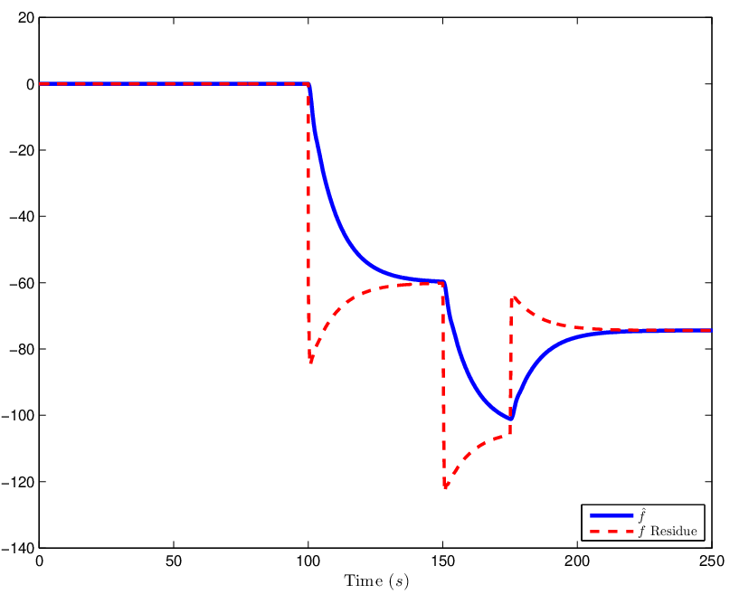
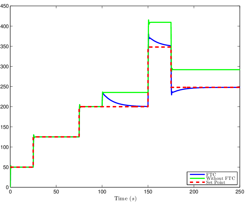
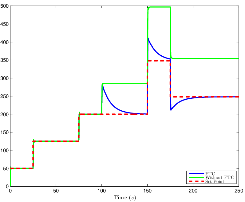
The test of open-loop scheme depicts the rewarding results in designing the mathematical ideas approaching the true system, constituting slightly just over $1\%$ error in average as illustrated in Table. II. The closed-loop scenario in Fig. (6(a)) also indicates the tracking to the set-point with slight overshoot while some rising set-point comes. This implies that the gain of the controller suit the system. Furthermore, the sensing element is supposed to be failure to draw the true system with two divergent outline related to sensitivity error, comprising $85\%$ and $70\%$ in certain iteration step. Those two patterns are simulated in Fig. (6(c)) and (6(d)) which conclude that in the $100^{th}-$ step the FTC could deal with the faulty states leading to trace the set-point whilst the system without FTC is unable to handle this situation and keeps performing the wrong tracking. The greater the faulty scenario will be, the greater the fault is created by the only-controller system. The ability of balancing the system constitutes FTC the method which is robust and preferable in industrial system if the faults on either sensor or actuator, even both, are occurred either in different time or simultaneously. Finally, Fig. (6(b)) infers the tracking from observer in terms of fault compared to the residual fault. The further research is to propose estimation methods to cope with unobservable system.

IV Conclusion

Mathematical designs of control system from, sensor, actuator, to scrubber have been proposed along with observer and fault-tolerant control. Closed-loop system indicates the rewarding performance to trace the set-point. The performance under FTC could deal with sensor fault in $100^{th}$ iteration. It could follow the set-point (blue) compared to that of without FTC (PI only) which keep demonstrating the faulty values with two different scenarios of faulty sensitivity. The created observer also emphasizes the rewarding results by the ability of fault estimation to cope with the $f$ residue. The following project is to place the faults on both actuator and sensor along with some variations of estimation methods apart from the conventional which could cope with the unobservability.

References

[1] A. D. Singh and S. Murugesan, “Fault-tolerant systems,” Computer, vol. 23, no. 7, pp. 15–17, July 1990.
[2] D. H. Zhou and P. M. Frank, “Fault diagnostics and fault tolerant control,” IEEE Transactions on Aerospace and Electronic Systems, vol. 34, no. 2, pp. 420–427, April 1998.
[3] J. Zhang and G. Yang, “Robust adaptive fault-tolerant control for a class of unknown nonlinear systems,” IEEE Transactions on Industrial Electronics, vol. 64, no. 1, pp. 585–594, Jan 2017.
[4] S. Song, J. Liu, and H. Wang, “Adaptive fault tolerant control for a class of nonlinear switched systems,” IEEE Access, vol. 6, pp. 7728–7738, 2018.
[5] M. Khalili, X. Zhang, Y. Cao, M. M. Polycarpou, and T. Parisini, “Distributed fault-tolerant control of multiagent systems: An adaptive learning approach,” IEEE Transactions on Neural Networks and Learning Systems, pp. 1–13, 2019.
[6] F. Boem, Y. Xu, C. Fischione, and T. Parisini, “Distributed fault detection using sensor networks and pareto estimation,” in 2013 European Control Conference (ECC), July 2013, pp. 932–937.
[7] M. K. Wafi, “Filtering module on satellite tracking,” AIP Conference Proceedings, vol. 2088, no. 1, p. 020045, 2019.
[8] K. Indriawati, N. Sebe, T. Agustinah, and A. Jazidie, “Robust fuzzy observer-based fault tolerant tracking control for nonlinear systems with simultaneous actuator and sensor faults: Application to a dc series motor speed drive,” International Review of Automatic Control (IREACO), vol. 8, no. 6, 2015.
[9] C. Zhang and I. M. Jaimoukha, “Fault-tolerant controller design with a tolerance measure for systems with actuator and sensor faults,” in 2017 American Control Conference (ACC), May 2017, pp. 4129–4134.
[10] T. H. Lee, C. P. Lim, S. Nahavandi, and R. G. Roberts, “Observer-based $\mathcal{H}_{\infty}$ fault-tolerant control for linear systems with sensor and actuator faults,” IEEE Systems Journal, vol. 13, no. 2, pp. 1981–1990, June 2019.
[11] X. Liu, Z. Gao, and A. Zhang, “Robust fault tolerant control for discrete-time dynamic systems with applications to aero engineering systems,” IEEE Access, vol. 6, pp. 18 832–18 847, 2018.
[12] Y. Zhang and J. Jiang, “Bibliographical review on reconfigurable fault-tolerant control systems,” Annual Reviews in Control, vol. 32, no. 2, pp. 229 – 252, 2008.
[13] T. A. Tran, “Research of the scrubber systems to clean marine diesel engine exhaust gases on ships,” Journal of Marine Science Research and Development, vol. 7, 11 2017.
[14] D. Kothari and P. Subbarao, Power Generation. Berlin, Heidelberg: Springer Berlin Heidelberg, 2009, pp. 1361–1419.
[15] K. Ogata, Modern Control Engineering, 4th ed. Upper Saddle River, NJ, USA: Prentice Hall PTR, 2001.
[16] M. Ichikawa, N. Sebe, K. Suyama, and K. Indriawati, “A bias fault estimation of actuators and sensors by optimization with $\ell_{0}$ -norm constraint,” in 2017 11th Asian Control Conference (ASCC), Dec 2017, pp. 1443–1448.