Reflected Diffusion Models

Aaron Lou Affiliation: Department of Computer Science, Stanford University Correspondence to: aaronlou@stanford.edu Stefano Ermon Affiliation: Department of Computer Science, Stanford University

Abstract

Score-based diffusion models learn to reverse a stochastic differential equation that maps data to noise. However, for complex tasks, numerical error can compound and result in highly unnatural samples. Previous work mitigates this drift with thresholding, which projects to the natural data domain (such as pixel space for images) after each diffusion step, but this leads to a mismatch between the training and generative processes. To incorporate data constraints in a principled manner, we present Reflected Diffusion Models, which instead reverse a reflected stochastic differential equation evolving on the support of the data. Our approach learns the perturbed score function through a generalized score matching loss and extends key components of standard diffusion models including diffusion guidance, likelihood-based training, and ODE sampling. We also bridge the theoretical gap with thresholding: such schemes are just discretizations of reflected SDEs. On standard image benchmarks, our method is competitive with or surpasses the state of the art without architectural modifications and, for classifier-free guidance, our approach enables fast exact sampling with ODEs and produces more faithful samples under high guidance weight.

Keywords:

Diffusion Models

Refer to caption — Figure 1: Overview of Reflected Diffusion Models. We map a data distribution $p_{0}$ supported on $\Omega$ to the prior distribution $p_{T}$ through a reflected stochastic differential equation (Section 3.1). Whenever a Brownian trajectory hits $\partial\Omega$ , it is reflected back in instead of escaping (circled in red), so $p_{t}$ is supported on $\Omega$ for all $t$ . We can recover $p_{0}$ from $p_{T}$ with a reversed reflected stochastic differential equation (Section 3.2) by learning the Stein score $\nabla_{x}\log p_{t}$ (Section 4). Our generative model is guaranteed to be constrained in $\Omega$ .

1 Introduction

Originally introduced in Sohl-Dickstein et al. 2015 and later augmented in Song & Ermon 2019b; Ho et al. 2020; Song et al. 2021b, diffusion models have quickly become one of the most ubiquitous deep generative models, with applications in many domains including images (Dhariwal & Nichol 2021), natural language (Li et al. 2022), and molecule generation (Xu et al. 2022). Additionally, their stability and scabality have enabled the deployment of large text-to-image systems (Ramesh et al. 2022).^†^† Code Link: https://github.com/louaaron/Reflected-Diffusion/

Diffusion models learn to reverse a stochastic process that maps data to noise, but, as a result of inherent approximation error of both the SDE discretization and score matching, they often follow incorrect trajectories. This behavior compounds error, so models can diverge and generate highly unnatural samples on more complex tasks (see for instance Figure 3). To mitigate this degeneration, many diffusion models modify the sampling process by projecting to the support of the data after each diffusion step (Ho et al. 2020; Li et al. 2022), a technique known as thresholding. This incorporates the known constraints of the data distribution, stabilizing sampling and avoiding divergent behavior. Notably, this oft-overlooked detail underlies many pixel-based image diffusion models (Ho et al. 2020; Dhariwal & Nichol 2021) (appearing as a $[0,255]$ clipping function at each diffusion step) and is essential for text-to-image generation (Saharia et al. 2022). Although thresholding avoids failure, it is theoretically unprincipled because it leads to a mismatch between the training and generative processes. Furthermore, this mismatch can introduce artifacts such as oversaturation (Ho & Salimans 2022) that necessitate further modifications (Saharia et al. 2022).

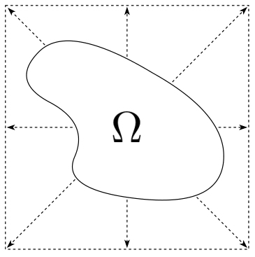
In this work, we present Reflected Diffusion Models, a class of diffusion models that, by design, respects the known support of the data distribution. Unlike standard diffusion models, which perturbs the data density with Brownian motion, our method evolves the distribution with reflected Brownian motion that always stays within the boundary. We then parameterize the reversed diffusion process with the scores of the perturbed density, which we learn using a new score matching method on bounded domains. The resulting generative model is a reflected SDE that automatically incorporates the data constraints without altering the generative process. We provide an overview of our method in Figure 1.

Our proposed methodology has several merits:

Scales to high dimensions. To learn the score function on a general bounded domain, we introduce constrained denoising score matching (CDSM). Unlike previous methods (Hyvärinen 2007), CDSM scales to high dimensions, and we develop an algorithm for fast computation. Since reflection operations are negligible compared to neural network computation, our training and inference times are effectively equivalent to those of standard diffusion models.

Key features transfer over. We show that ODE sampling (Song et al. 2021b), diffusion guidance (Ho & Salimans 2022), and maximum likelihood bounds (Song et al. 2021a) extend to the reflected setting. As such, our method can be modularly applied to preexisting diffusion model systems.

Justifying and correcting previous methods. We draw connections with the thresholding methods used in pixel-space diffusion models (Saharia et al. 2022). These methods all sample from a reflected stochastic differential equation despite being trained on a standard diffusion process. Correctly training with our CDSM loss avoids pathological behavior and allows for equivalent ODE sampling.

Broad Applicability. We apply our method to high-dimensional simplices (e.g. class probabilities) and hypercubes (e.g. images). Using a synthetic example, we show that our method is the a simplex diffusion model that scales to high dimensions. On common image generation benchmarks, our results are competitive with or surpass the current state of the art. In particular, on unconditional CIFAR-10 generation (Krizhevsky 2009), we achieve a state of the art Inception Score of 10.46 and a comparable FID score of 2.72. For likelihood estimation, our method achieves a second best score of 2.68 and 3.74 bits per dimension on CIFAR-10 and ImageNet32 (van den Oord et al. 2016) without relying on either importance sampling or learned noise schedules.

2 Background

To introduce diffusion models (in the continuous time formalism of (Song et al. 2021b)), we first transform a data density $q_{0}$ on $\mathbb{R}^{d}$ by applying a “forward” diffusion process. This takes the form of perturbing points $\mathbf{x}_{0}\sim q_{0}$ with an SDE with a fixed drift coefficient $\mathbf{f}:\mathbb{R}^{d}\times\mathbb{R}\to\mathbb{R}^{d}$ , diffusion coefficient $g:\mathbb{R}\to\mathbb{R}$ , and Brownian motion $\mathbf{B}_{t}$ :

\mathrm{d}\mathbf{x}_{t}=\mathbf{f}(\mathbf{x}_{t},t)\mathrm{d}t+g(t)\mathrm{d}\mathbf{B}_{t}

(1)

The resulting family of time varied distributions $x_{t}\sim q_{t}$ approaches a known prior distribution $q_{T}\approx\mathcal{N}(0,\sigma_{T}^{2}I)$ . This density evolution process can be reversed by perturbing samples $x_{T}\sim q_{T}$ with a reversed SDE (Anderson 1982):

\mathrm{d}\mathbf{x}_{t}=(\mathbf{f}(\mathbf{x}_{t},t)-g^{2}(t)\nabla_{x}\log q_{t}(\mathbf{x}_{t}))\mathrm{d}t+g(t)\mathrm{d}\overline{\mathbf{B}}_{t}

(2)

where $\overline{\mathbf{B}}_{t}$ is time reversed Brownian motion. Diffusion models approximate this reverse process by learning $\nabla_{x}\log q_{t}$ , known as the score function, through a $\lambda$ -weighted score matching loss:

\mathbb{E}_{t,\mathbf{x}_{t}\sim q_{t}}\lambda_{t}\left\|\mathbf{s}_{\theta}(\mathbf{x}_{t},t)-\nabla_{x}\log q_{t}(\mathbf{x}_{t})\right\|^{2}

(3)

which most commonly takes the form of the more tractable denoising score matching loss (Vincent 2011):

\hskip-4.97922pt\mathbb{E}_{t,\mathbf{x}_{0}\sim q_{0},\mathbf{x}_{t}\sim q_{t}(\cdot|\mathbf{x}_{0})}\lambda_{t}\left\|\mathbf{s}_{\theta}(\mathbf{x}_{t},t)-\nabla_{x}\log q_{t}(\mathbf{x}_{t}|\mathbf{x}_{0})\right\|^{2}

(4)

Here, $q_{t}(\mathbf{x}_{t}|\mathbf{x}_{0})$ is the transition kernel induced by the SDE in Equation 1. With a learned score $\mathbf{s}_{\theta}(\mathbf{x},t)\approx\nabla_{x}\log q_{t}$ , one can define a generative model by first sampling $\mathbf{y}_{T}\sim\mathcal{N}(0,\sigma_{T}^{2}I)$ and then solving the reverse SDE

\mathrm{d}\mathbf{y}_{t}=(\mathbf{f}(\mathbf{y}_{t},t)-g(t)^{2}\mathbf{s}_{\theta}(\mathbf{y}_{t},t))\mathrm{d}t+g(t)\mathrm{d}\overline{\mathbf{B}}_{t}

(5)

from time $T$ to $0$ , giving an approximate sample from $q_{0}$ .

Diffusion models enjoy many special properties. For example, for certain $\lambda_{t}$ , Equation 4 can be reformulated as an ELBO using Girsanov’s theorem (Song et al. 2021a; Kingma et al. 2021; Huang et al. 2021), allowing for maximum likelihood training. Furthermore, one can derive an equivalent Neural ODE that can be used for sampling and exact likelihood evaluation (Chen et al. 2018).

Guidance. One can also control the diffusion model to sample from a synthetic distribution $\tilde{q}_{t}(\mathbf{x}_{t}|c)\propto q_{t}(c|\mathbf{x_{t}})^{w}q_{t}(\mathbf{x}_{t})$ . Here, $c$ is a desired condition such as a class or text description, and interpolating the guidance weight $w$ controls the fidelity and diversity of the samples. This requires the score

\begin{gathered}\nabla_{x}\log\tilde{q}_{t}(\mathbf{x}_{t}|c)=w\nabla_{x}\log q_{t}(c|\mathbf{x}_{t})+\nabla_{x}\log q_{t}(\mathbf{x}_{t})\end{gathered}

(6)

which can be learned $\tilde{\mathbf{s}}_{\theta}(\mathbf{x}_{t},t,c)\approx\nabla_{x}\log\tilde{q}_{t}(\mathbf{x}_{t}|c)$ without requiring explicit training on $\tilde{q}_{t}$ . For example, classifier guided methods (Song et al. 2021b; Dhariwal & Nichol 2021) combine a pretrained score function $\mathbf{s}_{\theta}(\mathbf{x}_{t},t)$ and classifier $q_{t}(c|\mathbf{x}_{t})$ :

\tilde{\mathbf{s}}_{\theta}(\mathbf{x}_{t},t,c):=w\nabla_{x}\log q_{t}(c|\mathbf{x}_{t})+\mathbf{s}_{\theta}(\mathbf{x}_{t},t)

(7)

and classifier-free guidance methods (Ho & Salimans 2022) uses a $c$ -conditioned score function and an implicit Bayes classifier $q_{t}(c|\mathbf{x}_{t})=\frac{q_{t}(\mathbf{x}_{t}|c)}{q_{t}(\mathbf{x}_{t})q_{t}(c)}$

\tilde{\mathbf{s}}_{\theta}(\mathbf{x}_{t},t,c):=(w+1)\mathbf{s}_{\theta}(\mathbf{x}_{t},t,c)-w\mathbf{s}_{\theta}(\mathbf{x}_{t},t)

(8)

Thresholding. However, since $\mathbf{s}_{\theta}$ is not a perfect score function, there is a mismatch between the modeled backward process and the true forward process. Thus, diffusion models can push a sample to areas where $q_{t}(\mathbf{x}_{t})$ is small, which creates a negative feedback loop since score matching struggles in low probability areas (Song & Ermon 2019a; Koehler et al. 2022). This causes the sampling process to diverge and commonly occurs for more complex tasks, especially those involving diffusion guidance.

To combat this, many previous works alter the diffusion sampling procedure using thresholding (Saharia et al. 2022; Li et al. 2022), which stabilizes the sampling process with inductive biases from the data. In particular, thresholding applies an operator $\mathcal{O}$ that projects back to the data domain $\Omega$ during each discretized SDE step:

\mathbf{y}_{t-\Delta t}=\mathcal{O}(\mathbf{y}_{t}-\left[\mathbf{f}(\overline{\mathbf{y}}_{t},t)-g(t)^{2}\mathbf{s}_{\theta}(\mathbf{y}_{t},t)\right]\Delta t)+g(t)\mathbf{B}_{\Delta t}

(9)

For the case of images, $\mathcal{O}$ can be static thresholding, which clips each dimension to the pixel range $[0,255]$ , and dynamic thresholding, which first normalizes all pixels by the $p$ -th percentile pixel before clipping (Saharia et al. 2022).

Thresholding alleviates divergent sampling but comes with considerable downsides. For example, it breaks the theoretical setup since the generative model no longer approximates the reverse diffusion process. This mismatch induces artifacts during sampling and precludes the use of ODE sampling (Song et al. 2021b).

3 Reflected Diffusion Models

In this section, we present Reflected Diffusion Models. These define a generative model on a data domain $\Omega$ (assumed to be connected and compact with nonempty interior and uniform Hausdorff dimension) which outer-bounds the support of the data distribution $p_{0}$ . Our method retains the theoretical underpinnings of diffusion models while incorporating inductive biases from thresholding. We highlight the core mechanisms in Figure 1.

3.1 Reflected Stochastic Differential Equations

To model diffusion processes on a compact domain $\Omega$ , we use reflected SDEs. For ease of presentation, we only give an intuitive definition of reflected SDEs and simplify so that $g$ is scalar and $\mathbf{L}_{t}$ reflects in the normal direction. In Appendix A.1, we provide a more rigorous mathematical definition and generalize to matrix diffusion coefficients and oblique reflections. For a full introduction, we recommend the readers consult a monograph such as Pilipenko 2014.

Our reflected SDEs perturb an initial datum $\mathbf{x}_{0}\sim p_{0}$ and are parameterized by a drift coefficient $\mathbf{f}:\Omega\times\mathbb{R}\to\mathbb{R}^{d}$ and diffusion coefficient $g:\mathbb{R}\to\mathbb{R}$ :

\mathrm{d}\mathbf{x}_{t}=\mathbf{f}(\mathbf{x}_{t},t)\mathrm{d}t+g(t)\mathrm{d}\mathbf{B}_{t}+\mathrm{d}\mathbf{L}_{t}

(10)

The first two terms on the right hand side of Equation 10 are exactly those of Equation 1, showing that our reflected SDE behaves like a regular SDE in the interior of $\Omega$ . $\mathbf{L}_{t}$ is the additional boundary constraint that, intuitively, forces the particle to stay inside $\Omega$ . When $x_{t}$ hits $\partial\Omega$ , $\mathbf{L}_{t}$ neutralizes the outward normal-pointing component.

This reflected SDE has a unique strong solution as long as $\mathbf{f}$ and $g$ are Lipschitz in state and time and $\Omega$ satisfies the uniform exterior sphere condition (Pilipenko 2014, Theorem 2.5.4), which ensures that $\partial\Omega$ is sufficiently regular. In particular, the uniform exterior sphere condition holds true when $\partial\Omega$ is smooth and even when $\Omega$ is a convex polytope.

3.2 Density Evolution and Time Reversal

When we perturb $p_{0}$ with the reflected SDE in Equation 10, our density evolves according to the Fokker-Planck equation with Neumann boundary condition (Schuss 2013):

\begin{gathered}\frac{\partial}{\partial t}p_{t}=\ddiv(-p_{t}\mathbf{f}+\frac{g^{2}}{2}\nabla_{x}p_{t})\\ (p_{t}\mathbf{f}-\frac{g^{2}}{2}\nabla_{x}p_{t})\cdot\mathbf{n}=0,\mathbf{x}\in\partial\Omega,\mathbf{n}\text{ normal},t>0\end{gathered}\vskip-2.84526pt

(11)

In addition to allowing us to characterize the limiting density $p_{T}$ , this induces a reversed reflected stochastic differential equation (Cattiaux 1988; Williams 1988):

\begin{gathered}\mathrm{d}\mathbf{x}_{t}=(\mathbf{f}(\mathbf{x}_{t},t)-g(t)^{2}\nabla_{x}\log p_{t}(\mathbf{x}_{t}))\mathrm{d}t\\ +g(t)\mathrm{d}\overline{\mathbf{B}}_{t}+\mathrm{d}\overline{\mathbf{L}}_{t}\end{gathered}

(12)

where $\overline{\mathbf{L}}_{t}$ is the reversed boundary condition. For our case, $\overline{\mathbf{L}}_{t}$ also reflects in the normal direction.

Remark 3.1.

The reversed reflected SDE closely resembles the reversed standard SDE given in Equation 2. On one hand, this is natural because local dynamics match: when $\Omega=\mathbb{R}^{d}$ , $\mathbf{L}_{t}$ disappears since $\mathbf{x}_{t}$ can never hit $\partial\mathbb{R}^{d}=\emptyset$ . On the other hand, it is surprising that we can reverse a reflected diffusion process with another reflected diffusion process, something that does not hold in the discrete time case.

3.3 Reflected SDEs in Practice

In our experiments, $\Omega$ will be either the unit cube $C_{d}:=\{\mathbf{x}\in\mathbb{R}^{d}:0\leq x_{i}\leq 1\}$ or the unit simplex, which is given by $\Delta_{d}:=\{\mathbf{x}\in\mathbb{R}^{d}:\sum_{i=1}^{d}x_{i}=1,x_{i}\geq 0\}$ . We often find it more convenient to work with the projected simplex $\overline{\Delta}_{d}:=\{\mathbf{x}\in\mathbb{R}^{d}:\sum_{i=1}^{d-1}x_{i}\leq 1,x_{i}\geq 0\}$ as it is bounded in $\mathbb{R}^{d}$ instead of in a hyperplane.

We will diffuse with the Reflected Variance Exploding SDE (RVE SDE), a generalization of the Variance-Exploding SDE introduced in Song et al. 2021b. A RVE SDE is parameterized by $\sigma_{0}\ll\sigma_{1}$ and is defined for $t\in[0,1]$ by

\mathrm{d}\mathbf{x}_{t}=\overline{\sigma}_{t}\mathrm{d}\mathbf{B}_{t}+\mathrm{d}\mathbf{L}_{t}

(13)

where $\overline{\sigma}_{t}:=\sigma_{0}^{1-t}\sigma_{1}^{t}\sqrt{2\log\left(\frac{\sigma_{1}}{\sigma_{0}}\right)}$ . The reverse is

\mathrm{d}\mathbf{x}_{t}=-\overline{\sigma}_{t}^{2}\nabla_{x}\log p_{t}(\mathbf{x}_{t})\mathrm{d}t+\overline{\sigma}_{t}\mathrm{d}\overline{\mathbf{B}}_{t}+\mathrm{d}\overline{\mathbf{L}}_{t}

(14)

Note that the RVE SDE corresponds to a time dilated version of reflected Brownian motion: time $t$ of a RVE SDE corresponds to time $\sigma_{t}$ of reflected Brownian motion, where $\sigma_{t}:=\sigma_{0}^{1-t}\sigma_{1}^{t}$ . As a result of Equation 11, $p_{0}$ evolves under a heat equation with Neumann boundary conditions:

\begin{gathered}\frac{\partial}{\partial t}p_{t}=\frac{g(t)^{2}}{2}\Delta_{x}p_{t}\quad\nabla_{x}p_{t}\cdot\mathbf{n}=0\text{ on }\partial\Omega\end{gathered}

(15)

Note that $p_{1}$ becomes a uniform density over $\Omega$ for large enough $\sigma_{1}$ . To see this, we can draw intuition from physics: heat homogenizes in a closed container.

4 Score Matching on Bounded Domains

While the reflected SDE framework provides a nice theoretical pathway to construct a reflected diffusion model, it requires one to learn the score function $\mathbf{s}_{\theta}\approx\nabla_{x}\log p_{t}$ on $\Omega$ . We minimize the constrained score matching loss:

\frac{1}{2}\mathbb{E}_{\mathbf{x}\sim p}^{\Omega}\left\|\mathbf{s}_{\theta}(\mathbf{x})-\nabla_{x}\log p(\mathbf{x})\right\|^{2}

(16)

where we omit time-dependence for presentation purposes. Furthermore, $\mathbb{E}^{\Omega}$ indicates the domain of the expectation (as opposed to $\mathbb{E}$ which is an integral over $\mathbb{R}^{d}$ ). This is because $p$ can be discontinuous at $\partial\Omega$ (since it is $0$ outside of $\Omega$ and can be nonzero on $\partial\Omega$ ), so constraining the integral ensure regularity properties used for theorems (such as Stokes’).

In this section, we review previous methods for score matching on bounded domains, discuss their fundamental limitations, and propose constrained denoising score matching to overcome these difficulties. Additionally, for the RVE SDE introduced in Section 3.3, we show how to quickly compute the score matching training objective.

4.1 Pitfalls of Implicit Score Matching

One may hope to draw inspiration from the standard paradigm, which transforms the score matching integral

\frac{1}{2}\mathbb{E}_{\mathbf{x}\sim q}\left\|\mathbf{s}_{\theta}(\mathbf{x})-\nabla_{x}\log q(\mathbf{x})\right\|^{2}

(17)

into the implicit score matching loss (Hyvärinen 2005):

\mathbb{E}_{\mathbf{x}\sim q}\left[\ddiv(\mathbf{s}_{\theta})(\mathbf{x})+\frac{1}{2}\left\|\mathbf{s}_{\theta}(\mathbf{x})\right\|^{2}\right]

(18)

This removes the intractable $\nabla_{x}\log q(\mathbf{x})$ , allowing for estimation using Monte Carlo sampling. However, the derivation requires the use of Stokes’ theorem; applying Stokes’ theorem to Equation 16 would instead result in

\begin{gathered}\mathbb{E}_{\mathbf{x}\sim p}^{\Omega}\left[\ddiv(\mathbf{s}_{\theta})(\mathbf{x})+\frac{1}{2}\left\|s_{\theta}(\mathbf{x})\right\|^{2}\right]\\ +\int_{\partial\Omega}p(\mathbf{x})\left\langle\mathbf{s}_{\theta}(\mathbf{x}),\mathbf{n}(\mathbf{x})\right\rangle\mathrm{d}\mathbf{x}\end{gathered}

(19)

where $\mathbf{n}(\mathbf{x})$ is the interior pointing normal vector. Unlike the case of $\Omega=\mathbb{R}^{d}$ , where the second term disappears since $\partial\mathbb{R}^{d}=\emptyset$ , this result is computationally intractable. Thus, previous work instead proposes to re-weight the loss function with a nonnegative function $h$ that vanishes on the boundary (Hyvärinen 2007; Yu et al. 2020), minimizing

\frac{1}{2}\mathbb{E}_{\mathbf{x}\sim p}^{\Omega}h(\mathbf{x})\left\|\mathbf{s}_{\theta}(\mathbf{x})-\nabla_{x}\log p(\mathbf{x})\right\|^{2}

(20)

Since $h$ vanishes on $\partial\Omega$ , we can cleanly apply Stokes’ theorem and derive a result without a boundary term, giving an implicit score matching loss:

\mathbb{E}_{\mathbf{x}\sim p}^{\Omega}\left[\ddiv(h\cdot\mathbf{s}_{\theta})(\mathbf{x})+\frac{h(\mathbf{x})}{2}\left\|\mathbf{s}_{\theta}(\mathbf{x})\right\|^{2}\right]

(21)

However, this formulation is not suitable for high dimensions, even with fast numerical algorithms for the divergence operator (Hutchinson 1989; Song et al. 2019). This is because the loss is downweighted near the boundaries, so, for a fixed budget, the error can become unbounded as $x\to\partial\Omega$ . For high dimensions, the space near the boundary becomes an increasingly larger proportion of the total volume¹¹ 1 Consider the case when $\Omega=[0,1]^{d}$ . For large $d$ , almost all the mass is close to the boundary., which greatly hampers the sample efficiency of the loss.

4.2 Constrained Denoising Score Matching

Inspired by the empirical success of denoising score matching (Vincent 2011; Song & Ermon 2019a), we present constrained denoising score matching (CDSM). Crucially, denoising score matching, unlike implicit score matching, can directly generalize to bounded domains due to how it handles discontinuities. This means that, unlike previous methods for constrained score matching, the derivation transfers smoothly. The core mechanism is presented in the following proposition, which we prove in Appendix A.2.

Proposition 4.1.

Suppose that we perturb an $\Omega$ -supported density $a(\mathbf{x})$ with noise $b(\mathbf{x}|\cdot)$ (also supported on $\Omega$ ) to get a new density $b(\mathbf{x}):=\int_{\Omega}a(\mathbf{y})b(\mathbf{x}|\mathbf{y})\mathrm{d}\mathbf{y}$ . Then, under suitable regularity conditions for the smoothness of $a$ and $b$ , the score matching loss for $b$ :

\frac{1}{2}\mathbb{E}_{\mathbf{x}\sim b}^{\Omega}\left\|\mathbf{s}_{\theta}(\mathbf{x})-\nabla_{x}\log b(\mathbf{x})\right\|^{2}

(22)

is equal (up to a constant factor that does not depend on $\mathbf{s}$ ) to the CSDM loss:

\frac{1}{2}\mathbb{E}_{\mathbf{x}_{0}\sim a}^{\Omega}\mathbb{E}_{\mathbf{x}\sim b(\cdot|\mathbf{x}_{0})}^{\Omega}\left\|\mathbf{s}_{\theta}(\mathbf{x})-\nabla_{x}\log b(\mathbf{x}|\mathbf{x}_{0})\right\|^{2}

(23)

With the constrained denoising score matching loss, we are then able to define a training objective for reflected diffusion models. In particular, since $p_{t}(\mathbf{x})$ is a by definition perturbed density of $p_{0}(\mathbf{x})$ with transition kernel $p_{t}(\mathbf{x}|\cdot)$ , the weighted score score matching loss directly becomes:

\mathbb{E}_{t,\mathbf{x}_{0}\sim p_{0},\mathbf{x}_{t}\sim p_{t}(\cdot|\mathbf{x}_{0})}^{\Omega}\lambda_{t}\left\|\mathbf{s}_{\theta}(\mathbf{x}_{t},t)-\nabla_{x}\log p_{t}(\mathbf{x}_{t}|\mathbf{x}_{0})\right\|^{2}

(24)

For our reflected SDE, we will set $\lambda_{t}\propto g(t)^{2}$ , mirroring previous work and minimizing variance during optimization. Interestingly, as we prove in Section 7, this corresponds to an ELBO loss when we reverse a RVE SDE.

4.3 Scaling Score Matching Computation

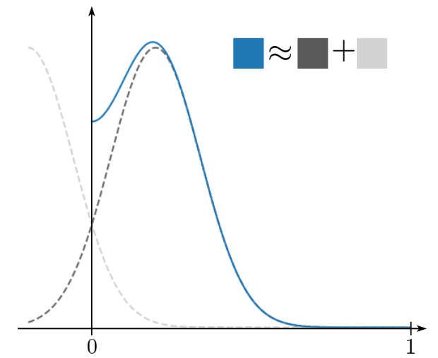
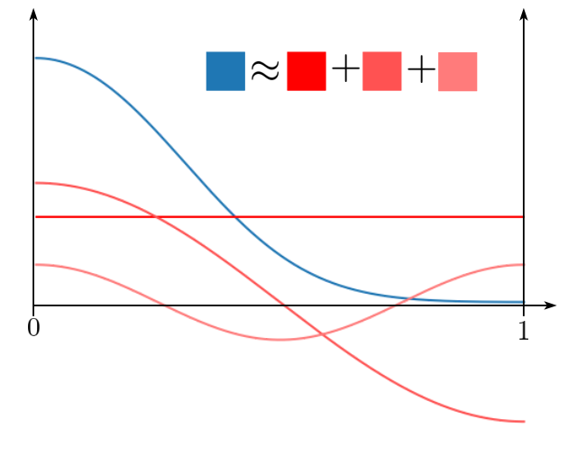
We finalize by showing how to sample from and compute the score of the transition density $p_{t}(\mathbf{x}_{t}|\mathbf{x}_{0})$ for the RVESDE. Note that this is the transition density of a reflected Brownian Motion (Harrison & Reiman 1981). We highlight the key features of our method in Figure 2.

Sampling. To sample from $p_{t}(\mathbf{x}_{t}|\mathbf{x}_{0})$ , we can repeatedly reflect a sample $\mathbf{y}$ from $\mathcal{N}(\mathbf{x}_{0},\frac{\sigma_{t}^{2}}{2}I)$ . In particular, we follow the line segment $t\to t\mathbf{y}+(1-t)\mathbf{x}_{0}$ , reflecting in the normal direction when it crosses $\partial\Omega$ and repeating until we reach $t=1$ . This works because, intuitively, the boundary redirects the the Brownian motion but does not change the magnitude. In practice, this process can be quickly computed with classic computational geometric techniques.

Score Computation. There are two approaches for computing the score of $p_{t}(\mathbf{x}_{t}|\mathbf{x}_{0})$ on general geometric domains:

Approximation with Sum of Gaussians (Jing et al. 2022b). This method decomposes $p_{t}(\mathbf{x}_{t}|\mathbf{x}_{0})$ into an infinite sum of Gaussian densities that depend on $\mathbf{x}_{0}$ , $\mathbf{x}_{t}$ , and the geometry of the domain. For our bounded $\Omega$ with the reflection condition, this gives us the equation

p_{t}(\mathbf{x}_{t}|\mathbf{x}_{0})=\sum_{\mathbf{x}^{\prime}\in\mathcal{R}(\mathbf{x}_{t})}p_{\mathcal{N}\left(\mathbf{x}_{0},\sigma_{t}^{2}/2\cdot I\right)}(\mathbf{x}^{\prime})

(25)

where $p_{\mathcal{N}\left(\mathbf{x}_{0},\sigma_{t}^{2}/2\cdot I\right)}$ is the pdf of the Gaussian centered at $\mathbf{x}_{0}$ with variance $\sigma_{t}^{2}I$ and $\mathcal{R}(\mathbf{x}_{t})$ is the set of all $\mathbf{x}^{\prime}\in\mathbb{R}^{d}$ s.t. the repeated reflection of the path $t\to t\mathbf{x}^{\prime}+(1-t)\mathbf{x}_{0}$ ends in $\mathbf{x}_{t}$ . Note that this reflection scheme is the same one we use for sampling. Furthermore, through elementary derivations, this gives us a formula for the score $\nabla_{x}\log p_{t}(\mathbf{x}_{t}|\mathbf{x_{0}})$ .

Generally, this method works quite well for small $\sigma_{t}$ , as we only need to take a small number of local reflections to approximate $p_{t}(\mathbf{x}_{t}|\mathbf{x}_{0})$ . However, for larger $\sigma_{t}$ , we need to take many more reflections since the underlying Gaussian is too dispersed, greatly increasing the computational cost.

Approximation with Laplacian Eigenfunctions (Bortoli et al. 2022). This method instead computes using Laplacian Eigenfunctions, a standard technique for solving the heat equation (Evans 2010). For our problem, these are a (known for each $\Omega$ ) set of functions $f_{i}\in L^{2}(\Omega),i\in\mathbb{N}$ that satisfy $\Delta f_{i}=-\lambda_{i}f_{i}$ and $\nabla f_{i}\cdot\mathbf{n}=0$ on $\partial\Omega$ . In particular, these form an orthonormal basis for $L^{2}(\Omega)$ , allowing us to solve Equation 15 directly for an initial density of $\delta_{\mathbf{x}_{0}}$ :

p_{t}(\mathbf{x}_{t}|\mathbf{x}_{0})=\sum_{i=0}^{\infty}e^{-\lambda_{i}\sigma_{t}^{2}/2}f_{i}(\mathbf{x}_{t})f_{i}(\mathbf{x}_{0})

(26)

This method works well for large $\sigma_{t}$ because this means that $e^{-\lambda_{i}\sigma_{t}^{2}/2}\to 0$ , removing the need to evaluate many of the terms. However, for small $\sigma_{t}$ , this method becomes costly because it requires many more terms. Similar to the above method, we can derive a formula for $\nabla_{x}\log p_{t}(\mathbf{x}_{t}|\mathbf{x_{0}})$ through this sum.

Our Method. We instead propose to combine the above two approaches. In particular, we note that they complement each other: Gaussian sum is accurate for small $\sigma_{t}$ and eigenfunction sum is accurate for large $\sigma_{t}$ . We can therefore set a $\sigma^{\prime}\in(\sigma_{0},\sigma_{1})$ and compute with Gaussian sum when $\sigma_{t}<\sigma^{\prime}$ and with eigenfunction sum when $\sigma_{t}>\sigma^{\prime}$ . In practice, this allows us to upper-bound the number of reflections/eigenfunctions used to $\approx 5$ , much fewer than the exponential amount required for each method individually.

Scaling to High Dimensions. By itself, this branching method is unfortunately not enough to scale to very high dimensions. In particular, our computation is, in the worst case, $O(d^{k})$ where $d$ is the dimension of $\Omega$ and $k$ is the number of reflection steps or the highest eigenfunction frequency. We have only bounded $k$ to something more manageable.

To overcome this scaling issue, we consider the simple case of the hypercube $[0,1]^{d}$ . Since our Brownian motion does not have inter-dimensional interactions, reflections do not interact between non-parallel hyperplanes, and Laplacian eigenfunctions factorize by dimension, we can decompose the probability along each component interval:

p_{t}(\mathbf{x}_{t}|\mathbf{x}_{0})=\prod_{i=1}^{d}p_{t}^{i}(x_{t}^{i}|x_{0}^{i})

(27)

where $x_{t}^{i}$ and $x_{0}^{i}$ are the $i$ -components of $\mathbf{x}_{t}$ and $\mathbf{x}_{0}$ respectively and $p_{t}^{i}$ is the marginal probability on the $i$ -th coordinate. Note that the RVE SDE on $[0,1]^{d}$ marginalizes to a RVE SDE on $[0,1]$ for each dimension:

\mathrm{d}x_{t}^{i}=\overline{\sigma}_{t}\mathrm{d}B_{t}^{i}+\mathrm{d}L_{t}^{i}

(28)

where $B_{t}^{i}$ and $L_{t}^{i}$ are the Brownian motion and boundary condition (respectively) for dimension $i$ . We can therefore compute on each $\Omega_{i}=[0,1]$ and combine the results, reducing the cost from $O(d^{k})$ to $O(kd)$ . Regular score matching is $O(d)$ , and since $k$ is small, we can train Reflected Diffusion Models just as quickly as regular diffusion models.

For more general domains, under certain conditions, we can smoothly and bijectively map from $\mathrm{int}(\Omega)\to(0,1)^{d}$ . Thus, we can instead learn a diffusion model on $[0,1]^{d}$ and then project back to $\Omega$ . More details are given in Appendix B.2. In particular, this mapping procedure allows us to learn a diffusion model on high-dimensional simplices $\Delta_{d}$ .

5 Simulating Reflected SDEs

Combining a score $\mathbf{s}_{\theta}$ learned through CSDM and the reverse reflected SDE, we have a Reflected Diffusion Model: sample $\mathbf{x}_{T}\sim\mathcal{U}(\Omega)$ and solve the reflected SDE:

\mathrm{d}\mathbf{x}_{t}=-\overline{\sigma}_{t}^{2}\mathbf{s}_{\theta}(\mathbf{x}_{t},t)\mathrm{d}t+\overline{\sigma}_{t}\mathrm{d}\overline{\mathbf{B}}_{t}+\mathrm{d}\overline{\mathbf{L}}_{t}

(29)

In this section, we examine numerical methods for simulating examples from this reflected SDE.

5.1 Euler-Maruyama Discretizations and Thresholding

The typical Euler-Maruyama discretization of a standard SDE (Equation 1) is given by

\mathbf{x}_{t+\Delta t}=\mathbf{x}_{t}+\mathbf{f}(\mathbf{x}_{t},t)\Delta t+g(t)\mathbf{B}_{\Delta t}

(30)

where $\mathbf{B}_{\Delta t}\sim\mathcal{N}(0,\Delta t\cdot I)$ . For reflected SDEs, one can adapt this discretization by approximating the effect of $\mathbf{L}_{t}$ with some suitable operators $\mathcal{O}$ .

\mathbf{x}_{t+\Delta t}=\mathcal{O}(\mathbf{x}_{t}+\mathbf{f}(\mathbf{x}_{t},t)\Delta t+g(t)\mathbf{B}_{\Delta t})

(31)

Common examples of $\mathcal{O}$ include the projection operator $\proj(x)=\argmin_{y\in\Omega}d(x,y)$ (Liu 1993) or the reflection operator $\refl$ used in Section 4.3 (Schuss 2013). One can see that, as $\Delta t\to 0$ , both the projection and reflection schemes converge in distribution. Empirically, we find that reflection generates better samples.

Interestingly, this closely mirrors the thresholding step given in Equation 9, with the only difference being the choice of operator $\mathcal{O}$ and whether $\mathcal{O}$ is applied before or after the noise step. This difference disappears when $\Delta t\to 0$ :

Proposition 5.1 (Thresholding solves a reflected SDE).

Both types of thresholding solve the reflected SDE (Equation 10) as $\Delta t\to 0$ under suitable conditions.

The full proposition and proof are given in Appendix A.5.

5.2 Predictor Corrector

We extend the predictor-corrector (PC) framework of Song et al. 2021b, which has been shown to improve results. In particular, our learned scores can be used to augment the sampling procedure using Langevin Dynamics (Song & Ermon 2019a). However, this requires Langevin dynamics for a constrained domain (Bubeck et al. 2015), which, for the probability $p$ , are given by the reflected SDE:

\mathrm{d}\mathbf{x}_{t}=\frac{1}{2}\nabla_{x}\log p(\mathbf{x}_{t})\mathrm{d}t+\mathrm{d}\mathbf{B}_{t}+\mathrm{d}\mathbf{L}_{t}

(32)

During our reversed diffusion iterations, we can discretize the langevin dynamics using Reflected Euler-Maruyama and apply our learned score $\mathbf{s}(\cdot,t)$ :

\mathbf{x}_{t}^{\prime}=\refl(\mathbf{x}_{t}+\frac{\epsilon}{2}\mathbf{s}_{\theta}(\mathbf{x}_{t},t)+\sqrt{2\epsilon}\cdot\mathbf{z})\quad\mathbf{z}\sim\mathcal{N}(0,1)

(33)

In practice, we find that PC sampling with a small signal-to-noise ratio noticeably improves image generation results.

CIFAR-10 Quality Results. With these components, we test our method for image generation on the CIFAR-10 dataset and report Inception Score (IS) (Salimans et al. 2016) and Frechet Inception Distance (FID) (Heusel et al. 2017) in table 1. Our models remain competitive, achieving a SOTA Inception score of 10.42. However, Tweedies’ formula does generalize to reflected diffusion (Efron 2011) (more details are in Appendix B.3), so our model generates images with imperceptible noise (on the scale of $1-2$ pixels), which degrades the FID score to 2.72 (Jolicoeur-Martineau et al. 2020). Despite this, our samples are diverse and visually indistinguishable (Appendix D).

Model	IS $\uparrow$	FID $\downarrow$
NCSN++ (Song et al. 2021b)	9.89	2.20
DDPM++ (Song et al. 2021b)	9.68	2.41
Styleformer (Park & Kim 2021)	9.94	2.82
UNCSN++ (Kim et al. 2021)	10.11	–
VitGAN (Lee et al. 2021)	9.89	4.87
Subspace NCSN++ (Jing et al. 2022a)	9.99	2.17
EDM (Karras et al. 2022)	–	1.97
Reflected Diffusion (ours)	10.46	2.72

Table 1: CIFAR10-Sample Quality Results. We test Reflected Diffusion Models on CIFAR-10 Image Generation and report IS and FID scores. Our model is highly competitive, achieving a state of the art-inception score for unconditional generation. However, FID lags behind due to noise (as discussed in Appendix B.3)

5.3 Probability Flow ODE

Similarly to the probability flow ODE derived in Song et al. 2021b, one can construct an equivalent deterministic process for a reflected SDE. Interestingly, doing this removes the boundary reflection term, so our deterministic process is exactly the original probability flow ODE derived in Song et al. 2021b:

\mathrm{d}\mathbf{x}=\left[\mathbf{f}(\mathbf{x},t)-\frac{1}{2}g(t)^{2}\nabla_{x}\log p_{t}(x)\right]\mathrm{d}t

(34)

Crucially, the thresholding effect is maintained due to the Neumann condition for $\nabla_{x}\log p_{t}$ (Equation 11 line 2) and can’t be replicated for standard diffusion models. We elaborate on this construction, as well as connections with DDIM (Song et al. 2020) in Appendix A.3.

6 Diffusion Guidance

Both classifier and classifier-free guidance (Equations 7 and 8) extend to Reflected Diffusion Models by logarithm and gradient rules. Since thresholding is primarily useful for diffusion guidance, we investigate the relationship between thresholding, diffusion guidance, and Reflected Diffusion Models on the relatively simple downsampled 64x64 ImageNet dataset (Russakovsky et al. 2014).

Thresholding is critical. We corroborate Saharia et al. 2022, showing that pixel-spaced diffusion guidance requires thresholding. We show this for classifier-free guidance in Figure 3, where even a low weight $w=1$ causes about half of the samples to diverge. For classifier guidance, around $75$ % of samples diverge (Figure 14).

Our method retain fidelity under high guidance weight. Thresholding produces oversaturated images under high guidance weight $w$ (Ho & Salimans 2022; Saharia et al. 2022), hampering applications which require high fidelity generation. We hypothesize that this is caused by the training and sampling mismatch, and we show in Figure 4 that our method retains fidelity under high guidance weight. We did not find dynamic thresholding method to perform better.

ODE sampling works for classifier-free guidance. The composed score function in classifier-free guidance (Equation 8) maintains the Neumann boundary condition (Equation 11), allowing for ODE sampling. Using this, we demonstrate the first case of high-fidelity classifier-free guided generation using ODEs in Figure 5. Interestingly, ODE equivalent DDIM sampling fails for classifier-free guidance but works for classifier guidance, despite classifier guidance being worse without thresholding (Appendix D).

7 Likelihood Bound

Incidentally, our weighted score matching loss corresponds to an ELBO for our generative model. To show this, we extend Girsanov’s Theorem (Øksendal 1987), which is used to th derive the ELBO for standard diffusion models (Song et al. 2021a; Kingma et al. 2021; Huang et al. 2021):

Theorem 7.1 (Reflected Girsanov for KL divergence).

Suppose we have two reflected SDEs on the same domain $\Omega$

	$\displaystyle\mathrm{d}\mathbf{x}_{t}$	$\displaystyle=\mathbf{f}_{1}(\mathbf{x}_{t},t)\mathrm{d}t+g(t)\mathrm{d}\mathbf{B}_{t}+\mathrm{d}\mathbf{L}_{t}$		(35)
	$\displaystyle\mathrm{d}\mathbf{y}_{t}$	$\displaystyle=\mathbf{f}_{2}(\mathbf{y}_{t},t)\mathrm{d}t+g(t)\mathrm{d}\mathbf{B}_{t}+\mathrm{d}\mathbf{L}_{t}$		(36)

from $t=0$ to $T$ with $\mathbf{x}_{0}=\mathbf{y}_{0}=\mathbf{z}\in\Omega$ .

Let $\bm{\mu},\bm{\nu}$ be the path measures for (resp.) $\mathbf{x}$ and $\mathbf{y}$ . Then,

\mathbb{E}_{\bm{\mu}}\left[\log\frac{\mathrm{d}\bm{\mu}}{\mathrm{d}\bm{\nu}}\right]=\frac{1}{2}\int_{0}^{T}\mathbb{E}_{p_{\mathbf{x}_{t}}(\mathbf{y})}\left[g(t)^{2}\left\|(\mathbf{f}_{1}-\mathbf{f}_{2})(\mathbf{y},t)\right\|^{2}\right]\mathrm{d}t

(37)

The full theorem and proof are given in Appendix A.4.

Model	C-10	IN32
Non-diffusion
Flow++ (Ho et al. 2019)	3.08	–
Pixel-CNN++ (Salimans et al. 2017)	2.92	–
Sparse Transformer (Child et al. 2019)	2.80	–
Diffusion: Modified Noise Schedule
ScoreFlow (Song et al. 2021a)	2.83	3.76
VDM (Kingma et al. 2021)	2.65	3.72
Diffusion: No Noise Modifications
ScoreSDE (Song et al. 2021b)	2.99	–
ARDM (Hoogeboom et al. 2021)	2.71	–
ScoreFlow (Song et al. 2021a)	2.86	3.83
VDM (Kingma et al. 2021)	2.70	–
Reflected Diffusion (ours)	2.68	3.74

Table 2: CIFAR-10 and ImageNet32 Bits-per-Dimension (BPD). No data augmentaiton; lower is Better. We test the likelihood of Reflected Diffusion Models for CIFAR-10 and downsampled ImageNet32 without data augmentation. Our method is second best, nearly matching the state of the art (VDM), without requiring importance sampling or a learned noise schedule.

Note that, by also incorporating the prior and reconstruction loss, Equation 37 gives us an upper bound on the negative log-likelihood (Appendix A.4). Furthermore, for our reversed RVE SDE, Equation 37 becomes

\frac{1}{2}\int_{0}^{T}\mathbb{E}_{\mathbf{x}_{t}\sim p_{t}}\left[\overline{\sigma}_{t}^{2}\left\|\mathbf{s}_{\theta}(\mathbf{x}_{t},t)-\nabla_{x}\log p_{t}(\mathbf{x}_{t})\right\|^{2}\right]\mathrm{d}t

(38)

which is a scaled version of our proposed weighted score matching loss in Equation 24. Therefore, we already implicitly train with maximum likelihood. Furthermore, when applied to an individual data point $\mathbf{x}$ , we recover the constrained denoising score matching loss:

\frac{1}{2}\int_{0}^{T}\mathbb{E}_{\mathbf{x}_{t}\sim p_{t}(\cdot|\mathbf{x})}\left[\overline{g}(t)^{2}\left\|\mathbf{s}_{\theta}(\mathbf{x}_{t},t)-\nabla_{x}\log p_{t}(\mathbf{x}_{t}|\mathbf{x})\right\|^{2}\right]\mathrm{d}t

(39)

which allows us to derive an upper bound on $-\log p(\mathbf{x})$ .

Image Likelihood Results. We test Reflected Diffusion Models on CIFAR-10 (Krizhevsky 2009) and ImageNet32 (van den Oord et al. 2016) for likelihoods, both without data augmentation. Our method performs comparatively to the SOTA while reducing the number of hyperparameters (in the form of importance sampling and learned noise schedules)²² 2 We omit several results which report a better BPD than VDMs (Kingma et al. 2021) on Imagenet32 but a much worse CIFAR-10 result as they test on the the ImageNet32 dataset used for classification (Chrabaszcz et al. 2017), which is significantly easier and incomparable due to the use of anti-aliasing.. Note that we can compute exact likelihoods through the probability flow ODE, which typically improves results (Song et al. 2021a), but, for a fair comparison with VDM, we report the likelihood bound.

8 Simplex Diffusion

We also demonstrate that our reflected diffusion model can scale to high dimensional simplices. We train on softmaxed Inception classifier logits for ImageNet (Szegedy et al. 2014), which take values in a $1000$ -dimensional simplex. Our training dynamics are reported in Figure 6 (with a $0.99$ EMA), showing that our method is able to optimize the loss (and thus maximize the ELBO) even in high dimensions. Our diffusion process is fundamentally different from the simplex diffusion method from Richemond et al. 2022, as we evolve our dynamics directly on the simplex while the previous method diffuses on a higher dimensional space (the positive orthant) and projects to the simplex.

9 Conclusion

We introduced Reflected Diffusion Models, a diffusion model which respects natural data constraints through reflected SDEs. Our method scales score matching on general bounded geometries and retains theoretical constructs from standard diffusion models. Our analysis also sheds light on the commonly used thresholding sampling method and provides improvements through correct training.

We did not explore architecture or noise scheduling, which are critical for state of the art results; we leave this (and scaling to text to-image-generation) for future work.

Latent Diffusion (LD) (Rombach et al. 2021) is a diffusion model method that also incidentally does not require thresholding. We hypothesize that this is because both our method and LD directly incorporate data space constraints. Notably, we work over an outer bound of the support of the data distribution, while LD works over a submanifold learned by a VAE. Future work could try to find a middle ground between these two data support approaches.

10 Acknowledgements

This project was supported by NSF (#1651565), ARO (W911NF-21-1-0125), ONR (N00014-23-1-2159), CZ Biohub, and Stanford HAI GCP Grants. AL is supported by a NSF Graduate Research Fellowship. We would also like to thank Chenlin Meng for helpful discussions.

References

Anderson (1982) Anderson, B. D. O. Reverse-time diffusion equation models. Stochastic Processes and their Applications, 12:313–326, 1982.
Ba et al. (2016) Ba, J., Kiros, J. R., and Hinton, G. E. Layer normalization. ArXiv, abs/1607.06450, 2016.
Bortoli et al. (2022) Bortoli, V. D., Mathieu, E., Hutchinson, M., Thornton, J., Teh, Y. W., and Doucet, A. Riemannian score-based generative modeling. ArXiv, abs/2202.02763, 2022.
Bubeck et al. (2015) Bubeck, S., Eldan, R., and Lehec, J. Finite-time analysis of projected langevin monte carlo. In NIPS, 2015.
Cattiaux (1988) Cattiaux, P. Time reversal of diffusion processes with a boundary condition. Stochastic Processes and their Applications, 28:275–292, 1988.
Chen et al. (2018) Chen, T. Q., Rubanova, Y., Bettencourt, J., and Duvenaud, D. K. Neural ordinary differential equations. In Neural Information Processing Systems, 2018.
Child et al. (2019) Child, R., Gray, S., Radford, A., and Sutskever, I. Generating long sequences with sparse transformers. ArXiv, abs/1904.10509, 2019.
Chrabaszcz et al. (2017) Chrabaszcz, P., Loshchilov, I., and Hutter, F. A downsampled variant of imagenet as an alternative to the cifar datasets. ArXiv, abs/1707.08819, 2017.
Dhariwal & Nichol (2021) Dhariwal, P. and Nichol, A. Diffusion models beat gans on image synthesis. ArXiv, abs/2105.05233, 2021.
Dormand & Prince (1980) Dormand, J. R. and Prince, P. J. A family of embedded runge-kutta formulae. Journal of Computational and Applied Mathematics, 6:19–26, 1980.
Efron (2011) Efron, B. Tweedie’s formula and selection bias. Journal of the American Statistical Association, 106:1602 – 1614, 2011.
Evans (2010) Evans, L. C. Partial differential equations. American Mathematical Society, Providence, R.I., 2010. ISBN 9780821849743 0821849743.
Harrison & Reiman (1981) Harrison, J. M. and Reiman, M. I. Reflected brownian motion on an orthant. Annals of Probability, 9:302–308, 1981.
Heusel et al. (2017) Heusel, M., Ramsauer, H., Unterthiner, T., Nessler, B., and Hochreiter, S. Gans trained by a two time-scale update rule converge to a local nash equilibrium. In NIPS, 2017.
Ho & Salimans (2022) Ho, J. and Salimans, T. Classifier-free diffusion guidance. ArXiv, abs/2207.12598, 2022.
Ho et al. (2019) Ho, J., Chen, X., Srinivas, A., Duan, Y., and Abbeel, P. Flow++: Improving flow-based generative models with variational dequantization and architecture design. ArXiv, abs/1902.00275, 2019.
Ho et al. (2020) Ho, J., Jain, A., and Abbeel, P. Denoising diffusion probabilistic models. ArXiv, abs/2006.11239, 2020.
Hoogeboom et al. (2021) Hoogeboom, E., Gritsenko, A. A., Bastings, J., Poole, B., van den Berg, R., and Salimans, T. Autoregressive diffusion models. ArXiv, abs/2110.02037, 2021.
Huang et al. (2021) Huang, C.-W., Lim, J. H., and Courville, A. C. A variational perspective on diffusion-based generative models and score matching. In Neural Information Processing Systems, 2021.
Hutchinson (1989) Hutchinson, M. F. A stochastic estimator of the trace of the influence matrix for laplacian smoothing splines. Communications in Statistics - Simulation and Computation, 18:1059–1076, 1989.
Hyvärinen (2005) Hyvärinen, A. Estimation of non-normalized statistical models by score matching. J. Mach. Learn. Res., 6:695–709, 2005.
Hyvärinen (2007) Hyvärinen, A. Some extensions of score matching. Comput. Stat. Data Anal., 51:2499–2512, 2007.
Jing et al. (2022a) Jing, B., Corso, G., Berlinghieri, R., and Jaakkola, T. Subspace diffusion generative models. In European Conference on Computer Vision, 2022a.
Jing et al. (2022b) Jing, B., Corso, G., Chang, J., Barzilay, R., and Jaakkola, T. Torsional diffusion for molecular conformer generation. ArXiv, abs/2206.01729, 2022b.
Jolicoeur-Martineau et al. (2020) Jolicoeur-Martineau, A., Piche-Taillefer, R., des Combes, R. T., and Mitliagkas, I. Adversarial score matching and improved sampling for image generation. ArXiv, abs/2009.05475, 2020.
Karras et al. (2022) Karras, T., Aittala, M., Aila, T., and Laine, S. Elucidating the design space of diffusion-based generative models. ArXiv, abs/2206.00364, 2022.
Kim et al. (2021) Kim, D., Shin, S.-J., Song, K., Kang, W., and Moon, I.-C. Soft truncation: A universal training technique of score-based diffusion model for high precision score estimation. In International Conference on Machine Learning, 2021.
Kingma & Ba (2014) Kingma, D. P. and Ba, J. Adam: A method for stochastic optimization. CoRR, abs/1412.6980, 2014.
Kingma et al. (2021) Kingma, D. P., Salimans, T., Poole, B., and Ho, J. Variational diffusion models. ArXiv, abs/2107.00630, 2021.
Koehler et al. (2022) Koehler, F., Heckett, A., and Risteski, A. Statistical efficiency of score matching: The view from isoperimetry. ArXiv, abs/2210.00726, 2022.
Krizhevsky (2009) Krizhevsky, A. Learning multiple layers of features from tiny images. 2009.
Lee et al. (2021) Lee, K., Chang, H., Jiang, L., Zhang, H., Tu, Z., and Liu, C. Vitgan: Training gans with vision transformers. ArXiv, abs/2107.04589, 2021.
Li et al. (2022) Li, X. L., Thickstun, J., Gulrajani, I., Liang, P., and Hashimoto, T. Diffusion-lm improves controllable text generation. ArXiv, abs/2205.14217, 2022.
Liu (1993) Liu, Y. Numerical approaches to stochastic differential equations with boundary conditions. 1993.
Øksendal (1987) Øksendal, B. Stochastic differential equations : an introduction with applications. Journal of the American Statistical Association, 82:948, 1987.
Park & Kim (2021) Park, J. and Kim, Y. Styleformer: Transformer based generative adversarial networks with style vector. 2022 IEEE/CVF Conference on Computer Vision and Pattern Recognition (CVPR), pp. 8973–8982, 2021.
Pilipenko (2014) Pilipenko, A. An introduction to stochastic differential equations with reflection. 2014.
Ramachandran et al. (2017) Ramachandran, P., Zoph, B., and Le, Q. V. Swish: a self-gated activation function. arXiv: Neural and Evolutionary Computing, 2017.
Ramesh et al. (2022) Ramesh, A., Dhariwal, P., Nichol, A., Chu, C., and Chen, M. Hierarchical text-conditional image generation with clip latents. ArXiv, abs/2204.06125, 2022.
Richemond et al. (2022) Richemond, P. H., Dieleman, S., and Doucet, A. Categorical sdes with simplex diffusion. ArXiv, abs/2210.14784, 2022.
Rombach et al. (2021) Rombach, R., Blattmann, A., Lorenz, D., Esser, P., and Ommer, B. High-resolution image synthesis with latent diffusion models. 2022 IEEE/CVF Conference on Computer Vision and Pattern Recognition (CVPR), pp. 10674–10685, 2021.
Russakovsky et al. (2014) Russakovsky, O., Deng, J., Su, H., Krause, J., Satheesh, S., Ma, S., Huang, Z., Karpathy, A., Khosla, A., Bernstein, M. S., Berg, A. C., and Fei-Fei, L. Imagenet large scale visual recognition challenge. International Journal of Computer Vision, 115:211–252, 2014.
Saharia et al. (2022) Saharia, C., Chan, W., Saxena, S., Li, L., Whang, J., Denton, E. L., Ghasemipour, S. K. S., Ayan, B. K., Mahdavi, S. S., Lopes, R. G., Salimans, T., Ho, J., Fleet, D. J., and Norouzi, M. Photorealistic text-to-image diffusion models with deep language understanding. ArXiv, abs/2205.11487, 2022.
Salimans et al. (2016) Salimans, T., Goodfellow, I. J., Zaremba, W., Cheung, V., Radford, A., and Chen, X. Improved techniques for training gans. ArXiv, abs/1606.03498, 2016.
Salimans et al. (2017) Salimans, T., Karpathy, A., Chen, X., and Kingma, D. P. Pixelcnn++: Improving the pixelcnn with discretized logistic mixture likelihood and other modifications. ArXiv, abs/1701.05517, 2017.
Schuss (2013) Schuss, Z. Brownian dynamics at boundaries and interfaces. 2013.
Skorokhod (1961) Skorokhod, A. V. Stochastic equations for diffusion processes in a bounded region. Theory of Probability and Its Applications, 6:264–274, 1961.
Sohl-Dickstein et al. (2015) Sohl-Dickstein, J. N., Weiss, E. A., Maheswaranathan, N., and Ganguli, S. Deep unsupervised learning using nonequilibrium thermodynamics. ArXiv, abs/1503.03585, 2015.
Song et al. (2020) Song, J., Meng, C., and Ermon, S. Denoising diffusion implicit models. ArXiv, abs/2010.02502, 2020.
Song & Ermon (2019a) Song, Y. and Ermon, S. Generative modeling by estimating gradients of the data distribution. ArXiv, abs/1907.05600, 2019a.
Song & Ermon (2019b) Song, Y. and Ermon, S. Generative modeling by estimating gradients of the data distribution. Advances in Neural Information Processing Systems, 32, 2019b.
Song et al. (2019) Song, Y., Garg, S., Shi, J., and Ermon, S. Sliced score matching: A scalable approach to density and score estimation. In Conference on Uncertainty in Artificial Intelligence, 2019.
Song et al. (2021a) Song, Y., Durkan, C., Murray, I., and Ermon, S. Maximum likelihood training of score-based diffusion models. In Neural Information Processing Systems, 2021a.
Song et al. (2021b) Song, Y., Sohl-Dickstein, J., Kingma, D. P., Kumar, A., Ermon, S., and Poole, B. Score-based generative modeling through stochastic differential equations. In International Conference on Learning Representations, 2021b. URL https://openreview.net/forum?id=PxTIG12RRHS.
Szegedy et al. (2014) Szegedy, C., Liu, W., Jia, Y., Sermanet, P., Reed, S. E., Anguelov, D., Erhan, D., Vanhoucke, V., and Rabinovich, A. Going deeper with convolutions. 2015 IEEE Conference on Computer Vision and Pattern Recognition (CVPR), pp. 1–9, 2014.
Szegedy et al. (2015) Szegedy, C., Vanhoucke, V., Ioffe, S., Shlens, J., and Wojna, Z. Rethinking the inception architecture for computer vision. 2016 IEEE Conference on Computer Vision and Pattern Recognition (CVPR), pp. 2818–2826, 2015.
van den Oord et al. (2016) van den Oord, A., Kalchbrenner, N., and Kavukcuoglu, K. Pixel recurrent neural networks. ArXiv, abs/1601.06759, 2016.
Vincent (2011) Vincent, P. A connection between score matching and denoising autoencoders. Neural Computation, 23:1661–1674, 2011.
Vincent et al. (2008) Vincent, P., Larochelle, H., Bengio, Y., and Manzagol, P.-A. Extracting and composing robust features with denoising autoencoders. In International Conference on Machine Learning, 2008.
Williams (1988) Williams, R. J. On time-reversal of reflected brownian motions. 1988.
Xu et al. (2022) Xu, M., Yu, L., Song, Y., Shi, C., Ermon, S., and Tang, J. Geodiff: a geometric diffusion model for molecular conformation generation. ArXiv, abs/2203.02923, 2022.
Yu et al. (2020) Yu, S., Drton, M., and Shojaie, A. Generalized score matching for general domains. Information and inference : a journal of the IMA, 11 2:739–780, 2020.

Appendix A Theoretical Constructs

A.1 Reflected Stochastic Differential Equations

We follow Pilipenko 2014 in our presentation. Given a domain $\Omega$ and an oblique reflection vector field $\mathbf{v}$ that satisfies $\mathbf{v}(\mathbf{x})\cdot\mathbf{n}(\mathbf{x})=1$ , where $\mathbf{n}$ is the inward pointing unit normal vector field, the reflected SDE is defined as

\mathrm{d}\mathbf{x}_{t}=\mathbf{f}(\mathbf{x}_{t},t)\mathrm{d}t+\mathbf{G}(\mathbf{x}_{t},t)\mathrm{d}\mathbf{B}_{t}+\mathbf{v}(\mathbf{x}_{t})\mathrm{d}\mathbf{L}_{t}

(40)

where $\mathbf{L}_{t}$ is defined recursively as $\int_{0}^{t}\mathbbm{1}_{\mathbf{x}_{t}\in\partial\Omega}\mathrm{d}\mathbf{L}_{s}$ . Here, we see that $\mathbf{L}_{t}$ is a process that determines whether $\mathbf{x}_{t}$ hits the boundary and then applies a reflection. For our purposes in the main paper, $\mathbf{v}=\mathbf{n}$ and we surppress the notation for compactness. Define $\bm{\sigma}=\frac{1}{2}\mathbf{G}^{\top}\mathbf{G}$ . When

\mathbf{v}(\mathbf{x}_{t},t)=\frac{\bm{\sigma}(\mathbf{x}_{t},t)\mathbf{n}(\mathbf{x})}{\left\|\bm{\sigma}(\mathbf{x}_{t},t)\mathbf{n}(\mathbf{x})\right\|}

(41)

then Equation 11 generalizes (under suitable regularity conditions) (Schuss 2013):

\begin{gathered}\frac{\partial}{\partial t}p_{t}(\mathbf{x})=\ddiv(-p_{t}(\mathbf{x})\mathbf{f}(\mathbf{x},t)+\bm{\sigma}(\mathbf{x},t)\nabla_{\mathbf{x}}p_{t})\\ (p_{t}(\mathbf{x})\mathbf{f}(\mathbf{x},t)-\bm{\sigma}(\mathbf{x},t)\nabla_{\mathbf{x}}p_{t})\cdot\mathbf{n}(\mathbf{x})=0\text{ when }\mathbf{x}\in\partial\Omega,\mathbf{n}\text{ is normal},t>0\end{gathered}

(42)

As such, this induces a reverse process (Williams 1988; Cattiaux 1988) that one can easily check has the same marginal probability distributions:

\mathrm{d}\overline{\mathbf{x}}_{t}=\left[\mathbf{f}(\overline{\mathbf{x}}_{t},t)-\bm{\sigma}(\overline{\mathbf{x}}_{t},t)\nabla_{x}\log p_{t}(\overline{\mathbf{x}}_{t})\right]\mathrm{d}t+\mathbf{G}(\overline{\mathbf{x}}_{t},t)\mathrm{d}\overline{\mathbf{B}}_{t}+\overline{\mathbf{v}}(\overline{\mathbf{x}}_{t})\mathrm{d}\overline{\mathbf{L}}_{t}

(43)

Here $\overline{\mathbf{v}}$ is a vector field that satisfies the condition $\overline{\mathbf{v}}\cdot\mathbf{n}=1$ and $\overline{\mathbf{v}}+\mathbf{v}$ is a positive multiple of $\mathbf{n}$ .

A.2 Constrained Denoising Score Matching

Proposition A.1.

Suppose that we perturb an $\Omega$ -supported density $a(\mathbf{x})$ with noise $b(\mathbf{x}|\cdot)$ (also supported on $\Omega$ ) to get a new density $b(\mathbf{x}):=\int_{\Omega}a(\mathbf{y})b(\mathbf{x}|\mathbf{y})d\mathbf{y}$ . Then, under suitable regularity conditions for the smoothness of $a$ and $b$ , the score matching loss for $b$ :

\frac{1}{2}\mathbb{E}_{\mathbf{x}\sim b}^{\Omega}\left\|\mathbf{s}_{\theta}(\mathbf{x})-\nabla_{x}\log b(\mathbf{x})\right\|^{2}

(44)

is equal (up to a constant factor that does not depend on $\mathbf{s}$ ) to the CSDM loss:

\frac{1}{2}\mathbb{E}_{\mathbf{x}_{0}\sim a}^{\Omega}\mathbb{E}_{\mathbf{x}\sim b(\cdot|\mathbf{x}_{0})}^{\Omega}\left\|\mathbf{s}_{\theta}(\mathbf{x})-\nabla_{x}\log b(\mathbf{x}|\mathbf{x}_{0})\right\|^{2}

(45)

Proof.

This proof comes down to showing that

\mathbb{E}_{\mathbf{x}\sim b}^{\Omega}\left\langle\mathbf{s}_{\theta}(\mathbf{x}),\nabla_{x}\log b(\mathbf{x})\right\rangle=\mathbb{E}_{\mathbf{x}_{0}\sim a}^{\Omega}\mathbb{E}_{\mathbf{x}\sim b(\cdot|\mathbf{x}_{0})}^{\Omega}\left\langle\mathbf{s}_{\theta}(\mathbf{x}),\nabla_{x}\log b(\mathbf{x}|\mathbf{x}_{0})\right\rangle

(46)

which can be done directly

$\displaystyle\mathbb{E}_{\mathbf{x}\sim b}^{\Omega}\left\langle\mathbf{s}_{\theta}(\mathbf{x}),\nabla_{x}\log b(\mathbf{x})\right\rangle$	$\displaystyle=\int_{\Omega}\left\langle\mathbf{s}_{\theta}(\mathbf{x}),\nabla_{x}\log b(\mathbf{x})\right\rangle b(\mathbf{x})\mathrm{d}\mathbf{x}$	(47)
	$\displaystyle=\int_{\Omega}\left\langle\mathbf{s}_{\theta}(\mathbf{x}),\frac{\nabla_{x}b(\mathbf{x})}{b(\mathbf{x})}\right\rangle b(\mathbf{x})\mathrm{d}\mathbf{x}$	(48)
	$\displaystyle=\int_{\Omega}\left\langle\mathbf{s}_{\theta}(\mathbf{x}),\nabla_{x}b(\mathbf{x})\right\rangle\mathrm{d}\mathbf{x}$	(49)
	$\displaystyle=\int_{\Omega}\left\langle\mathbf{s}_{\theta}(\mathbf{x}),\nabla_{x}\int_{\Omega}a(\mathbf{y})b(\mathbf{x}\|\mathbf{y})\mathrm{d}\mathbf{y}\right\rangle\mathrm{d}\mathbf{x}$	(50)
	$\displaystyle=\int_{\Omega}\left\langle\mathbf{s}_{\theta}(\mathbf{x}),\int_{\Omega}a(\mathbf{y})\nabla_{x}b(\mathbf{x}\|\mathbf{y})\mathrm{d}\mathbf{y}\right\rangle\mathrm{d}\mathbf{x}$	(51)
	$\displaystyle=\int_{\Omega}\left\langle\mathbf{s}_{\theta}(\mathbf{x}),\int_{\Omega}a(\mathbf{y})b(\mathbf{x}\|\mathbf{y})\nabla_{x}\log b(\mathbf{x}\|\mathbf{y})\mathrm{d}\mathbf{y}\right\rangle\mathrm{d}\mathbf{x}$	(52)
	$\displaystyle=\int_{\Omega}\int_{\Omega}a(\mathbf{y})b(\mathbf{x}\|\mathbf{y})\left\langle\mathbf{s}_{\theta}(\mathbf{x}),\nabla_{x}\log b(\mathbf{x}\|\mathbf{y})\right\rangle\mathrm{d}\mathbf{y}\mathrm{d}\mathbf{x}$	(53)
	$\displaystyle=\mathbb{E}_{\mathbf{x}_{0}\sim a}^{\Omega}\mathbb{E}_{\mathbf{x}\sim b(\cdot\|\mathbf{x}_{0})}^{\Omega}\left\langle\mathbf{s}_{\theta}(\mathbf{x}),\nabla_{x}\log b(\mathbf{x}\|\mathbf{x}_{0})\right\rangle$	(54)

∎

This proof is exactly the same as the one presented in (Vincent 2011). The only difference is that we replace the domain of integration with $\Omega$ . Note that the key property that allows us to complete the proof is the convolution identity, which generalizes unlike Stokes’ theorem for implicit score matching.

A.3 Probability Flow ODE and Connections to DDIM

We now derive the probability flow ODE, show how to use it to sample, and discuss connections with DDIM. For convenience, we will work with the assumptions given in the paper (that the diffusion coefficient is a scalar depending on only time and that reflection is in the normal direction), but our results directly generalize (given sufficient regularity conditions) to general noise schedules and oblique reflections.

Proposition A.2 (Probability Flow ODE).

For the reflected SDE

\mathrm{d}\mathbf{x}_{t}=\mathbf{f}(\mathbf{x}_{t},t)\mathrm{d}t+g(t)\mathrm{d}\mathbf{B}_{t}+\mathrm{d}\mathbf{L}_{t}

(55)

The ODE given by

\mathrm{d}\mathbf{x}_{t}=\left[\mathbf{f}(\mathbf{x}_{t},t)-\frac{g(t)^{2}}{2}\nabla_{x}\log p_{t}(\mathbf{x}_{t})\right]\mathrm{d}t

(56)

follows the same probability evolution $p_{t}$ .

Proof.

By the forward Kolmogorov Equation, we ca see that the ODE follows

\frac{\partial}{\partial t}p_{t}(\mathbf{x})=\ddiv(-p_{t}(\mathbf{x})\mathbf{f}(\mathbf{x},t)+\frac{g(t)^{2}}{2}\nabla_{\mathbf{x}}p_{t})

(57)

However, we must confirm that the ODE doesn’t exit $\Omega$ . By the Neumann boundary conditions for the SDE, we see that

(\mathbf{f}(\mathbf{x},t)-\frac{g(t)^{2}}{2}\nabla_{x}\log p_{t}(\mathbf{x}))\cdot\mathbf{n}(\mathbf{x})

(58)

on the boundary, so the flow induced by the ODE is indeed a valid diffeomorphism from $\Omega\to\Omega$ . ∎

Similar to DDIM, we can derive equivalent processes by annealing the noise.

Proposition A.3 (Annealing Noise Level).

For the reflected SDE

\mathrm{d}\mathbf{x}_{t}=\mathbf{f}(\mathbf{x}_{t},t)\mathrm{d}t+g(t)\mathrm{d}\mathbf{B}_{t}+\mathrm{d}\mathbf{L}_{t}

(59)

The reflected SDE

\mathrm{d}\mathbf{x}_{t}=\left[\mathbf{f}(\mathbf{x}_{t},t)-\frac{g(t)^{2}-\overline{g}(t)^{2}}{2}\nabla_{x}\log p_{t}(\mathbf{x})\mathrm{d}t\right]+\overline{g}(t)\mathrm{d}\mathbf{B}_{t}+\mathrm{d}\mathbf{L}_{t}

(60)

follows the same probability evoluation $p_{t}$ for all noise levels $\overline{g}>0$ .

Proof.

This follows directly from our Fokker-Planck Equation. ∎

Remark A.4.

In the above proposition, $\overline{g}>0$ as there is no concept of a reflected ordinary differential equation. However, when the noise is $0$ , our limiting process yields an ODE.

To sample with our score function $\mathbf{s}_{\theta}$ , we simply solve the reversed process, which is

\mathrm{d}\mathbf{x}_{t}=\left[\mathbf{f}(\mathbf{x}_{t},t)-\frac{g(t)^{2}}{2}\mathbf{s}_{\theta}(\mathbf{x}_{t},t)\right]\mathrm{d}t

(61)

for our ODE and

\mathrm{d}\mathbf{x}_{t}=\left[\mathbf{f}(\mathbf{x}_{t},t)-\frac{g(t)^{2}+\overline{g}(t)^{2}}{2}\mathbf{s}_{\theta}(\mathbf{x}_{t},t)\right]+\overline{g}(t)\mathrm{d}\overline{\mathbf{B}}_{t}+\mathrm{d}\overline{\mathbf{L}}_{t}

(62)

for our annealed reflected SDE.

When training with our CSDM objective $\mathbf{s}_{\theta}(\mathbf{x}_{t},t)$ , the ODE sampler (Equation 61) to mimic standard reflected diffusion sampling, which includes thresholding. Conversely, when the score is trained with standard score matching, the sampler just removes thresholding, causing the process to simulate the diffusion path without thresholding.

To mimic the thresholding effect, one must instead turn to the the annealed reflected SDE sampler of Equation 62. If we discretize the equation and (with an abuse of notation) set $\overline{g}=0$ , then we recover the thresholded DDIM sampler. Unfortunately, changing $\overline{g}$ necessarily causes the sampled distribution to shift since $\mathbf{s}_{\theta}(\mathbf{x}_{t},t)$ is not trained to mimic the correct $\nabla_{x}\log p_{t}(\mathbf{x})$ , so the reverse process necessarily results in divergent behavior.

A.4 Girsanov Theorem for Reflected SDEs and Likelihood Evaluation

We derive our likelihood bounds. We first recall Girsanov’s Theorem for SDEs (Øksendal 1987)

Theorem A.5 (Girsanov Theorem).

Let $\Phi$ be a bounded functional on the space of continuous functions $C([0,T])$ . For the SDE evolving on $[0,T]$ with

\mathrm{d}\mathbf{X}_{t}=\mu(t,\mathbf{X}_{t})\mathrm{d}t+\sigma(t,\mathbf{X}_{t})\mathrm{d}\mathbf{B}_{t}

(63)

we have

\mathbb{E}\Phi(\mathbf{X}_{t})=\mathbb{E}\left[\Phi(\mathbf{B}_{t})\exp\left(-\int_{0}^{T}\mu(s,\mathbf{X}_{t})\mathrm{d}\mathbf{B}_{t}-\frac{1}{2}\int_{0}^{T}\left\|\mu(t,\mathbf{X}_{t})\right\|^{2}\mathrm{d}t\right)\right]

(64)

where the expectation is taken is the path measure of the SDE.

We then prove the analogue of this for reflected SDEs:

Theorem A.6 (Girsanov Theorem for Reflected SDEs).

Let $\Phi$ be a bounded functional on the space of continuous functions $C([0,T])$ . For the reflected SDE evolving on $\Omega$ space and $[0,T]$ time with

\mathrm{d}\mathbf{X}_{t}=\mu(t,\mathbf{X}_{t})\mathrm{d}t+\sigma(t,\mathbf{X}_{t})\mathrm{d}\mathbf{B}_{t}+\mathrm{d}\mathbf{L}_{t}

(65)

where $\mathbf{L}_{t}$ is assumed to have normal reflection. We have

\mathbb{E}\Phi(\mathbf{X}_{t})=\mathbb{E}\left[\Phi(\mathbf{B}_{t})\exp\left(-\int_{0}^{T}\mu(s,\mathbf{X}_{t})\mathrm{d}\mathbf{B}_{t}-\frac{1}{2}\int_{0}^{T}\left\|\mu(t,\mathbf{X}_{t})\right\|^{2}\mathrm{d}t\right)\right]

(66)

where the expectation is taken over the path measure of the reflected SDE.

Proof.

We first smoothly extend $\mu$ and $\sigma$ to all of $\mathbb{R}^{d}$ s.t. the value goes to $0$ very quickly on $\overline{\Omega}$ . We then consider the processes $\mathbf{X}_{t}^{n}$ defined $i\in\mathbb{R}^{+}$ by

\mathrm{d}\mathbf{X}_{t}^{i}=\mu_{i}(t,\mathbf{X}_{t})\mathrm{d}t+\sigma(t,\mathbf{X}_{t})\mathrm{d}\mathbf{B}_{t}+\mathrm{d}\mathbf{L}_{t}

(67)

where $\mu_{i}(t,x)=\mu(t,x)+id(x,\Omega)\mathbf{v}(x)$ where $d$ is the distance function and $\mathbf{v}(x)$ is the unit normal vector pointing from $x$ to $y$ where $y:=\argmin_{z\in\partial\Omega}d(x,z)$ . It is well known that $\mathbf{X}_{t}^{i}\to\mathbf{X}_{t}$ in measure as $i\to\infty$ (Liu 1993). Since $\Phi$ is a bounded (and thus continuous) functional, we thus have $\mathbb{E}\Phi(\mathbf{X}_{t}^{i})\to\mathbb{E}\Phi(\mathbf{X}_{t})$ as $i\to\infty$ . We finalize by noting that

\mathbb{E}\Phi(\mathbf{X}_{t}^{i})=\mathbb{E}\left[\Phi(\mathbf{B}_{t})\exp\left(-\int_{0}^{T}\mu_{i}(s,\mathbf{X}_{t}^{i})\mathrm{d}\mathbf{B}_{t}-\frac{1}{2}\int_{0}^{T}\left\|\mu_{i}(t,\mathbf{X}_{t}^{i})\right\|^{2}\mathrm{d}t\right)\right]

(68)

As $i\to\infty$ , $\mathbf{X}_{t}^{i}$ will remain in $\Omega$ w.p. $1$ and $\mu_{i}=\mu$ on $\Omega$ . Therefore, we have the desired convergence

\mathbb{E}\Phi(\mathbf{X}_{t}^{i})\to\mathbb{E}\left[\Phi(\mathbf{B}_{t})\exp\left(-\int_{0}^{T}\mu(s,\mathbf{X}_{t})\mathrm{d}\mathbf{B}_{t}-\frac{1}{2}\int_{0}^{T}\left\|\mu(t,\mathbf{X}_{t})\right\|^{2}\mathrm{d}t\right)\right]

(69)

as desired. ∎

Corollary A.7.

As a corollary, when $\Phi$ is $\log\frac{\mathrm{d}\mu}{\mathrm{d}\nu}$ , this gives us Theorem 7.1.

Remark A.8.

It is possible that we can generalize our theorem to obliquely reflected SDEs, although we did not pursue this line of inquiry.

Remark A.9.

Theorem 7.1 recovers the denoising score matching loss if we slice an initial $\delta_{x}$ distribution. In particular, this is the continuous time “diffusion loss” $\mathcal{L}_{T}$ that is used to the form the ELBO for standard diffusion models (Kingma et al. 2021; Ho et al. 2020).

A.5 Thresholding

On $[-1,1]^{D}$ , the dynamic thresholding operator is defined by

\mathrm{dynthresh}_{p}(\mathbf{x})=(\proj_{[-1,1]}(x_{i}/\max(s,1)))\quad s\text{ is the }p\text{-th percentile of }|x_{i}|

(70)

which of course can be scaled to $[0,1]^{D}$ (for our setup).

Proposition A.10 (Static Thresholding Solves the Reflected SDE).

On domains $\Omega$ between times $[0,T]$ , the discretization

x_{t+\Delta t}=\proj(x_{t}+\mathbf{f}(x_{t},t)\Delta t)+g(t)\mathbf{B}_{\Delta t}

(71)

solves the reflected SDE

\mathrm{d}X_{t}=\mathbf{f}(X_{t},t)+g(t)\mathrm{d}\mathbf{B}_{t}+\mathbf{n}\mathrm{d}\mathbf{L}_{t}

(72)

as $\Delta t\to 0$ when $\mathbf{f}$ and $g$ are uniformly Lipschitz in time and space and satisfy the linear growth condition for any Lipschitz extension of $\mathbf{f}$ to the general space $\mathbb{R}^{d}$ .

Proof.

This closely mirrors the proof showing that the standard projection scheme

y_{t+\Delta t}=\proj(y_{t}+\mathbf{f}(x_{t},t)\Delta t)+g(t)\mathbf{B}_{\Delta t}

(73)

converges to the solution of the reflected SDE as $\Delta t\to 0$ (Skorokhod 1961; Schuss 2013; Liu 1993). The key difference is that the process is not supported on $\Omega$ since the projection happens after each. However, since our extension on $\mathbf{f}$ is Lipschitz, this error is well behaved and disappears as $\Delta t\to 0$ . ∎

Corollary A.11 (Dynamic Thresholding Solves the Reflected SDE).

With the same conditions as given above, on $[-1,1]^{D}$ , the discretization

\mathbf{x}_{t+\Delta t}=\mathrm{dynthresh}_{p}(\mathbf{x}_{t}+\mathbf{f}(\mathbf{x}_{t},t)\Delta t)+g(t)\mathbf{B}_{\Delta t}

(74)

converges to the solution of the reflected SDE when $\mathbf{f}(\mathbf{x}_{t},t)$ does not point outside of $[-1,1]^{D}$ on $\geq(1-p)D$ dimensions.

Proof.

Under our conditions, $\mathrm{dynthresh}_{p}$ becomes the projection operator since the $p$ -th percentile of $|x_{i}|$ will always be $1$ . This replicates the above proposition. ∎

Remark A.12.

In practice, we found that learned score networks $\mathbf{f}$ satisfy the “pointing inside” condition above. In particular, as $\Delta t\to 0$ , $\mathrm{dynthresh}_{p}$ tends to behave exactly like $\proj$ for all $p<1$ .

Appendix B Practical Implementation

B.1 Exact Equations for Reflected Brownian Transition Probabilities

For $[0,1]$ , the reflected transition probability for a source $\mathbf{x}$ with diffusion value $\sigma$ (which correspond to the mean and standard deviation for the standard normal distribution) is given by

p_{\mathcal{R}(x,\sigma^{2})}(y)=\sum_{z:y+z\in\mathbb{Z}}p_{\mathcal{N}(x,\sigma)}(z)=1+2\sum_{k=1}^{\infty}e^{-k^{2}\pi^{2}\sigma^{2}/2}\cos(k\pi x)\cos(k\pi y)

(75)

Note that this means that the eigenfunctions of $[0,1]$ under our Neumann boundary condition are $1$ and $\cos(k\pi x)$ , with eigenvalues of $0$ and $\pi k^{2}$

B.2 Mapping $\mathbf{\Omega}$ to $\mathbf{[0,1]^{d}}$

Our domain $\Omega$ has an interior which maps bijectively to $(0,1)^{d}$ iff $\Omega$ is simply connected. Note that this encompasses a wide variety of domains, notably convex sets.

To construct a map $f:[0,1]^{d}\to\overline{\Delta}_{t}$ , we use a variant of the common stick breaking procedure:

(f(\mathbf{x}))_{i}=x_{i}\prod_{j=i+1}^{d}(1-x_{i})

(76)

which admits an inverse

(f^{-1}(\mathbf{y}))_{i}=\frac{y_{i}}{1-\sum_{j=i+1}^{d}y_{i}}

(77)

B.3 Denoising The Final Proability Distribution

We note that Tweedies’ formula (Efron 2011) does not hold for general bounded domains $\Omega$ . We show this for $[0,1]$ : given an initial distribution $X$ , a perturbed distribution $Y$ constructed by $y\sim\mathcal{R}(x,\sigma^{2})$ , where $x\sim X$ has a Tweedie denoiser:

$\displaystyle\mathbb{E}[x\|y]$	$\displaystyle=\int_{0}^{1}xp(x\|y)dx$	(78)
	$\displaystyle=\int_{0}^{1}x\frac{p(y\|x)p_{X}(x)}{p_{Y}(y)}dx$	(79)
	$\displaystyle=\int_{0}^{1}x\frac{p_{\mathcal{R}(x,\sigma^{2})}(y)p_{X}(x)}{p_{Y}(y)}dy$	(80)
	$\displaystyle\neq u+\sigma^{2}\frac{d}{dy}\log p_{Y}(y)$	(81)

The reason why this works in the standard case is because the score of the Gaussian distribution is $\frac{y-x}{\sigma}$ , which allows us to extract out the desired value. For reflected Gaussians, this does not hold.

Instead, for our experimental results on CIFAR-10, we denoise by training a denoising autoencoder (Vincent et al. 2008) trained on our reflected Gaussian noise. This follows the same architecture as our score network, and is trained to predict the noise (so that subtracting it recovers the initial sample). In general, this is required to get a decent FID score, but makes little difference in terms of perceptual quality as our images are accurate to within a $2.5$ standard deviation noise to begin with.

Appendix C Experimental Setup

C.1 Image Generation

We exactly follow Song et al. 2021b for both models and training hyperparameters. The only differences are that we set $\sigma_{1}=5$ instead of $50$ (for the VE SDE) since we mix well with $\sigma_{1}=5$ while VE SDE needs a much larger $\sigma_{1}$ to mix. Furthermore, we use the deep DDPM++ architecture, but we rescale the output $\frac{1}{\sigma}$ as is done for the NCSN++ architecture (for VE SDE).

For sampling, we sample with $1000$ predictor (Reflected Euler-Maruyama) steps with $1000$ corrector (Reflected Langevin) steps (Song et al. 2021b). We use a signal-to-noise ratio of $0.03$ .

C.2 Image Likelihood

We almost exactly follow Kingma et al. 2021 for both models and training hyperparameters, replacing the standard diffusion with our reflected diffusion. We do not train with the noise schedule, instead setting $\sigma_{0}=10^{-4}$ and $\sigma_{1}=5$ , which causes the reconstruction and prior losses to be (numerically) $0$ .

C.3 Guided Diffusion

We exactly follow Ho & Salimans 2022 and train using the ADM architecture (Dhariwal & Nichol 2021) with the same parameters (for standard diffusion). For reflected diffusion, we train with $\sigma_{0}=0.01$ and $\sigma_{1}=5$ , following our CIFAR-10 experiments. Furthermore, we scale the output by $1/\sigma$ as the neural network outputs the noise vector and not the score.

For the classifier-free guidance baseline, we retrain a ImageNet64 model following Ho & Salimans 2022. For the classifier guided basleine, we use the pretrained models from Dhariwal & Nichol 2021.

We sample using $1000$ steps each. For our diffusion model, we use reflected Euler Maruyama. For the standard model, we use a standard Euler-Maruyama with thresholding after each step. For ODE sampling, we sample using a RK45 solver (Dormand & Prince 1980).

C.4 Simplex Diffusion

We consider class probabilities outputted from the Inceptionv3 ImageNet classifier (Szegedy et al. 2015). In particular, if $\{X_{i}\}$ is a set of images and $f$ is a classifier that outputs a $1000$ -dimensional vector of class probabilities, then we learn a distribution over $\{L_{i}:=f(X_{i})\}$ . For learning purposes, we clip this to a value in $\overline{\Delta}_{999}$ and apply the transformation given in Appendix B.2.

Our model is a simple MLP autoencoder with $4$ intermediate layers of width $512$ . We use the Swish activation (Ramachandran et al. 2017) and apply LayerNorm (Ba et al. 2016). We train with Adam (Kingma & Ba 2014) at a $2\cdot 10^{-4}$ learning rate. We apply an exponential moving average with a rate of $0.9999$ before evaluating/generating our data. We visualize our full training and eval graphs below, as well as some samples taken from our model. Overall, we seem to be able to match the distribution reasonably well.

To ensure that we are able to generate data, we generated 10000 and compare the generated histograms of the (most likely) classes. Results are shown below: