Positive Geometries of S-matrix without Color

The “amplituhedron program" of the S-matrix [3], [4],[5](and references therein) has offered a number of remarkable insights in deepening our understanding of the analytic structure of the scattering amplitudes by geometrizing the analytic structure of the S-matrix. In the landscape of scalar field theories, these insights have led to the discovery of a fundamental postulate known as projective invariance, from which unitarity and locality emerge as a set of derived postulates.

By recasting S-matrix as a differential form in the kinematic space ${\cal K}_{n}$, the amplituhedron program has consolidated our understanding of the recursion relations first discovered in the context of MHV amplitudes in gauge theories by Andrew Hodges [6] which was further developed by Arkani-Hamed, Bourjailly, Cachazo Hodges, and Trnka [7]. It has enhanced our understanding of the worldsheet formulation of the S matrix encapsulated in the CHY (Cachazo, He, and Yuan) formula by identifying certain compactifications of the world-sheet moduli space with a specific Positive geometry known as associahedron in the kinematic space and finally, it has revealed a potentially deep connection between geometrization of the S-matrix in the kinematic space and the color-kinematics duality. The fundamental thesis behind these developments is the discovery of a class of polytopes known as positive geometry whose boundaries capture all the poles of the planar S matrix of scalar quantum field theories. The canonical forms associated with positive geometries are amplitudes in a QFT.

Arkani-Hamed, Bai, He, and Yan discovered the first example of positive geometry (known as associahedron) directly inside the kinematic space, [8]. The unique canonical form defined by the associahedron in ${\cal K}_{n}$ is the amplitude of bi-adjoint $\phi^{3}$ theory. However, we now know that the associahedron polytope is the first member of an infinite family of positive geometries known as accordiohedra. Soon after the discovery of associahedron in the kinematic space, specific realizations of accordiohedra were also discovered, which defined color-ordered S-matrix for scalars without derivative coupling, [9, 10, 11, 12, 13, 14, 15, 16, 17, 18, 19].

One of the primary reasons why the discovery of positive geometries in kinematic space has led to a deeper understanding arises from parallel developments in the subject of quiver representation theory and cluster algebra. Namely, given the set of all possible dissection of an $n$-gon (which may include puncture in the interior) with a fixed dimension, it generates, on the one hand, combinatorial geometries such as the accordiohedron and on the other hand, a family of vectors in an abstract Cartesian space such that these vectors form a simplicial and a complete fan, [20]. The polytopal realization of this fan is then a convex realization of the combinatorial polytope.

In the seminal paper [21], it was shown that in the case of associahedron, such a polytopal realization of the aforementioned fan matches precisely the ABHY associahedron. This result was extended to include realizations arising from so-called cyclic quivers and generate convex realizations of accordiohedron in [20].

Thus from combinatorics of abstract dissections and a single non-trivial principle known as projective invariance, one obtains S-matrix for an infinite family of scalar quantum field theories, clearly hinting at a possibility that the S-matrix of a local QFT may simply be volumes of certain polytopes where the measure is determined by a deeper principle such as projective invariance.

As we argued in [1, 2], the geometric data in ABHY associahedron is even richer than what the seminal developments revealed. The new structures emerged from a simple observation that the Cartesian space in which quiver algebra shaped the polytopes such as accordiohedron and the physical kinematic space of Mandelstam invariants are a priori distinct vector spaces. The simplest identification between them generated color-ordered tree-level amplitudes of massless scalar QFTs.¹¹ 1 Strictly speaking, this result is valid as long as the dimension of spacetime $D\,\geq\,n$ where $n$ is the number of external particles, as in $D\,=\,4$ the kinematic space is a $3n-10$ dimensional variety in ${\cal K}_{n}$ on which the so-called Gram conditions are satisfied. [22],[23]. However, this identification is just one such map among the space of all diffeomorphisms between two copies of $P_{n}({\bf R})$. A rather simple class of diffeomorphisms, namely linear maps between $P^{n}({\bf R})$ to $P^{n}({\bf R})$ led to a deformation of the ABHY associahedron in the kinematic space which turned out to be positive geometries for theories far removed from massless scalar field theories. This rather simple observation potentially opens up avenues to answer two outstanding questions in the program.

1. 1.

   What is the positive geometry for a manifestly crossing symmetric (as opposed to planar) tree-level S-matrix, such as the ordinary massive $\phi^{3}$ scalar field theory?

2. 2.

   Can the scattering forms associated with amplitudes with non-trivial numerator factors be derived from fundamental postulates like projectivity?

We answer the first question for $\phi^{3}$ and $\phi^{4}$ theories without color in this note.

More in detail, we show that there exists a $\frac{(n-1)!}{2}$ linear maps $f_{[\sigma]}$ that are parametrized by the elements $[\sigma]$ of right cosets of the dihedral group ${\cal D}_{n}$. $f_{[\sigma]}$ maps the ABHY associahedron in the Cartesian space to an associahedron inside the kinematic space. We will refer to the images as deformed realizations of the associahedron and prove that the sum of the canonical forms over all of these associahedra generates the complete (as opposed to color-ordered) S matrix of a $\phi^{3}$ theory with mass $m$.

The organization of the paper is as follows. In section (2), we use the permutation symmetry to sub-divide the family of all the poles of a $\phi^{3}$ S-matrix in “associahedron slices". Such a classification helps us in deriving a beautiful formula that relates the total number of Feynman diagrams with the cardinality of the vertex set of the associahedron, which is given by a Catalan number. In section (3), we briefly review the construction of ABHY associahedron and so-called generalized permutahedron, which have hitherto been considered as positive geometries whose vertices are associated with non-planar poles. In section (4), we define the linear maps between the embedding space and the kinematic space, which are parametrized by elements of the Bose symmetry and obtain deformed realizations of the ABHY associahedron. In section 4.1, we pull back the canonical form from the cartesian space ${\cal E}_{n}$ to ${\cal K}_{n}$ and show how the sum overall such forms are proportional to crossing symmetric S-matrix of $\phi^{3}$ theory.

In section 5, we use the linear maps between ${\cal E}_{n}$ and ${\cal K}_{n}$ to write the CHY formula for crossing symmetric $\phi^{3}$ S-matrix where the CHY integrand is the Parke-Taylor form. In section 6, we argue that a weighted sum over the projection of $\frac{n-4}{2}$ ranked $d\ln$ forms, which are labeled by quadrangulations of the $n$-gon is the tree-level scalar amplitude with quartic interactions. Once again, the amplitude is manifestly crossing symmetric as the scalar particles have no color. In section 7, we show how these rather simple ideas face a fundamental obstruction in relating the $\hat{D}_{n}$ polytope discovered in [24] and one loop integrand of $\phi^{3}$ S matrix without color. We end with a discussion of our results and place them in the context of the entire program of geometrizing the S-matrix.

The poles of $n$-point tree-level scattering amplitude in a local scalar field theory are of the form $\frac{1}{s_{I}}$, where $s_{I}=\left(\sum_{i\in I}p_{i}\right)^{2}$, and $1<|I|<n-1$. There are $2^{n-1}-n-1$ such poles. However, not all poles can come in a single scattering channel of a unitary theory. We say two poles are compatible if they can come together in a single scattering channel of a unitary theory. For example, at 5-point, the poles $1/s_{12}$ and $1/s_{13}$ can never come together in a single scattering channel, but the poles $1/s_{13}$ and $1/s_{123}$ can come in a single scattering channel. This notion of compatibility of poles gives a combinatorial structure to the set of poles of $n$-point tree-level scattering amplitude in a local unitary scalar field theory. We will consider scattering amplitudes in $\phi^{3}$-theory where all poles that can appear do appear.

When restricted to planar poles, the combinatorial structure mentioned above is the combinatorial associahedron. Starting with the combinatorial structure of an associahedron, we can write down algebraic relations between planar kinematic variables, viz. $X_{i,j}+X_{i+1,j+1}-X_{i,j+1}-X_{i+1,j}=c_{ij}$, which in turn gives a geometric realization of the associahedron in the kinematic space, viz. the ABHY associahedron. This ABHY associahedron gives us the scattering amplitude of planar $\phi^{3}$-theory. However, as we will see in this section, the underlying combinatorial structure is more universal than previously thought. This, in turn, tells us that the underlying algebraic and geometric structures are more universal and can capture scattering amplitudes of $\phi^{3}$-theory (without color), which we will see in the latter sections.

The combinatorial structure on the set of all poles is such that this set can be neatly divided into a family of associahedra intertwined. For example, at 4-point, the set of all poles is $\{1/s_{12},1/s_{23},1/s_{13}\}$. This set is made of three one-dimensional associahedra, viz. $\{s_{12},s_{23}\}$, $\{s_{23},s_{13}\}$, and $\{s_{13},s_{12}\}$. Here, each associahedron shares its poles with the other two. For higher-point amplitudes, the associahedra are highly intertwined. This poses the question, how to get all these different associahedra slices of the set of all poles? To understand this, we have to look at the action of permutation(Bose) symmetry, $S_{n}$, on the set of all poles of $n$-point scattering amplitudes.

There is a natural action of Bose symmetry on the set of all poles. This action induces the action of Bose symmetry on scattering channels or Feynman diagrams. The notion of compatibility discussed above commutes with the action of Bose symmetry. Two poles of scattering amplitude are compatible if and only if their image under the action of any element $\sigma\in S_{n}$ are compatible. Therefore, the action of any element $\sigma\in S_{n}$ on the combinatorial associahedra formed by planar poles takes us to another associahedra slice of the set of all poles. Given any Feynman diagram, there exists a $\sigma\in S_{n}$ such that the action $\sigma$ on that Feynman diagram gives us a planar Feynman diagram. Therefore, by acting different elements of $S_{n}$ on the combinatorial associahedron of planar poles, we get all the “associahedron slices” of the set of all poles.

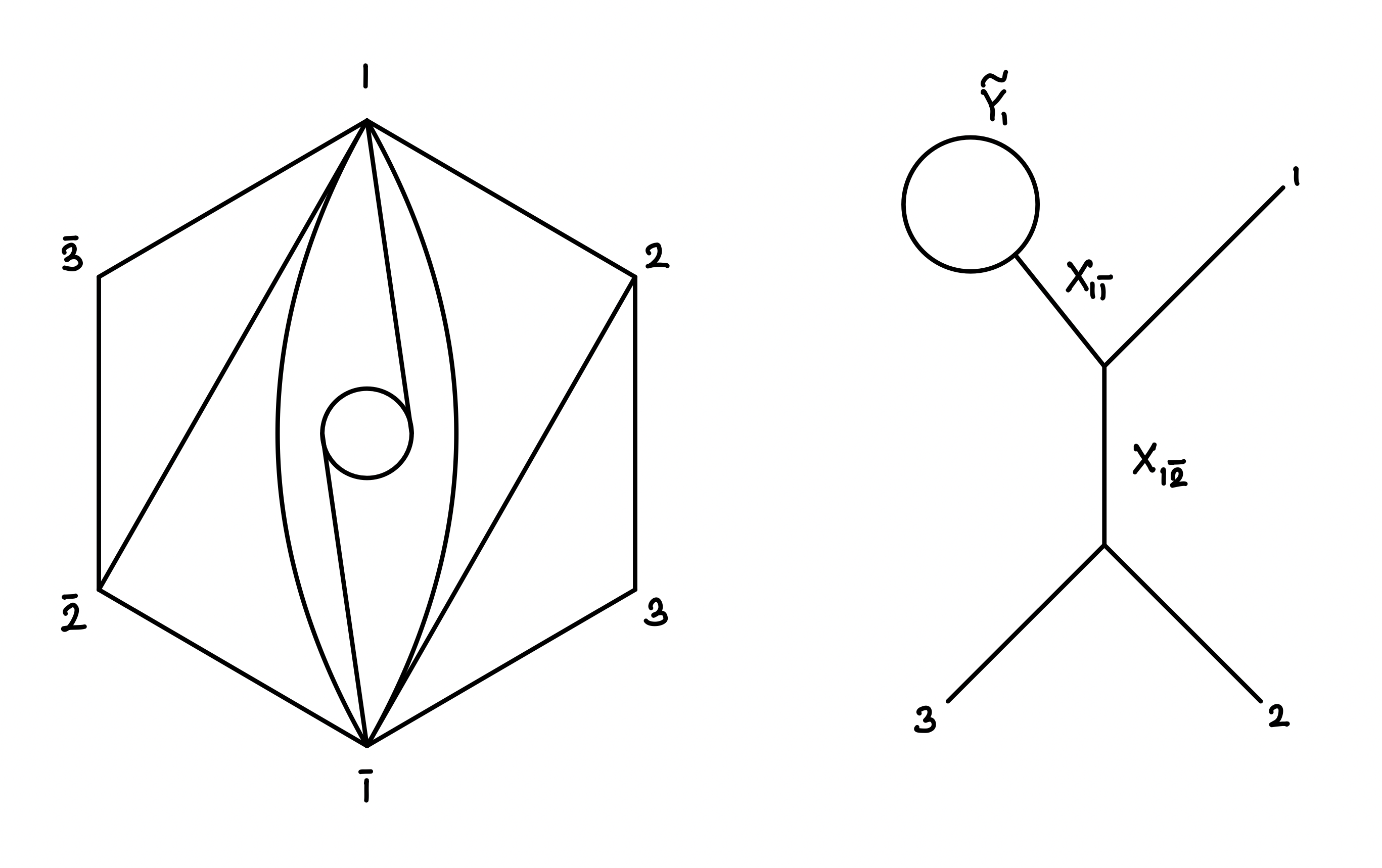
Generically the action of an element of $S_{n}$ on a planar scattering channel takes us to a non-planar scattering channel. However, there is a subgroup of $2^{n-2}$ elements generated by elements like the one depicted in figure 1 that give you back the same scattering channel. More in detail, suppose $\sigma_{S}$ is an element of $S_{n}$ that takes a planar diagram $P$ to $S$ when acted by $\sigma_{S}$. That is, $\sigma_{S}\cdot P=S$. Then $\alpha\cdot\sigma_{S}\cdot P=S$ as well, where $\alpha$ is one of the $2^{n-2}$ elements that takes $S$ back to itself. At the same time, there are $n$ order $n$ elements of $S_{n}$, the cyclic permutations, that take you from one planar scattering channel to another planar scattering channel. Therefore, if $\sigma_{P,P^{\prime}}\in C_{n}$ is such that $\sigma_{P,P^{\prime}}\cdot P^{\prime}=P$, where $P^{\prime}$ is planar, then $\alpha\cdot\sigma\cdot\sigma_{P,P^{\prime}}$ takes $P^{\prime}$ to $S$, $\alpha\cdot\sigma\cdot\sigma_{P,P^{\prime}}\cdot P^{\prime}=S$. In other words, for any scattering channel $S$, there are $n2^{n-2}$ elements of $S_{n}$ that take some planar diagram to $S$. This is beautifully captured by the formula relating the total number of distinguished Feynman diagrams with cubic vertices and the Catalan number, which is the number of planar Feynman diagrams.

where $(2n-5)!!$ is the total number of $n$-point tri-valent Feynman diagrams and $C_{n-2}$ is the total number of $n$-point tri-valent planar Feynman diagrams.²² 2 This identity follows trivially from the definitions, $C_{n-2}\,=\,\frac{(2n-4)!}{(n-2)!(n-1)!}$, $(2n-5)!!\,=\,\frac{(2n-4)!}{2^{n-2}(n-2)!}$.

Consider the Cartersian space ${\bf R}^{\frac{n(n-3)}{2}}$. We denote it as ${\cal E}_{n}$, so as to contrast it with the kinematic space of Mandelstam invariants ${\cal K}_{n}$.³³ 3 To be completely precise, ${\cal E}_{n},\,{\cal K}_{n}$ are real projective spaces of dimension $\frac{n(n-3)}{2}$, but we gauge fix the projective freedom by choosing the first co-ordinate to be $1$. We fix once and for all, a basis $\{x_{ij}\,|\,1\,\leq\,i\,<\,j+1\,\leq\,n\,\}$ in ${\cal E}_{n}$. This basis is labelled by chords of an n-gon : $\{\,x_{ij}\,|\,1\leq\,i\,<j+1\,\leq\,n\}$. Let $y_{i_{1},\dots\,i_{k}}\,1\,\leq\,i_{1}\,<\,\dots\,<\,i_{k}\,\leq\,n$ be defined as,

These two equations imply that,

The $(n-3)$-dimensional ABHY associahedron [8] is a specific convex realization of the associahedron $A_{n}$ in the positive quadrant of the embedding space, ${\cal E}_{n}^{\geq\,0}:=\,\{\,x_{ij}\,\geq\,0\,\forall\,(i,j)\,\}$, defined as follows [8, 21, 20]; Given any reference triangulation $T$, consider the intersection of the positive quadrant of the embedding space $\mathcal{E}_{n}^{\geq 0}$ and the hyper-planes given the equations,

For any choice of positive constants $c_{ij}$, we get a polytopal realization of $A_{n}$.

We will denote the ABHY realization by $A_{n}^{T}$ as it explicitly depends on the choice of the reference triangulation. Our review of ABHY realization is based on [20], whereas the original construction in [8] where these polytopes were discovered directly in the kinematic space of Mandelstam invariants ${\cal K}_{n}$. We now quickly review the relationship between the two.

In space-time dimensions $d\,\geq\,n-3$, the kinematic space ${\cal K}_{n}$ spanned by the Mandelstam variables can also be realized as a ${\bf R}^{\frac{n(n-3)}{2}}$ space. This identification involves identifying a (complete) set of Mandelstam invariants with the coordinate basis. A rather convenient choice of co-ordinates is the set of planar kinematic variables $\{\,X_{ij}\,|\,1\,\leq\,i\,<\,j+1\,\leq\,n\,\}$.

In general, given any ordering $\{\,\sigma(1),\,\dots,\,\sigma(n)\,\}$ obtained by action of a permutation $\sigma\,\in\,S_{n}$ on the standard ordering, one can define the so-called $\sigma$-planar variables which are labelled by chords of an $n$-gon whose vertices are ordered in clockwise direction as $(\,\sigma(1),\,\dots,\,\sigma(n)\,)$. Any such choice of $\sigma$-planar basis defines for us a linear space ${\cal K}_{n}^{\sigma}$ with $\sigma$-planar variables defining an orthonormal basis.⁴⁴ 4 We note that in ${\cal K}_{n}$, $\sigma$-planar variables do not form the Cartesian basis if $\sigma$ is not a $\{\,i,\,i+1,\,\dots,\,n,\,1,\,\dots,\,i-1\}$. In what follows, we fix once and for all an ordering of $(1,\dots,n)$, and ${\cal K}_{n}$ is defined as the kinematic space in which $X_{ij}$ form an orthonormal coordinate system.

The relationship between ABHY realisation in [8] and [20] is simply the identifcation of ${\cal E}_{n}$ with ${\cal K}_{n}$ by the isometry

This realization has several rather remarkable properties that distinguish it from other realizations of the associahedron, making it the “amplituhedron" for bi-adjoint $\phi^{3}$ theory [8]. Let ${\cal D}$ be the set of all the dissections of an $n$-gon whose vertices are labeled $\{1,\,\dots,\,n\}$ in a clockwise direction.

• •

  All the co-dimension one faces (facets) of $A_{n-3}^{T}$ are in bijection with the set

  $\displaystyle\{\,X_{ij}\,=\,0|(i,j)\,\in\,{\cal D}\,\}$

  which is the set of all the simple poles in the bi-adjoint color-ordered amplitude, ${\cal M}_{n}(\,(1,\dots,n)\,|\,(1,\dots,n)\,)$.

• •

  For a $n$ dimensional associahedron, precisely $[\frac{n}{2}]$ pairs of co-dimension one faces are parallel to each other.

• •

  On a facet of $A_{n-3}^{T}$ which corresponds to $X_{ij}\,=\,0$ for some $(i,j)\,\in\,{\cal D}$, $X_{mn}\,>0$ $\forall\,(m,n)\,\in\,{\cal D}$ such that $(m,n)\,\cap\,(i,j)\,\neq\,0$.

For later purposes, we also recall that $A_{n-3}$ also induces a unique projective $(n-3)$-form on ${\cal E}_{n}$.

The projectivity is the invariance of $\Omega^{{\cal E}_{n}}_{n-3}$ under $x_{ij}\,\rightarrow\,f(\{x_{mn}\})\,x_{ij}$ for any function $f$. As ABHY proved, under the identification of ${\cal E}_{n}$ with ${\cal K}_{n}$ $A_{n-3}^{T}$ is the positive geometry for bi-adjoint tree-level S matrix as

In this paper, we use these ideas to look for positive geometries in ${\cal K}_{n}$ which generate the S-matrix of (massive or massless) $\phi^{3}$ theory without color in $D\,\geq\,n$ dimensions. That is, our goal is to discover a set of linear maps from ${\cal E}_{n}\,\rightarrow\,{\cal K}_{n}$ such that the resulting image of the ABHY associahedron in ${\cal K}_{n}$ constitute a family of polytopes whose co-dimension one facets exhaust all the poles of the tree-level S matrix with cubic interaction.

We now review the discovery of a family of polytopes known as Permutahedra in the kinematic space whose canonical form has poles at $\{\,s_{1\sigma(2)\,\dots\,\sigma(i)}\,|\,2\,\leq\,i\,\leq\,n-1\,|\,\sigma\,\in\,S_{n-2}\,\}$.

Starting from the seminal work in [8], it has been realized that a simple polytope whose vertex set is bijection with the set of poles defined above is the permutahedron ${\cal P}_{n}$ [8, 25]. This is because, as we review below, ${\cal P}_{n}$ is a combinatorial polytope whose vertex set is in bijection with $S_{n-2}$, [26]

Permutahedron can be defined as follows; ⁵⁵ 5 In the interest of brevity, we are paraphrasing the definition such that it relates to the primary question under investigation. Given a set $I\,=\,\{1\,\dots,\,n\}$, we fix two elements, say $i,\,i+1$ as the “initial" and “final" vertices and “rotate $I$" to

Let

We now consider the configuration space defined as

We now define a permutahedron ${\cal P}_{n}^{i+1,i}$ as a simple polytope whose vertex set is in bijection with $\sigma\,\cdot I$ and two vertices are adjacent if and only if they are related by a $\sigma$ which exchanges $(m,n)\,\rightarrow\,(n,m)\,|\,(m,n)\,\in\,I_{i}$. ${\cal P}_{n}$ has several interesting properties.

1. 1.

   It is a simple polytope with the dimensionality given by the number of propagators in a tri-valent Feynman graph, $n-3$

2. 2.

   It is a member of the family of polytopes known as Cayley polytopes with the largest number ($(n-2)!$) of vertices among this family.

3. 3.

   Given a planar ordering, Each permutahedron has precisely one vertex that corresponds to the planar channel, and all the other vertices correspond to non-planar Feynman diagrams.

4. 4.

   No vertex of ${\cal P}_{n}^{i+1,i}$ corresponds to the set of propagators of the type

   $\displaystyle\{\,(i+1,\sigma(i+2)),\,(\sigma(i+3),\,\sigma(i+4)),\,\dots,\,(\sigma(i-1),i)\,\}$

In [8], Arkani-Hamed, Bai, He, and Yan, in fact, constructed a convex realization of the Permutahedron in ${\cal K}_{n}$ as follows.

Given ${\cal P}_{n}^{i+1,i}$, consider a positive orthant in ${\cal K}_{n}$ defined using the following inequalities.

The set of constraints whose intersection with this positive orthant maps out the generalized permutahedron are simply,

The canonical form on the convex ${\cal P}_{n}^{i+1,i}$ is,

which is a partial contribution to the S-matrix of $\phi^{3}$ theory. In a beautiful paper [25], Nick Early analyzed these realizations in further detail and proved that they are, in fact, equivalent to a class of simple polytopes called zonotopal generalized permutahedra which were discovered by A. Postnikov [26].⁶⁶ 6 This relationship was already anticipated by the authors in [8].

In spite of the remarkable richness contained in these geometries (see, e.g.[9]) as well as the fact that each such ${\cal P}_{n}^{i+1,i}$ has precisely one planar and the rest non-planar channels as vertices, a precise relationship between zonotopal generalized permutahedra and the S-matrix of ordinary $\phi^{3}$ theory remains to be understood. Property (4) stated above only adds a further layer of mystery in the role permutahedra may play in unraveling the structure of S-matrix without color.

We will not consider these mythical objects in our work and will instead show how to recover all the poles (planar as well as non-planar) of the S matrix from a set of incarnations of the ABHY associahedron located in various quadrants of ${\cal K}_{n}$.

In this section, we define a family of maps between the embedding space ${\cal E}_{n}$ and the kinematic $\mathcal{K}_{n}$ space parameterized by the Bose symmetry reviewed in section 2. Given an element $\sigma\in S_{n}$ we consider the following linear isomorphism, ⁷⁷ 7 In [8] $s_{\sigma(i)\sigma(i+1)\ldots\sigma(j-1)}$ were called the $\sigma$-planar variables $X_{\sigma(i)\sigma(j)}$.

As we have fixed the basis in both, ${\cal K}_{n}$ and ${\cal E}_{n}$, each such map $f_{\sigma}$ is a matrix in $GL(\frac{n(n-3)}{2})$.

The linear isomorphism $f_{\sigma}$ defined in (4.1) maps the ABHY associahedra $A_{n}^{T}$ in the (positive quadrant of) the embedding space to a geometric realization of associahedra in kinematic space $\mathcal{K}_{n}$. Given a triangulation $T$ of an $n$-gon and an element $\sigma\in S_{n}$, we get such a geometric realization of associahedra. We denote this geometric realization as $A_{n}^{T,\sigma}$.

More in detail, as discussed in section 3, given a triangulation, we have a geometric realization of associahedra by considering the intersection of hyper-planes given in equation (3.4) with the positive quadrant of the embedding space. Now the linear isomorphism $f_{\sigma}$ maps the hyper-planes to the hyper-planes

While the positive quadrant of the embedding space $\mathcal{E}_{n}^{\geq 0}$ is mapped to what we call $\sigma$-positive region $\mathcal{K}_{n}^{\sigma\geq 0}\subset\mathcal{K}_{n}$. The $\sigma$-positive region is given by

The intersection of hyper-planes given by (4.3) and the $\sigma$-positive region $\mathcal{K}_{n}^{\sigma\geq 0}$ gives us the geometric realization $A_{n}^{T,\sigma}$.

We now expand on several characteristics of $A_{n}^{T,\sigma}$ for generic $\sigma\in S_{n}$, which reveal the similarities and differences of this geometry with the ABHY realization.

• •

  The set $F_{\sigma}$ of all the co-dimension one boundaries of $A_{n}^{T,\sigma}$ are in bijection with the following set of poles,

  $\displaystyle F_{\sigma}\,\overset{1-1}{=}\,\{\,s_{\sigma(i),\,\dots,\,\sigma(j-1)}\,|\,1\leq\,i\,<j-1\,\leq\,n\,\}$

  (4.5)

• •

  It is important to note that $F_{\sigma}$ is in bijection with the set of poles of the color ordered amplitude in bi-adjoint $\phi^{3}$ theory with the ordering $(\sigma(1),\,\dots,\,\sigma(n)\,|\,\sigma(1),\,\dots,\,\sigma(n)\,)$. However, one crucial difference with the bi-adjoint case is worth emphasizing: The kinematic space in the case of bi-adjoint color ordered amplitude is defined via the $\sigma$-planar kinematic variables, $X_{\sigma(i),\sigma(j)}$ (for a given a color order defined by a representative $\sigma$), [8]. In contrast, in the present case where the external states have no color, ${\cal K}_{n}$ is fixed once and for all. Our goal is to prove that the complete tree-level S matrix is given by $n-3$ forms on ${\cal K}_{n}$.

• •

  As the following lemma proves, the union over all the deformed realisations of $A_{n-3}$ is a positive geometry, [17].

References

- [1] Mrunmay Jagadale and Alok Laddha. Towards positive geometry of multi scalar field amplitudes. Accordiohedron and effective field theory. JHEP, 04:100, 2022.
- [2] Mrunmay Jagadale and Alok Laddha. Towards Positive Geometries of Massive Scalar field theories. arxiv : 2206.07979, hep-th, 6 2022.
- [3] Nima Arkani-Hamed and Jaroslav Trnka. The Amplituhedron. JHEP, 10:030, 2014.
- [4] Livia Ferro and Tomasz Łukowski. Amplituhedra, and beyond. Journal of Physics A: Mathematical and Theoretical, 54(3):033001, dec 2020.
- [5] Enrico Herrmann and Jaroslav Trnka. The SAGEX Review on Scattering Amplitudes, Chapter 7: Positive Geometry of Scattering Amplitudes, 3 2022.
- [6] Andrew Hodges. Eliminating spurious poles from gauge-theoretic amplitudes. Journal of High Energy Physics, 2013(5):135, 2013.
- [7] N. Arkani-Hamed, J. Bourjaily, F. Cachazo, A. Hodges, and J. Trnka. A note on polytopes for scattering amplitudes. Journal of High Energy Physics, 2012(4):81, 2012.
- [8] Nima Arkani-Hamed, Yuntao Bai, Song He, and Gongwang Yan. Scattering Forms and the Positive Geometry of Kinematics, Color and the Worldsheet. JHEP, 05:096, 2018.
- [9] Song He and Chi Zhang. Notes on Scattering Amplitudes as Differential Forms. JHEP, 10:054, 2018.
- [10] Pinaki Banerjee, Alok Laddha, and Prashanth Raman. Stokes polytopes: the positive geometry for interactions. JHEP, 08:067, 2019.
- [11] Prashanth Raman. The positive geometry for interactions. JHEP, 10:271, 2019.
- [12] Aidan Herderschee and Fei Teng. Open associahedra and scattering forms. JHEP, 12:134, 2020.
- [13] Aidan Herderschee, Song He, Fei Teng, and Yong Zhang. On Positive Geometry and Scattering Forms for Matter Particles. JHEP, 06:030, 2020.
- [14] Giulio Salvatori and Stefan Stanojevic. Scattering Amplitudes and Simple Canonical Forms for Simple Polytopes. JHEP, 03:067, 2021.
- [15] Nikhil Kalyanapuram. Stokes Polytopes and Intersection Theory. Phys. Rev. D, 101(10):105010, 2020.
- [16] P. B. Aneesh, Pinaki Banerjee, Mrunmay Jagadale, Renjan Rajan, Alok Laddha, and Sujoy Mahato. On positive geometries of quartic interactions: Stokes polytopes, lower forms on associahedra and world-sheet forms. JHEP, 04:149, 2020.
- [17] David Damgaard, Livia Ferro, Tomasz Łukowski, and Robert Moerman. Kleiss-kuijf relations from momentum amplituhedron geometry. Journal of High Energy Physics, 2021(7):111, 2021.
- [18] Severin Barmeier, Prafulla Oak, Aritra Pal, Koushik Ray, and Hipolito Treffinger. Towards a categorification of scattering amplitudes. arXiv, 2112.14288 hep-th, 12 2021.
- [19] Freddy Cachazo and Bruno Giménez Umbert. Connecting Scalar Amplitudes using The Positive Tropical Grassmannian. arxiv : 2205.02722, hep-th, 5 2022.
- [20] Arnau Padrol, Yann Palu, Vincent Pilaud, and Pierre-Guy Plamondon. Associahedra for finite type cluster algebras and minimal relations between -vectors. arXiv: Representation Theory, 2019.
- [21] Véronique Bazier-Matte, Nathan Chapelier-Laget, Guillaume Douville, Kaveh Mousavand, Hugh Thomas, and Emine Yıldırım. ABHY Associahedra and Newton polytopes of -polynomials for finite type cluster algebras, 8 2018.
- [22] David Damgaard, Livia Ferro, Tomasz Łukowski, and Robert Moerman. Momentum amplituhedron meets kinematic associahedron. Journal of High Energy Physics, 2021(2):41, 2021.
- [23] Tomasz Łukowski, Robert Moerman, and Jonah Stalknecht. Pushforwards via scattering equations with applications to positive geometries. Journal of High Energy Physics, 2022(10):3, 2022.
- [24] Nima Arkani-Hamed, Hadeleigh Frost, Pierre-Guy Plamondon, Giulio Salvatori, and Hugh Thomas. Clusterohedra and all loop S-matrix. In preparation.
- [25] Nick Early. Generalized permutohedra in the kinematic space. arXiv 1804.05460 math.CO, 4 2018.
- [26] Alexander Postnikov. Permutohedra, associahedra, and beyond. arXiv Mathematics e-prints, page math/0507163, July 2005.
- [27] Freddy Cachazo, Song He, and Ellis Ye Yuan. Scattering of Massless Particles: Scalars, Gluons and Gravitons. JHEP, 07:033, 2014.
- [28] P. B. Aneesh, Mrunmay Jagadale, and Nikhil Kalyanapuram. Accordiohedra as positive geometries for generic scalar field theories. Phys. Rev. D, 100(10):106013, 2019.
- [29] Frédéric Chapoton. Stokes posets and serpent nests. Discrete Mathematics & Theoretical Computer Science, Vol. 18 no. 3, 2016.
- [30] Thibault Manneville and Vincent Pilaud. Geometric realizations of the accordion complex of a dissection. Discrete & Computational Geometry, 61:507–540, 2019.
- [31] Ryota Kojima. Weights and recursion relations for tree amplitudes from the positive geometry. JHEP, 08:054, 2020.
- [32] Renjan Rajan John, Ryota Kojima, and Sujoy Mahato. Weights, Recursion relations and Projective triangulations for Positive Geometry of scalar theories. JHEP, 10:037, 2020.
- [33] Giulio Salvatori. 1-loop amplitudes from the halohedron. Journal of High Energy Physics, 2019(12):74, 2019.
- [34] Nima Arkani-Hamed, Song He, Giulio Salvatori, and Hugh Thomas. Causal Diamonds, Cluster Polytopes and Scattering Amplitudes, 12 2019.
- [35] Cesar Ceballos and Vincent Pilaud. Cluster algebras of type d: Pseudotriangulations approach. Electron. J. Comb., 22:P4.44, 2015.
- [36] G Dian, P Heslop, and A Stewart. Internal boundaries of the loop amplituhedron. [arXiv:2207.12464 [hep-th]], 2022.