UTF8mc
Defense-Prefix for Preventing Typographic Attacks on CLIP
Abstract
Vision-language pre-training models (VLPs) have exhibited revolutionary improvements in various vision-language tasks. In VLP, some adversarial attacks fool a model into false or absurd classifications. Previous studies addressed these attacks by fine-tuning the model or changing its architecture. However, these methods risk losing the original model’s performance and are difficult to apply to downstream tasks. In particular, their applicability to other tasks has not been considered. In this study, we addressed the reduction of the impact of typographic attacks on CLIP without changing the model parameters. To achieve this, we expand the idea of “class-prefix learning” and introduce our simple yet effective method: Defense-Prefix (DP), which inserts the DP token before a class name to make words “robust” against typographic attacks. Our method can be easily applied to downstream tasks, such as object detection, because the proposed method is independent of the model parameters. Our method significantly improves the accuracy of classification tasks for typographic attack datasets, while maintaining the zero-shot capabilities of the model. In addition, we leverage our proposed method for object detection, demonstrating its high applicability and effectiveness. The codes and datasets are available at https://github.com/azuma164/Defense-Prefix.
1 Introduction
In recent years, vision-language pre-training models (VLPs) such as CLIP [34] and ALIGN [20] have revolutionized downstream vision-language tasks such as classification [5, 47, 13], object detection [48, 12], segmentation [50, 51], and image generation [35, 38, 6]. Such models are trained on web-scale data, for example, 400 million text-image pairs in the case of CLIP. The rich supervision provided by natural language enabled these pre-trained models to achieve impressive results on various downstream tasks with little or no additional training data.
However, some adversarial attacks [21, 14] can fool such models into making false or absurd classifications. Goh et al. [14] found that CLIP is vulnerable to typographic attacks, in which the text in an image results in misclassification. In Fig. 1, the yellow tag that states “mouse” causes CLIP to misclassify the dog as a mouse.

As described below, we found that downstream classifiers built based on CLIP for different tasks are also susceptible to typographic attacks. Therefore, defense methods against such attacks should be readily applied to other downstream tasks. However, previous studies [19, 31] have mainly focused on typographic attacks on classification and ignored their applicability. Materzynska et al. [31] learned a transformation module on top of the CLIP output and PAINT [19] fine-tuned the model. Since these methods change the model parameters, they risk losing the original model’s performance and are difficult to apply to downstream tasks. Additionally, if you calculate the image features of CLIP beforehand, these approaches require updating those features.
To solve these problems, we propose a simple yet effective defense method: Defense-Prefix (DP), which inserts the DP token before a class name. The DP token is a unique token followed by a class name (e.g., “a photo of a [DP] dog”). An image feature from Fig. 1(a) would resemble a text feature from “a photo of a mouse”, but would not be similar to a feature from “a photo of a [DP] mouse”. In other words, DP makes the class name “robust” against the attacks. Learning a unique token followed by a class name has been primarily conducted in subject-driven image generation [37, 25, 26]. We define this approach as class-prefix learning and apply the concept of class-prefix learning to prevent typographic attacks.
Our approach learns only the word embedding vector for the DP token. Therefore, we do not update the original CLIP. After the DP vector is obtained, it can be used for any task. This simplicity is a significant advantage over existing works because all other works require training the model.
We experimentally demonstrate the effectiveness of the proposed method. (1) We first conduct experiments on classification using ten synthetic and three real-world typographic attack datasets. Here, due to the insufficient number of datasets, we create the biggest Real-world Typographic Attack dataset “RTA-100”, which contains 100 categories and 1000 images. Compared with CLIP, our method effectively prevents typographic attacks (e.g., +9.61% on synthetic and +17.70% on real-world datasets), while losing only 0.64% on average for original datasets. (2) We also evaluate our method on object detection by using RegionCLIP [48]. The proposed method does not require additional training because only the input of the text encoder is modified. Our results indicate that the downstream classifiers based on CLIP are also susceptible to typographic attacks. Our method reduces the impact of the attacks (e.g., +16.0 AP50 on COCO, +6.2 mAP on LVIS), while keeping the original accuracy (e.g., +0.1 AP50 on COCO, -0.3 mAP on LVIS).
In summary:
- •
We expand class-prefix learning and propose DP, a novel method for preventing typographic attacks on CLIP without changing the model parameters.
- •
We find downstream classifiers built based on CLIP are also vulnerable to typographic attacks.
- •
Our method effectively prevents typographic attacks, while keeping the original model’s performance. In addition, we demonstrate the easy application of our approach to downstream tasks.
- •
We creat the biggest real-world typographic attack dataset RTA-100, which will be publicly available.
2 Related work
2.1 Vision-language pre-training (VLP)
Learning the joint vision-language representation space has been of great interest in the field of computer vision. Recently, CLIP [34] and ALIGN [20] collected million/billion-scale image-caption pairs from the Internet and learned to match images with image descriptions. These models obtain a strong vision-language representation space, which has been extremely effective for downstream tasks.
Recent studies have transferred the knowledge of these models to downstream recognition tasks, such as classification [5, 47, 13], object detection [48, 12], semantic segmentation [51, 50], panoptic segmentation [8], and multi-label recognition [44]. Typically, these methods freeze a VLP text encoder and then use it directly. Therefore, the proposed method can be applied without additional training.
2.2 Typographic attacks
CLIP is known to be weak against typographic attacks [14, 1]. Goh et al. [14] found that the text in an image results in misclassification of CLIP as shown in Fig. 1.
Materzynska et al. [31] applied the learned linear transformation to the CLIP output to disentangle the visual concept from the spelling capabilities of CLIP. Ilhalco et al. [19] interpolated the weights of the parameters between the fine-tuned and the original CLIP models to prevent typographic attacks. These methods risk losing the original model’s performance and are difficult to apply to downstream tasks. Also, they need to update the image features.
Unlike these methods, our method does not modify the architecture or model parameters. In addition, our method does not update the image features.
2.3 Prompt learning in VLP
Inspired by the success in NLP [43, 22, 49], to adapt VLP to downstream tasks, several studies have learned prompt tokens in end-to-end training. CoOp [53] first utilized prompt learning in VLP to improve the accuracy of classification tasks. This was followed by other studies [52, 30, 23]. Recently, some studies [44, 50, 12, 51, 10] have focused on using prompt learning to improve other downstream recognition tasks apart from classification.
Prompt learning trains tokens of the whole sentence except for a class name, whereas our class-prefix learning trains one token before a class name. Tokens obtained by class-prefix learning can be used for any task that uses prompts to input text, whereas prompt learning must be trained only for the specific recognition task and cannot be used for any other task.
2.4 Class-prefix learning
We define the approach for learning a unique token followed by a class name as class-prefix learning. Class-prefix learning has been mainly conducted in the research of image generation [37, 25, 26, 40]. Ruiz et al. [37] addressed a new problem: subject-driven generation. They learned a unique identifier followed by the class name of the subject (e.g., “A [V] dog”). They aimed to synthesize novel scenes of the subject in different contexts while keeping its key visual features.
Apart from image generation, class-prefix learning has rarely been investigated. Because class-prefix learning retains the original input texts, it can be incorporated into various vision-language tasks. In this study, we propose a novel method for learning a prefix to prevent typographic attacks.

3 Method
3.1 Preliminaries: CLIP
We first introduce CLIP [34] as the basis for our approach. It consists of two encoders: an image encoder and a text encoder. CLIP encodes the images and text in the same embedding space. The image encoder can be either ResNet [17] or Vision-Transformer [9]. The text encoder is Transformer [45]. To encode an input text, such as “a photo of a dog”, CLIP first converts each word to a -dimensional word embedding vector ( represents the dimension of a word embedding vector), using a learned vocabulary. Subsequently, the word embedding vectors are fed into the transformer to obtain the final text feature.
The CLIP can be used for zero-shot image recognition. Let us consider -class image recognition problem. Let be an image feature generated by the image encoder ( represents the dimension of a feature vector) and be a set of text features produced by the text encoder. Here, represents the -th category.
In particular, each is derived from a text prompt based on a template such as “a photo of a <CLS>.”, where <CLS> can be replaced with the -th class name. The prediction probability that the output label is of class is then
| (1) |
where calculates the cosine similarity and is a temperature parameter learned by CLIP.
3.2 Defense-Prefix
In this section, we present the proposed approach. Our goal is to train the word embedding vector for the DP token, i.e., a single -dimensional vector. We define this word embedding vector as the DP vector. Here, none of the model parameters are modified. Given the -th class name, we define the input sequence of words (text prompts) as . We also prepare , which contains the DP token.
| (2) | |||||
| (3) |
Here, and represent the DP token and -th class name, respectively, while form a template of words. For example, in the case “a photo of a <CLS>.”, is “a” and is “photo”. As aforementioned, CLIP converts each word into a -dimensional word embedding vector using the learned vocabulary as follows:
| (4) | |||||
| (5) |
where denote the learned word embedding vectors. The vectors are pre-trained and fixed. Here, we aim to learn the DP vector (), which is a word embedding vector for the DP token.
Then, we enter and into the text encoder and obtain the original and “robust” class features and , respectively. Here, represents the number of classes and all . We can now recognize an image using Eq. 1 with the original () or the robust () class features. Robust class features reduce the impact of typographic attacks.
The goal is to train the DP vector so that the word next to the DP token is robust against typographic attacks. To achieve this, we propose using defense loss and identity loss (Fig. 2). Defense loss enables the DP token to prevent typographic attacks, and identity loss helps it maintain the original meanings of the class names. For the training, we assume that a set of image pairs, comprising original and “attack” images, is available. The attack image is obtained by synthesizing the incorrect label text on the original image. We calculate defense loss and identity loss for each pair.
Defense loss:
The defense loss aims to prevent typographic attacks. To achieve this, we adopt the cross-entropy loss in the same manner as for ordinary classification tasks. Let and represent the original and attack images, respectively. For example, and show an image of a dog and the same image of the same dog but with a synthesized text “bird”, respectively. We then obtain the image feature by applying to the image encoder. We classify the typographic attack image using robust class features as follows:
| (6) |
We minimize the standard classification loss based on the cross-entropy to train the DP vector. The defense loss for is computed as follows:
| (7) |
where is a one-hot vector representing the ground truth.
Identity loss:
The identity loss function aims to help the learned token maintain the original meanings of the words. To achieve this goal, we ensure a consistent output with and without DP tokens. To distill the knowledge of CLIP, some studies [15, 28] have used the output features of CLIP. However, how to use text features for distillation in our method is unclear. Then, we utilize classification results. First, we classify the original image using the original () and robust () class features as follows:
| (8) |
| (9) |
where denotes the image feature from . Here, we make the probability distribution of approach that of using KL-divergence. Formally, the identity loss for is defined as:
| (10) |
where is a one-hot vector (-th element is one). DP maintains the performance of the original model by mimicking the original classification results.
Finally, the loss for the image pair is computed as:
| (11) |
where is a hyperparameter that balances the losses. Empirically, we set .
4 Experiments
4.1 Training Defense-Prefix
First, we train the DP vector. After obtaining the learned DP vector, we apply it to the experiments of recognition tasks in Sec. 4.2 and 4.3. We train the DP vector only in Sec. 4.1.
Datasets:
Implementation details:
We initialize the image and text encoders from the CLIP [34] pre-trained model and keep them frozen during training. For the image encoder, ViT-B/32 and RN50x4 are applied for classification and object detection, respectively. We train only one vector for DP, which is the only learnable part of our method. The DP vector is randomly initialized by drawing from a zero-mean Gaussian distribution with a standard deviation of 0.02. We use SGD optimizer with an initial learning rate of 0.002, which is decayed using the cosine annealing rule. We train the DP vector for 10 epochs with a batch size of 512, using one NVIDIA V100.
4.2 Classification
In this section, we evaluate the performance of the proposed method based on the classification tasks. We compare our method to CLIP [34], Materzynska et al. [31], and PAINT [19].
Datasets:
We employ ten publicly available image classification datasets used in CLIP: ImageNet [7], Caltech101 [11], OxfordPets [33], StanfordCars [24], Flowers102 [32], Food101 [2], FGVCAircraft [29], DTD [4], SUN397 [46], EuroSAT [18]. To evaluate the classification of typographic attack datasets, we create synthetic typographic attack datasets using those ten datasets (Fig. 3: left). Also, we use two publicly available real-world typographic attack datasets from Materzynska et al. [31] and PAINT. In addition, due to the insufficient number of datasets, we generate our real-world attack dataset RTA-100 (Fig. 3: right). For real-world attack datasets, we use class labels of objects and labels of tags as the candidate categories.
RTA-100:
As described before, we create the biggest real-world typographic attack dataset RTA-100, which contains 100 categories and 1000 images. The dataset from Materzynska et al. [31] comprises 19 categories and 171 images, and that from PAINT [19] has 89 categories and 110 images. Combining those datasets is not sufficient to verify the diversity. To increase the test data, we created RTA-100 (see Appendix for more details).
Implementation details:
We use ViT-B/32 for the image encoder. When we evaluate our method on classification, we place the DP token before the class names.

Baselines:
To evaluate the effectiveness of the proposed method, we compare it with the following baselines: CLIP [34], Materzynska et al. [31], and PAINT [19]. Materzynska et al. [31] apply the learned linear layer to the CLIP output. For Materzynska et al. [31], we use a publicly available pre-trained linear layer for ViT-B/32. This linear layer was trained using ImageNet-1K and 182,329 English words. We apply the linear layer to the output of both the image and text encoders of CLIP. For PAINT, we fine-tune the image encoder of CLIP using typographic attack images from ImageNet-100, which is used to train the DP vector. We then interpolate the weights between the fine-tuned image encoder and the original image encoder with , where is the mixing coefficient (). We get patched model as follows: .
| Retain | Typographic attack | ||||
|---|---|---|---|---|---|
| Method | Models | Original | Synth. | Real | Avg. |
| CLIP | - | 61.55 | 34.59 | 46.82 | 40.71 |
| Materzynska+ [31] | 49.50 | 37.44 | 63.61 | 50.53 | |
| PAINT [19] | 59.63 | 49.93 | 55.00 | 52.47 | |
| Ours | 60.91 | 44.20 | 64.52 | 54.36 | |
| Synth. | Real | |||||||||
| Method | Retain models | ImageNet | Caltech | Pets | Cars | ∗Avg. | from [31] | from [19] | RTA-100 | Avg. |
| CLIP | - | 39.10 | 63.97 | 58.95 | 21.02 | 34.59 | 43.27 | 50.00 | 47.20 | 46.82 |
| Materzynska+ [31] | 44.91 | 74.73 | 63.61 | 15.79 | 37.44 | 77.78 | 55.45 | 57.60 | 63.61 | |
| PAINT [19] | 55.9 | 83.57 | 76.53 | 33.44 | 49.93 | 53.22 | 58.18 | 53.60 | 55.00 | |
| Ours | 49.83 | 79.54 | 72.88 | 28.64 | 44.20 | 71.93 | 63.64 | 58.00 | 64.52 | |
Results:
Table 1 summarizes the performance of our method on classification. As previous research [14] has shown, our results demonstrate that text in images harms the original performance of CLIP (e.g., from 61.55% to 34.59% on average). Compared with CLIP, our method improves the performance on all typographic attack datasets (e.g., from 34.59% to 44.20% on synthetic and from 46.82% to 64.52% on real-world datasets), losing little average accuracy on the original datasets (e.g., from 61.55% to 60.91%).
Compared to Materzynska et al., our method exhibits improved performance on both synthetic and real-world typographic attack datasets (e.g., from 37.44% to 44.20% on synthetic and from 63.61% to 64.52% on real-world datasets). When compared with PAINT, our method loses on synthetic attack datasets (e.g., from 49.93% to 44.20% on average), while it significantly improves the performance on real-world attack datasets (e.g., from 55.00 to 64.52 on average). The result indicates that our method is more robust against changes in the appearance of text.
Tables C and 3 present the specific performance in classifying original datasets, and typographic attack datasets, respectively.
Overall, our simple method effectively prevents typographic attacks (e.g., +9.61% on synthetic and +17.70% on real-world typographic attack datasets), while losing the least original accuracy (e.g., -0.64% on average). Although our method does not update CLIP, our simple method of putting the learned prefix before the class names works effectively, even when compared to previous studies. Here, it is worth noting that PAINT must retrain the CLIP encoder and recompute the CLIP features for all images to achieve typographic defense. In contrast, our approach does not need to modify the encoder or existing features. This property is a clear advantage; we can apply our method to any CLIP-based application without modification. Therefore, our method is much better than PAINT if the performance is comparable to PAINT.
4.3 Object detection

In this section, we evaluate the applicability of the proposed method to downstream tasks. In particular, we apply our method to RegionCLIP [48], a zero-shot object detection model. In RegionCLIP, the image encoder is fine-tuned from the CLIP image encoder. Therefore, we cannot apply previous methods [31, 19] directly to RegionCLIP because they need to update the model. On the other hand, we can use DP directly, which we train in Sec. 4.1, because it is independent of the parameters of the image encoder.
Datasets:
Implementation details:
We use a pre-trained RegionCLIP model for RN50x4. We keep the model frozen during the inference and only modify the input of the text encoder by placing the DP token before the class names.
Following RegionCLIP, we evaluate two settings: (1) Ground-truth (GT) bounding boxes used as region proposals. (2) Region proposals obtained from RPN [36].
Baselines:
We use RegionCLIP for zero-shot object detection. The model was pre-trained on Conceptual Caption dataset (CC3M) [41] using the concepts parsed from COCO Caption (COCO cap) [3]. RegionCLIP comprises an RPN and an image encoder. First, possible image regions are proposed by RPN. The model then calculates the similarity between the image features of the proposed regions and the text features of the target categories, recognizing the categories within the local image regions.
Results:
| Region | COCO | LVIS | |
| Method | Proposals | AP50 | mAP |
| RegionCLIP | GT | 65.5 | 50.2 |
| RegionCLIP+Ours | GT | 65.6 | 49.9 |
| RegionCLIP | RPN | 29.6 | 11.1 |
| RegionCLIP+Ours | RPN | 29.6 | 11.3 |
| Region | COCO | LVIS | |
| Method | Proposals | AP50 | mAP |
| RegionCLIP | GT | 25.0 | 31.9 |
| RegionCLIP+Ours | GT | 41.0 | 38.1 |
| RegionCLIP | RPN | 11.0 | 5.17 |
| RegionCLIP+Ours | RPN | 14.4 | 6.25 |
Fig. 4 visualizes the results of zero-shot inference of RegionCLIP and RegionCLIP+Ours with GT boxes on the typographic attack COCO dataset. This shows RegionCLIP is also adversely influenced by typographic attacks, although the image encoder is fine-tuned. For example, the car is misclassified as a handbag (Fig. 4: top left). However, RegionCLIP+Ours correctly recognizes the car.
Tables 5 and 5 present the performance of RegionCLIP and RegionCLIP+Ours. When using GT boxes, compared with the original RegionCLIP, our method shows improved performance on COCO and LVIS for the typographic attack datasets (e.g., 41.0 vs. 25.0 on COCO, 38.1 vs. 31.9 on LVIS), keeping the accuracy on the original datasets (e.g., 65.6 vs 65.5 on COCO, 49.9 vs. 50.2 on LVIS). With RPN proposals, our method also improves on the typographic attack datasets (e.g., 14.4 vs. 11.0 on COCO, 6.25 vs. 5.17 on LVIS) without losing the original performance (e.g., 29.6 vs. 29.6 on COCO, 11.3 vs. 11.1 on LVIS).
4.4 Ablation Studies
Effectiveness of our identity loss:
Table 6 lists the effects of the identity loss. We observe that the performance of DP trained without identity loss drops drastically on the original datasets (e.g., from 60.91% to 55.43% on average). Identity loss effectively helps the learned token maintain the original meanings of the words. Although categorical knowledge distillation has not been commonly used in VLP, the distillation works effectively as a regularization term.
| Method | ImageNet | Caltech | Pets | Cars | Flowers | Food | Aircraft | DTD | SUN | SAT | Avg. |
|---|---|---|---|---|---|---|---|---|---|---|---|
| CLIP | 62.02 | 88.64 | 87.35 | 58.72 | 66.32 | 84.14 | 18.99 | 44.57 | 61.74 | 42.98 | 61.55 |
| Ours w/o identity loss | 55.81 | 85.01 | 86.67 | 52.77 | 58.79 | 77.89 | 15.48 | 30.8 | 52.2 | 38.86 | 55.43 |
| Ours w/ identity loss | 62.48 | 89.28 | 87.22 | 57.47 | 63.82 | 83.65 | 19.26 | 40.64 | 61.41 | 43.85 | 60.91 |
| Typographic attack | |||
|---|---|---|---|
| The position | Original | Synth. | Real |
| the beginning | 60.50 | 44.13 | 63.11 |
| the end | 61.09 | 37.82 | 55.69 |
| before class names | 60.91 | 44.20 | 64.52 |
| Typographic attack | |||
|---|---|---|---|
| Number of tokens | Original | Synth. | Real |
| one token | 60.91 | 44.20 | 64.52 |
| two tokens | 59.57 | 43.41 | 60.41 |
| three tokens | 47.3 | 34.23 | 48.07 |
Position of the DP token:
There are many possible positions for the placement of the DP token. These include: at the beginning of a sentence [39], before a class name [37, 25], and at the end of a sentence.
Table 8 shows the effect of the position of DP. We observe that the performance of DP at the beginning and end of the sentence decreases on synthetic and real-world typographic attack datasets. The result indicates that DP works most effectively before a class name.
The number of DP tokens:
Table 8 shows the effect of the number of DP tokens. When we increase the number of DP tokens, the overall classification accuracy drops. The result indicates that the best number of tokens is one for our DP.
Hyperparameters:
In Sec. 3.2, we use hyperparameters . About the value of , we conduct an ablation study. As Table 9 shows, there is no optimal , and we used . Also, when we train defense-prefix with only identity loss, the performance is similar to original CLIP’s score.
| Method | Original | Synth. | Real |
|---|---|---|---|
| CLIP | 61.55 | 34.59 | 46.82 |
| w/o defense loss | 61.72 | 35.19 | 51.16 |
| 60.93 | 45.31 | 63.21 | |
| 61.75 | 44.73 | 62.73 | |
| 60.91 | 44.20 | 64.52 | |
| 61.21 | 44.72 | 64.16 | |
| 61.37 | 44.82 | 64.71 |
5 Conclusion
In this study, we tackled reducing the impact of typographic attacks on CLIP. To achieve this, we proposed Defense-Prefix, a novel method for preventing typographic attacks on CLIP. We explored the application of class-prefix learning, which is primarily conducted in subject-driven image generation. To maintain the generalization ability of CLIP, we used categorical knowledge distillation as a regularization loss. This helped the learned prefix maintain the original meanings of the words. Although our method did not require updating CLIP, it effectively prevented typographic attacks on CLIP, while keeping the model’s original performance. In addition, we demonstrated that our approach could be easily applied to downstream tasks such as object detection. This is a significant advantage over the existing studies, which require a modification of the model.
Future work & limitation
Our method loses to the previous study on synthetic typographic attack datasets. In addition, we only addressed the problem of typographic attacks. We believe that the proposed method can be applied to other adversarial attacks on VLP. We hope that this work will shed light on research on the utilization of VLP.
References
- [1] Omri Avrahami, Dani Lischinski, and Ohad Fried. Blended diffusion for text-driven editing of natural images. CVPR, 2022.
- [2] Lukas Bossard, Matthieu Guillaumin, and Luc Gool. Food-101 – mining discriminative components with random forests. ECCV, 2014.
- [3] Xinlei Chen, Hao Fang, Tsung-Yi Lin, Ramakrishna Vedantam, Saurabh Gupta, Piotr Dollar, and C. Lawrence Zitnick. Microsoft coco captions: Data collection and evaluation server. arXiv preprint arXiv: 1504.00325, 2015.
- [4] Mircea Cimpoi, Subhransu Maji, Iasonas Kokkinos, Sammy Mohamed, and Andrea Vedaldi. Describing textures in the wild. CVPR, 2014.
- [5] Conde and Turgutlu. CLIP-Art: contrastive pre-training for fine-grained art classification. CVPRW, 2021.
- [6] Katherine Crowson, Stella Biderman, Daniel Kornis, Dashiell Stander, Eric Hallahan, Louis Castricato, and Edward Raff. Vqgan-clip: Open domain image generation and editing with natural language guidance. ECCV, 2022.
- [7] Jia Deng, Wei Dong, Richard Socher, Li-Jia Li, Kai Li, and Li Fei-Fei. ImageNet: A large-scale hierarchical image database. CVPR, 2009.
- [8] Zheng Ding, Jieke Wang, and Zhuowen Tu. Open-vocabulary panoptic segmentation with maskclip. arXiv preprint arXiv: 2208.08984, 2022.
- [9] Alexey Dosovitskiy, Lucas Beyer, Alexander Kolesnikov, Dirk Weissenborn, Xiaohua Zhai, Thomas Unterthiner, Mostafa Dehghani, Matthias Minderer, Georg Heigold, Sylvain Gelly, Jakob Uszkoreit, and Neil Houlsby. An image is worth 16x16 words: Transformers for image recognition at scale. ICLR, 2021.
- [10] Yu Du, Fangyun Wei, Zihe Zhang, Miaojing Shi, Yue Gao, and Guoqi Li. Learning to prompt for open-vocabulary object detection with vision-language model. CVPR, 2022.
- [11] Li Fei-Fei, Rob Fergus, and Pietro Perona. Learning generative visual models from few training examples: An incremental bayesian approach tested on 101 object categories. CVPR, 2004.
- [12] Chengjian Feng, Yujie Zhong, Zequn Jie, Xiangxiang Chu, Haibing Ren, Xiaolin Wei, Weidi Xie, and Lin Ma. Promptdet: Towards open-vocabulary detection using uncurated images. ECCV, 2022.
- [13] Peng Gao, Shijie Geng, Renrui Zhang, Teli Ma, Rongyao Fang, Yongfeng Zhang, Hongsheng Li, and Yu Qiao. CLIP-Adapter: Better Vision-Language models with feature adapters. arXiv preprint arXiv: 2110.04544, 2021.
- [14] Gabriel Goh, Nick Cammarata, Chelsea Voss, Shan Carter, Michael Petrov, Ludwig Schubert, Alec Radford, and Chris Olah. Multimodal neurons in artificial neural networks. Distill, 6(3), 2021.
- [15] Xiuye Gu, Tsung-Yi Lin, Weicheng Kuo, and Yin Cui. Open-vocabulary object detection via vision and language knowledge distillation. ICLR, 2022.
- [16] Agrim Gupta, Piotr Dollár, and Ross Girshick. Lvis: A dataset for large vocabulary instance segmentation. CVPR, 2019.
- [17] He, Zhang, Ren, and Sun. Deep residual learning for image recognition. CVPR, 2016.
- [18] Patrick Helber, Benjamin Bischke, Andreas Dengel, and Damian Borth. Eurosat: A novel dataset and deep learning benchmark for land use and land cover classification. IEEE GRSS, 2019.
- [19] Gabriel Ilharco, Mitchell Wortsman, Samir Yitzhak Gadre, Shuran Song, Hannaneh Hajishirzi, Simon Kornblith, Ali Farhadi, and Ludwig Schmidt. Patching open-vocabulary models by interpolating weights. NeurIPS, 2022.
- [20] Chao Jia, Yinfei Yang, Ye Xia, Yi-Ting Chen, Zarana Parekh, Hieu Pham, Quoc V. Le, Yunhsuan Sung, Zhen Li, and Tom Duerig. Scaling up visual and vision-language representation learning with noisy text supervision. ICML, 2021.
- [21] Jinyuan Jia, Yupei Liu, and Neil Zhenqiang Gong. BadEncoder: Backdoor attacks to pre-trained encoders in self-supervised learning. IEEE S&P, 2022.
- [22] Zhengbao Jiang, Frank F. Xu, Jun Araki, and Graham Neubig. How can we know what language models know? TACL, 2020.
- [23] Muhammad Uzair Khattak, Hanoona Rasheed, Muhammad Maaz, Salman Khan, and Fahad Shahbaz Khan. Maple: Multi-modal prompt learning. CVPR, 2023.
- [24] Jonathan Krause, Michael Stark, Jia Deng, and Li Fei-Fei. 3d object representations for fine-grained categorization. CVPR, 2013.
- [25] Nupur Kumari, Bingliang Zhang, Richard Zhang, Eli Shechtman, and Jun-Yan Zhu. Multi-concept customization of text-to-image diffusion. CVPR, 2023.
- [26] Chen-Hsuan Lin, Jun Gao, Luming Tang, Towaki Takikawa, Xiaohui Zeng, Xun Huang, Karsten Kreis, Sanja Fidler, Ming-Yu Liu, and Tsung-Yi Lin. Magic3d: High-resolution text-to-3d content creation. CVPR, 2023.
- [27] Tsung-Yi Lin, Michael Maire, Serge Belongie, Lubomir Bourdev, Ross Girshick, James Hays, Pietro Perona, Deva Ramanan, C. Lawrence Zitnick, and Piotr Dollár. Microsoft coco: Common objects in context. ECCV, 2014.
- [28] Zongyang Ma, Guan Luo, Jin Gao, Liang Li, Yuxin Chen, Shaoru Wang, Congxuan Zhang, and Weiming Hu. Open-vocabulary one-stage detection with hierarchical visual-language knowledge distillation. CVPR, 2022.
- [29] Subhransu Maji, Esa Rahtu, Juho Kannala, Matthew Blaschko, and Andrea Vedaldi. Fine-grained visual classification of aircraft. arXiv preprint arXiv: 1306.5151, 2013.
- [30] Shu Manli, Nie Weili, Huang De-An, Yu Zhiding, Goldstein Tom, Anandkumar Anima, and Xiao Chaowei. Test-time prompt tuning for zero-shot generalization in vision-language models. NeurIPS, 2022.
- [31] Joanna Materzyńska, Antonio Torralba, and David Bau. Disentangling visual and written concepts in CLIP. CVPR, 2022.
- [32] Maria-Elena Nilsback and Andrew Zisserman. Automated flower classification over a large number of classes. ICVGIP, 2008.
- [33] Omkar M Parkhi, Andrea Vedaldi, Andrew Zisserman, and C. V. Jawahar. Cats and dogs. CVPR, 2012.
- [34] Alec Radford, Jong Wook Kim, Chris Hallacy, Aditya Ramesh, Gabriel Goh, Sandhini Agarwal, Girish Sastry, Amanda Askell, Pamela Mishkin, Jack Clark, Gretchen Krueger, and Ilya Sutskever. Learning transferable visual models from natural language supervision. ICML, 2021.
- [35] Aditya Ramesh, Prafulla Dhariwal, Alex Nichol, Casey Chu, and Mark Chen. Hierarchical Text-Conditional image generation with CLIP latents. arXiv preprint arXiv: 2204.06125, 2022.
- [36] Shaoqing Ren, Kaiming He, Ross Girshick, and Jian Sun. Faster r-cnn: Towards real-time object detection with region proposal networks. NeurIPS, 2015.
- [37] Nataniel Ruiz, Yuanzhen Li, Varun Jampani, Yael Pritch, Michael Rubinstein, and Kfir Aberman. DreamBooth: Fine tuning Text-to-Image diffusion models for Subject-Driven generation. CVPR, 2023.
- [38] Chitwan Saharia, William Chan, Saurabh Saxena, Lala Li, Jay Whang, Emily Denton, Seyed Kamyar Seyed Ghasemipour, Burcu Karagol Ayan, S Sara Mahdavi, Rapha Gontijo Lopes, Tim Salimans, Jonathan Ho, David J Fleet, and Mohammad Norouzi. Photorealistic Text-to-Image diffusion models with deep language understanding. NeurIPS, 2022.
- [39] Kuniaki Saito, Kihyuk Sohn, Xiang Zhang, Chun-Liang Li, Chen-Yu Lee, Kate Saenko, and Tomas Pfister. Prefix conditioning unifies language and label supervision. CVPR, 2023.
- [40] Idan Schwartz, Vésteinn Snæbjarnarson, Sagie Benaim, Hila Chefer, Ryan Cotterell, Lior Wolf, and Serge Belongie. Discriminative class tokens for text-to-image diffusion models. arXiv preprint arXiv: 2303.17155, 2023.
- [41] Piyush Sharma, Nan Ding, Sebastian Goodman, and Radu Soricut. Conceptual captions: A cleaned, hypernymed, image alt-text dataset for automatic image captioning. ACL, 2018.
- [42] Ambesh Shekhar. ImageNet100. https://www.kaggle.com/datasets/ambityga/imagenet100. Accessed: 2023-01-10.
- [43] Taylor Shin, Yasaman Razeghi, Robert L. Logan IV, Eric Wallace, and Sameer Singh. AutoPrompt: Eliciting knowledge from language models with automatically generated prompts. EMNLP, 2020.
- [44] Ximeng Sun, Ping Hu, and Kate Saenko. Dualcoop: Fast adaptation to multi-label recognition with limited annotations. NeurIPS, 2022.
- [45] Vaswani, Shazeer, Parmar, and others. Attention is all you need. NeurIPS, 2017.
- [46] Jianxiong Xiao, Krista A Ehinger, James Hays, Antonio Torralba, and Aude Oliva. Sun database: Exploring a large collection of scene categories. IJCV, 2016.
- [47] Renrui Zhang, Rongyao Fang, Peng Gao, Wei Zhang, Kunchang Li, Jifeng Dai, Yu Qiao, and Hongsheng Li. Tip-adapter: Training-free adaption of clip for few-shot classification. ECCV, 2022.
- [48] Yiwu Zhong, Jianwei Yang, Pengchuan Zhang, Chunyuan Li, Noel Codella, Liunian Harold Li, Luowei Zhou, Xiyang Dai, Lu Yuan, Yin Li, et al. Regionclip: Region-based language-image pretraining. CVPR, 2022.
- [49] Zexuan Zhong, Dan Friedman, and Danqi Chen. Factual probing is [mask]: Learning vs. learning to recall. NAACL, 2021.
- [50] Chong Zhou, Chen Change Loy, and Bo Dai. Denseclip: Language-guided dense prediction with context-aware prompting. CVPR, 2022.
- [51] Chong Zhou, Chen Change Loy, and Bo Dai. Extract free dense labels from clip. ECCV, 2022.
- [52] K Zhou, J Yang, C C Loy, and Z Liu. Conditional prompt learning for vision-language models. CVPR, 2022.
- [53] Kaiyang Zhou, Jingkang Yang, Chen Change Loy, and Ziwei Liu. Learning to prompt for Vision-Language models. IJCV, 2022.
Appendix A Prompts
In Sec. 3.2, we use templates to prepare input text and . For training, we randomly choose a template from hand-crafted prompts in each iteration. For hand-crafted, we use 81 prompts: (
‘<CLS>.’,
‘a photo of a <CLS>.’,
‘a bad photo of a <CLS>.’,
‘a photo of many <CLS>.’,
‘a sculpture of a <CLS>.’,
‘a photo of the hard to see <CLS>.’,
‘a low resolution photo of the <CLS>.’,
‘a rendering of a <CLS>.’,
‘graffiti of a <CLS>.’,
‘a bad photo of the <CLS>.’,
‘a cropped photo of the <CLS>.’,
‘a tattoo of a <CLS>.’,
‘the embroidered <CLS>.’,
‘a photo of a hard to see <CLS>.’,
‘a bright photo of a <CLS>.’,
‘a photo of a clean <CLS>.’,
‘a photo of a dirty <CLS>.’,
‘a dark photo of the <CLS>.’,
‘a drawing of a <CLS>.’,
‘a photo of my <CLS>.’,
‘the plastic <CLS>.’,
‘a photo of the cool <CLS>.’,
‘a close-up photo of a <CLS>.’,
‘a black and white photo of the <CLS>.’,
‘a painting of the <CLS>.’,
‘a painting of a <CLS>.’,
‘a pixelated photo of the <CLS>.’,
‘a sculpture of the <CLS>.’,
‘a bright photo of the <CLS>.’,
‘a cropped photo of a <CLS>.’,
‘a plastic <CLS>.’,
‘a photo of the dirty <CLS>.’,
‘a jpeg corrupted photo of a <CLS>.’,
‘a blurry photo of the <CLS>.’,
‘a photo of the <CLS>.’,
‘a good photo of the <CLS>.’,
‘a rendering of the <CLS>.’,
‘a <CLS> in a video game.’,
‘a photo of one <CLS>.’,
‘a doodle of a <CLS>.’,
‘a close-up photo of the <CLS>.’,
‘the origami <CLS>.’,
‘the <CLS> in a video game.’,
‘a sketch of a <CLS>.’,
‘a doodle of the <CLS>.’,
‘a origami <CLS>.’,
‘a low resolution photo of a <CLS>.’,
‘the toy <CLS>.’,
‘a rendition of the <CLS>.’,
‘a photo of the clean <CLS>.’,
‘a photo of a large <CLS>.’,
‘a rendition of a <CLS>.’,
‘a photo of a nice <CLS>.’,
‘a photo of a weird <CLS>.’,
‘a blurry photo of a <CLS>.’,
‘a cartoon <CLS>.’,
‘art of a <CLS>.’,
‘a sketch of the <CLS>.’,
‘a embroidered <CLS>.’,
‘a pixelated photo of a <CLS>.’,
‘itap of the <CLS>.’,
‘a jpeg corrupted photo of the <CLS>.’,
‘a good photo of a <CLS>.’,
‘a plushie <CLS>.’,
‘a photo of the nice <CLS>.’,
‘a photo of the small <CLS>.’,
‘a photo of the weird <CLS>.’,
‘the cartoon <CLS>.’,
‘art of the <CLS>.’,
‘a drawing of the <CLS>.’,
‘a photo of the large <CLS>.’,
‘a black and white photo of a <CLS>.’,
‘the plushie <CLS>.’,
‘a dark photo of a <CLS>.’,
‘itap of a <CLS>.’,
‘graffiti of the <CLS>.’,
‘a toy <CLS>.’,
‘itap of my <CLS>.’,
‘a photo of a cool <CLS>.’,
‘a photo of a small <CLS>.’,
‘a tattoo of the <CLS>.’,
)
In Sec. 4.2, we evaluate our method through classification. For classification, we use hand-crafted prompts (Table A).
| Dataset | Prompt |
|---|---|
| ImageNet | “a photo of a <CLS>.” |
| Caltech101 | “a photo of a <CLS>.” |
| OxfordPets | “a photo of a <CLS>, a type of pet.” |
| StanfordCars | “a photo of a <CLS>.” |
| Flowers102 | “a photo of a <CLS>, a type of flower.” |
| Food101 | “a photo of a <CLS>, a type of food.” |
| FGVCAircraft | “a photo of a <CLS>, a type of aircraft.” |
| DTD | “<CLS> texture.” |
| SUN397 | “a photo of a <CLS>.” |
| EuroSAT | “a centered satellite photo of a <CLS>.” |
| Real-world typographic attack datasets | “a photo of a <CLS>.” |
Appendix B Synthetic typographic attack datasets

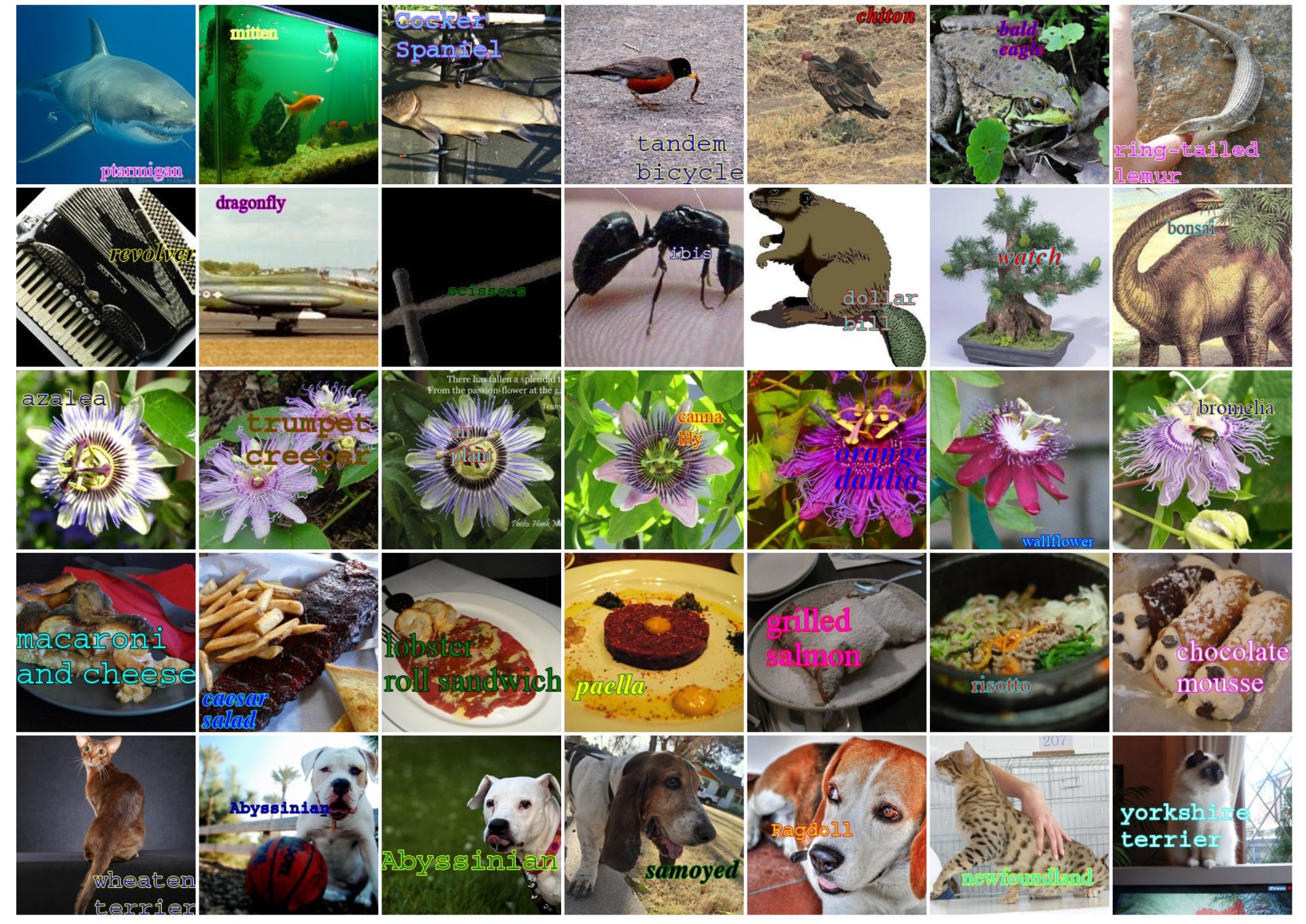

In this Sec., we will explain the details of the training data in Sec. 3.2 and test data in Sec. 4.2. When we train the DP vector (Sec. 3.2) and conduct experiments on classification (Sec. 4.2), we use synthetic typographic attack datasets. For training data, we add text to images from ImageNet-100 (Figure A). For test data, we add text to images from ten classification datasets (Figure B): ImageNet [7], Caltech101 [11], OxfordPets [33], StanfordCars [24], Flowers102 [32], Food101 [2], FGVCAircraft [29], DTD [4], SUN397 [46], EuroSAT [18]. To make typographic attack datasets, we followed the way of PAINT [19]. We resize the short dimension to 224 pixels using bicubic interpolation and crop 224 pixels by 224 pixels in the center, which is the standard CLIP [34] resize and crop augmentation. For fonts, we randomly choose from three fonts: Roman, Courier, Times. For font size, we randomly sample between 20 and 40 points. Also, we randomize over eight colors: red, green, blue, cyan, magenta, yellow, white, and black. We outline text with a 1-point shadow that is a different color from the main font color. The text is randomly placed in the image such that whole words are visible. Text is chosen from the class labels of the dataset except for the correct image labels.
For object detection, we also make synthetic typographic attack datasets using COCO [27] and LVIS [16] (Figure C). We use AdobeVFPrototype as a font. We randomize over eight colors: red, green, blue, cyan, magenta, yellow, white, and black. We outline text with a 1-point shadow that is a different color from the main font color. The text is randomly placed in each bounding box such that the whole words are visible. We adjust the font size so that the width of the text is less than 0.8 times the width of the bounding box.
Appendix C RTA-100


In Sec. 4.2, we use real-world typographic attack datasets. To increase the test data, we take pictures and make RTA-100, which is the biggest real-world typographic attack dataset (Figure D). We put tags that are labeled incorrect classes to objects. We choose the incorrect labels of the tags from the objects in our dataset. We take pictures from 10cm to 2m from the objects such that whole words are visible. For example, we write “pen” on the tag and put it on a frisbee. Then, we take a photo of the object. For fonts, we randomly choose from three fonts, as seen in Figure E. For the color of the tags, we randomly choose from 4 colors: yellow, green, blue, and pink. Also, we randomize over 4 colors for the color of the pen: black, red, purple, and brown. We randomly choose these elements in advance. The dataset contains 100 categories and 1000 images. We use iPhoneX’s camera, and the size of images is 3024 pixels by 3024 pixels. The code and dataset will be publicly available.
Appendix D PAINT
In Sec. 4.2, we compare our method with PAINT [19]. For training for PAINT, we train the model for 3 epochs (2400 iterations) with batch size 16 using learning rate 1e-5 with 200 warm-up steps with a cosine annealing learning rate schedule and the AdamW optimizer (weight decay 0.1), following the paper.
Appendix E Extended results on all datasets.
| Method | ImageNet | Caltech | Pets | Cars | Flowers | Food | Aircraft | DTD | SUN | SAT | Avg. |
|---|---|---|---|---|---|---|---|---|---|---|---|
| CLIP | 62.02 | 88.64 | 87.35 | 58.72 | 66.32 | 84.14 | 18.99 | 44.57 | 61.74 | 42.98 | 61.55 |
| Materzynska+ [31] | 54.38 | 80.53 | 75.01 | 40.33 | 51.86 | 55.01 | 13.23 | 36.28 | 51.06 | 37.32 | 49.50 |
| PAINT [19] | 61.82 | 88.48 | 85.23 | 55.30 | 64.73 | 80.51 | 17.73 | 42.61 | 61.69 | 38.20 | 59.63 |
| Ours | 62.48 | 89.28 | 87.22 | 57.47 | 63.82 | 83.65 | 19.26 | 40.64 | 61.41 | 43.85 | 60.91 |
| Method | ImageNet | Caltech | Pets | Cars | Flowers | Food | Aircraft | DTD | SUN | SAT | Avg. |
|---|---|---|---|---|---|---|---|---|---|---|---|
| CLIP | 39.10 | 63.97 | 58.95 | 21.02 | 31.32 | 56.27 | 10.83 | 25.53 | 34.02 | 4.86 | 34.59 |
| Materzynska+ [31] | 44.91 | 74.73 | 63.61 | 15.79 | 34.95 | 43.41 | 8.28 | 33.03 | 39.52 | 16.22 | 37.44 |
| PAINT [19] | 55.9 | 83.57 | 76.53 | 33.44 | 54.92 | 72.94 | 14.46 | 36.60 | 53.62 | 17.31 | 49.93 |
| Ours | 49.83 | 79.54 | 72.88 | 28.64 | 44.12 | 67.79 | 14.49 | 31.6 | 43.50 | 9.65 | 44.20 |
Appendix F Visualization
To visualize the changes in word information, we generate images conditioned on text prompts using VQGAN+CLIP [6]. Fig. F presents samples of generated images: the first row shows images generated with original VQGAN+CLIP, capturing the visual concepts of the prompt texts. In cases of “peas”, “corn”, and “flower”, the images show the words of the prompts. The images generated with VQGAN+CLIP+Ours can also capture the visual concepts and do not show prompt text; instead, they show nonsense strings. The experiment demonstrates words with DP lose little original meanings, ruining the text information.
