Quantum Mechanics Lecture Notes.
Selected Chapters
Abstract
These are extended lecture notes of the quantum mechanics course which I am teaching in the Weizmann Institute of Science physics program. They cover the topics listed below. The first four chapters are posted here. Their content is detailed on the next page. The other chapters are planned to be added in the coming months.
1. Motion in External Electromagnetic Field. Gauge Fields in Quantum Mechanics.
2. Quantum Mechanics of Electromagnetic Field
3. Photon-Matter Interactions
4. Quantization of the Schrödinger Field (The Second Quantization)
5. Open Systems. The Density Matrix
6. Adiabatic Theory. The Berry Phase. The Born - Oppenheimer Approximation
7. Mean Field Approaches for Many Body Systems - Fermions and Bosons
Chapter 1 Motion in External Electromagnetic Field. Gauge Fields in Quantum Mechanics
Electromagnetic potentials and appear in classical physics as auxiliary quantities which are introduced in order to simplify the form and solutions of the Maxwell equations, cf., Chapter 10 in Ref. [8]. The fact that they are not uniquely defined and can be changed without affecting any physical results by a transformation bearing a strange name of ”gauge” seems to be rather an annoying nuisance than a fundamental symmetry of nature.
This state of affairs undergoes drastic revision when quantum mechanical description is attempted. We do not know how to formulate such a description in the presence of the electromagnetic field without making an essential use of the electromagnetic potentials. Moreover the invariance under the gauge transformations becomes a profound symmetry of our world which lies at the origin of all known interactions. Because of this the fields which carry these interactions are termed gauge fields.
The problem of the quantum mechanical motion in an external electromagnetic field provides the simplest setup in which one encounters some of the strange and beautiful phenomena appearing as a result of the symbiosis of gauge fields and quantum mechanics.
Note. I have changed from CGS to SI units in Sections 1-8. The rest is in CGS.
1.1 Electromagnetic Potentials. The Hamiltonian
1.1.1 Electromagnetic potentials in classical physics
Let us begin by briefly recalling how the electromagnetic potentials are introduced. Classical electromagnetic field is described by two vector fields and . In the present chapter these fields will be considered as external, i.e. produced by sources (electric charges and currents) which dynamically are not a part of the physical system under consideration and are not effected by it. This means that the back reaction of the system on the sources of the field is negligible. Although in such circumstances E and B should be regarded as controlled externally by charge and current distributions and of the sources via
they can not be taken as completely arbitrary. Indeed irrespective of the configuration of and j these fields must satisfy the homogeneous pair of Maxwell equations
| (1.1) |
at every point in space and time. In order to have these equations automatically satisfied the familiar vector and scalar potentials and are introduced11 1 Although we use ”relativistic” notation for we use ”non relativistic” terminology and call it a scalar potential. This is done by noticing that the first of the equations above means that B must be a curl of a vector field . Using this in the second equation gives
restricting the combination to be a gradient of a scalar field. One has therefore
| E | |||||
| B | (1.2) |
Unlike the field strengths E and B, the electromagnetic potentials can be regarded as unrestricted so that any and can be realised by the poper choice of the external charge and current distributions.
The use of the electromagnetic potentials however presents another problem. They are not unique since the gauge transformation
| (1.3) |
with an arbitrary function leaves E and B invariant. As was already mentioned above this invariance, called the gauge invariance, has profound consequences in quantum mechanical systems and will be discussed at length below. At the moment we just notice that because of it only three among the four functions A and are independent. In general one combination of the four functions can be eliminated by a suitably chosen gauge transformation. For instance choosing
(with arbitrary ) eliminates and leaves as the only independent degrees of freedom of the electromagnetic field.
1.1.2 Classical Hamiltonian and equations of motion
Classical non relativistic equation of motion for a particle with electric charge and mass in a given electromagnetic field is obtained by using the Lorenz force in the Newton law
| (1.4) |
In order to obtain the quantum mechanical description one can follow either the canonical or the path integral quantization procedures. We will start with the former. We first determine the classical canonical variables and the classical Hamiltonian function of the problem.
The above equation is in terms of coordinates and velocities so it is is most convenient to start by determining the Lagrangian of the system. This is
| (1.5) |
Indeed have
and
In components
So have
which is the Newton equation (1.4). Indeed recalling Eq.(1.2) one sees that the fist term is , while the last term can be transformed as
where we used the antisymmetric symbol 11 1 The Levi–Civita symbol is defined by and the antisymmetry property under interchange of any indices, etc. does not change under cyclic permutations . . to write vector products, e.g
These two equalities are related by a useful identity
The above calculations show that the canonical momentum is
| (1.6) |
which expresses perhaps the most unusual aspect of the motion in the EM field - the fact that . In the literature one often meets the term ”kinetic momentum” referring to the familiar .
Expressing and using
with the above we find the Hamiltonian function
| (1.7) |
It is not difficult (and not surprising) to show that with this the equation of motion (1.4) is equivalent to the two Hamilton equations
1.2 Quantization
1.2.1 The orbital part
Having established the form of H we follow the canonical quantization procedure and consider the Schrödinger equation with the Hamiltonian operator which is obtained by replacing r and p in by the operators and ,
| (1.8) |
1.2.2 The spin magnetic moment
Experimental evidence shows that this Hamiltonian is capable of describing only particles which do not carry spin. It must be modified when the spin degrees of freedom are present. This should not be too surprising since already in classical physics the energy of a spinning charged particle receives an additional contribution apart from the orbital motion. This contribution arises from the interaction with the magnetic field B of a localized distribution of electric current which a spinning charge creates. For a ”point like” particle, i.e. a particle the size of which is much smaller than the scale over which changes, the corresponding energy is
where is the magnetic moment of the current, cf., Chapter 5 of the Ref. [8],
For composite particles the total current is a sum over internal components
each with its dynamics so the calculation of is in general not an easy task. However if all the components have an equal charge to mass ratio the magnetic moment can be written as
| (1.9) |
Experimental data as well as theoretical considerations (cf., Section 1.8 below) indicate that for elementary particles like electrons this classical linear relation between and the angular momentum of a system holds also between the corresponding quantum mechanical operators of the magnetic moment and the spin . However the proportionality coefficient in general does not coincide with the classical value. To emphasize this difference it is conventional (for charged particles) to write the relation between the operators and s as
| (1.10) |
with - the particle charge and - dimensionless coefficient called the gyromagnetic factor or for short the g-factor. Theoretical methods which allow to determine and examples of their applications are considered in Section 1.8.
1.2.3 The Schrödinger equaion
Adding the term to the Hamiltonian operator (1.8) one can write the Hamiltonian for an elementary particle with a spin in an external EM field as
| (1.11) |
and the corresponding Schrödinger equation
| (1.12) |
where
is a function of space and spin variables r and .
In writing out the square in this equation one should not forget that the operator in general does not commute with the vector A which is a function of coordinates. Since , one can write
The operators and A commute if . This happens e.g., for which is a possible choice of A in a particular case of a uniform magnetic field22 2 Verifying (1.13) .
In the following sections we will examine various properties of the equation (1.12) and will present its solutions for some particular simple choices of the electric and magnetic fields.
1.3 Gauge Invariance
1.3.1 Gauge transformations in quantum mechanics
The electromagnetic field enters the classical and quantum equations (1.4) and (1.12) via very different sets of variables. The classical equation depends on the physically measurable variables E and B of the field whereas in the Schrödinger equation the field enters via non uniquely defined and seemingly auxiliary objects A and . This is not an accident. At present no formulation of quantum mechanics exists which does not explicitly use the electromagnetic potentials. Schrödinger and Heisenberg pictures require the Hamiltonian while the path integral quantization uses the Lagrangian (cf., below, Section 1.10) and both objects can not be written without A and . Since the potentials are not uniquely defined and can be changed by a gauge transformation one must address the question of how unambiguous physical results are obtained in such a situation.
Unlike in classical mechanics where gauge transformations do not change the equations of motion the Schrödinger equation (1.12) and therefore also its solutions are transformed in a non trivial way33 3 In this and many of the following sections the dependence of on the spin variable will not be of interest and will be suppressed for brevity. . It is not difficult to find how the transformation of is related to the transformation of the potentials. For this we notice that A and enter the equation only in the combinations
Thus if is a solution for a particular choice of A and then
| (1.14) |
satisfies
| (1.15) |
and therefore solves the Schrödinger equation for the transformed potentials (1.3) (please note the primed and on the right hand side of the expressions above).
We see that the classical concept of the gauge transformation undergoes a generalization in quantum mechanics. Now not only the potentials which describe the electromagnetic field but also the wave functions describing the material particles must change simultaneously according to the rules (1.3) and (1.14). This change is local, i.e. it is different for different points in space and time. One often emphasizes this aspect by calling the transformation given by Eqs. (1.3), (1.14) a local gauge transformation to distinguish it from a global transformation in which the wave function is multiplied by a constant phase factor.
It is seen that the combinations and defined in (1.15) transform under a local gauge transformation in a particularly simple way – i.e. as if it were a global transformation. These combinations are called gauge covariant derivatives in theories with gauge fields. The way to introduce the electromagnetic field in the dynamical equations by replacing the ordinary derivatives and by the gauge covariant combinations is known as minimal coupling.
1.3.2 Gauge symmetry vs gauge invariance
We may now ask a question as to whether the classical gauge invariance also holds in quantum mechanics, namely whether the result of any measurement is invariant under gauge transformations which now include also the local transformation (1.14) of the wave function. It is an empirical fact that the answer to this question is positive. Moreover it is also clear that this invariance known as the local gauge invariance is a profound fundamental symmetry of the quantum mechanical description in the presence of gauge fields.
It is important to note that this symmetry does not mean that the wave functions must be invariant. Like with other fundamental symmetries, e.g. the invariance with respect to translations and rotations, the gauge symmetry means that the wave functions transform in a particular way given by Eq. (1.14), i.e they form a representation of the corresponding group of transformations.
Here, however, the similarity ends. Unlike other symmetries the gauge symmetry demands that the observable quantities must not be effected by the gauge transformations and therefore must be ”gauge scalars”, i.e. depend on gauge invariant combinations of and . No ”gauge vectors”, ”gauge tensors”, etc, are ever observed. The origin of this difference can only be understood when the full quantum dynamics of the electromagnetic field and its coupling to matter are discussed.
We conclude this section by noting that explicit appearance of the electromagnetic potentials in the equations of quantum mechanics makes the gauge invariance a very subtle symmetry. Its consequences and generalizations are important aspects of the modern physics. We will make a special point in this chapter to illustrate some of the related physical ideas and results.
1.3.3 The Gauge Principle – symmetry dictates
interactions
In the previous section we started with the known transformation properties of the potentials and then on the basis of the special manner in which they entered the Schrödinger equations – i.e. in combinations and , – derived the required transformation properties of the wave functions which were necessary in order to keep the Schrödinger equation form-invariant.
Imagine now that we reverse this derivation in the following manner. Let us begin by considering the free Schrödinger equation
This equation is obviously invariant under the global gauge transformations i.e. the transformations (1.14) with a constant independent of (r,t). This global gauge invariance is a fundamental feature of the Schrödinger equation. One of its notable consequences is the conservation of the integral . This integral is the total probability or, when multiplied by , the total electric charge. The relation of its conservation to the global gauge invariance is not intuitively obvious but can be rigorously derived by the applications of arguments of the Noether theorem to the Schrödinger field.
Now let us see what happens if one demands that the nature should be invariant not only under the global but also under local gauge transformations, i.e. with the (r,t)-dependent phase in Eq. (1.14). It is obvious that the free Schrödinger equation will not satisfy this demand since its derivatives will act on the local phase producing additional terms with and . With the hindsight of the previous section we can however write a more general Schrödinger equation which will be locally gauge invariant.
In order to compensate for the derivatives and and eliminate them from the transformed Schrödinger equation we must
(a) ”postulate” the existence of a field described by the potentials A and ,
(b) replace the ordinary derivatives and in the equation by the gauge covariant combinations , and
(c) require that the potentials transform according to Eq. (1.3) simultaneously with the transformation (1.14) of the wave functions.
The demand of the local gauge invariance is thus turned into a powerful heuristic principle – The Gauge Principle, which, had we not known about the electromagnetic field, led us to ”discover” its existence and the way it must appear in the Schrödinger equation.
Of course the last, spin-dependent term in (1.12) would not be deduced in such a procedure and should be justified separately. The need for this separate discussion of the spin interaction with the electromagnetic field disappears when a fully relativistic theory of elementary particles is considered, cf. Section 8.1 in Ref. [2] or Chapter 3 in Ref. [3]. Moreover it can be shown that the entire Maxwell electrodynamics is fully consistent with the The Gauge Principle supplemented by very general requirements of the time-space translational invariance and the Lorenz invariance.
It also turns out that the fields responsible for all other known interactions, i.e. weak, strong and gravitational are consistent with The Gauge Principle in a similar way. Namely for every known interaction there exist a a global symmetry of a non interacting theory which becomes a local symmetry after the interaction is introduced. The potentials describing the interaction are the compensating gauge potentials which are necessary to introduce in order to satisfy this demand are the fields of the fundamental interactions. Thus The Gauge Principle essentially means that Symmetry Dictates Interactions. The Gauge Principle for general relativity for example means that the theory is invariant under local Lorenz transformations. In Section 1.12 below we consider an example of how a so called non abelian gauge field appears as a result of the demand that the Schrödinger equation is invariant under local non abelian transformations.
1.4 Electric Current Density.
1.4.1 The orbital part
Let us derive the quantum mechanical expression for the current density of charged particles. We will start by considering the continuity equation for the charge density . Multiplying the Schrödinger equation (1.12) on the left by and its complex conjugate by and subtracting one obtains in a standard way that with the current density
| (1.16) |
This expression is the expectation value of the operator
| (1.17) |
of the current density due to orbital motion with the velocity
This operator is just what is obtained from the classical expression for a point particle by replacing the classical quantities and with the corresponding operators and and symmetrizing the final expression in order to make it hermitian.
1.4.2 The spin contribution
The missing feature in the above expression for the current is the absence of the contribution from the spin of the particle. This is the reason we have added to it the index . As we have already discussed a spinning charged particle creates a local distribution of electric current at its location and one should expect to find an appropriate term in the current density in addition to the contribution of the orbital motion. We have missed this term because as we will see in a moment it is in the form of a rotor of a vector (a so called solenoidal term) and therefore can not be seen in the continuity equation which depends only upon the divergence of the current.
In order to correct our result let us consider a physical system of charges placed in positions and put it under the influence of an external electric field . We start classically and consider a time interval during which these charges move distances . As a result their total energy is changed by
The expression in the square brackets here is the total current density flowing in the system, so that
| (1.18) |
We assume that this relation holds also for quantum mechanical expectation values. Considering for simplicity one particle and let us form the expectation value of the Hamiltonian (1.11)
| (1.19) | |||||
We also have
| (1.20) |
This relation (sometimes called the Feynman–Hellmann theorem) is valid since the term vanishes on account of the Schrödinger equation .
In order to find the time derivative of the Hamiltonian we note that it depends on time only via the time dependence of the potentials . Part of this time dependence is not physical and is related to the time dependent gauge transformations of A and . In order to avoid this fake time dependence we fix the gauge by choosing . This choice does not fix the potentials completely but the only freedom left is time independent gauge transformations, i.e. Eq.(1.3) with time independent . With this choice we have that
| (1.21) |
Using (1.2) with and Eq. (1.18) we obtain the general relation for the electric current
| (1.22) |
Varying H with respect to A and using we obtain
| (1.23) | |||||
Integrating by parts in the first term, using the identity
for the last term in this expression and assuming that the surface terms vanish we obtain the following expression for the current
| (1.24) |
The first two terms are just the ”orbital” current already obtained earlier from the continuity equation. The last, ”solenoidal” term is the spin contribution which has the appearance of the classical relation between the current and the magnetic moment
1.4.3 Convective, diamagnetic and spin parts of the current
The first term in the expression (1.24) for the current is called the convection current and coincides with the usual expression for the current density in the absence of the electromagnetic field. It is not gauge invariant without the second term which is called the diamagnetic current. The third, spin term in is obviously gauge invariant by itself.
In elementary quantum mechanics one develops certain intuition about currents associated with given wave functions. In particular one is used to the fact that non vanishing current density does not appear if the wave function is real, that the current is related to the local complex phase of , etc. This intuition is founded entirely on the first term in Eq. (1.24) and could be misleading in the presence of electromagnetic field. In this case one finds for instance a non vanishing orbital current density
for a real wave function. Of course the freedom of local gauge transformations (1.14) makes the phase of and the difference between real and complex wave functions into something which depends on the choice the gauge and therefore unphysical.
1.5 Motion in a Uniform Electric Field
Already such a simple problem as the motion of a charged particle in a constant uniform electric field E exhibits peculiarities of gauge fields in quantum mechanics. Classically everything is simple. The particle moves with the constant acceleration in the direction of the field and has a constant, determined by initial conditions velocity perpendicular to this direction. In quantum mechanics one may have differently looking descriptions depending on which of the many (i.e. continuous number of) possible choices of A and is made leading to the same constant E and . Of course the gauge invariance will assure that all physical quantities are independent of the gauge choice but in actual calculations it may require some efforts to see the connections.
1.5.1 Static gauge
We will explore in some detail two gauge choices, the simplest and most familiar gauge , and another, time-dependent gauge , In the former case the time and the coordinate variables are separable in the Schrödinger equation
| (1.25) |
and moreover also separable are the coordinates parallel and perpendicular to Choosing the axis parallel to E and denoting by subscript vectors which are perpendicular to E one can write the stationary solution as
| (1.26) |
where and are the eigenenergies and the corresponding eigenfunctions of the motion parallel to x. They satisfy the one dimensional Schrödinger equation
| (1.27) |
where we denoted .
In the equation for the behavior of the potential at infinite values of x is such that the energy levels form a continuous spectrum of values from to . They should correspond to motion which is bounded from but unbounded in the direction . The wave functions must vanish in the region of large and negative x and therefore the energy levels are non degenerate. Indeed if there were two solutions and for the same then
| (1.28) |
so that the Wronskian . The condition that wave functions vanish at means that leading to i.e. the two solutions would in fact coincide.
1.5.2 Linear potential - the Airy function
The simplest way to solve the equation for is to consider it in the momentum representation. Inserting the expansion
| (1.29) |
in the equation for we easily obtain
| (1.30) |
Integrating this first order equation we find
| (1.31) |
The constant in front of this expression must be determined by normalization. Choosing e.g., to normalize on the delta function in
| (1.32) |
we obtain . The wave functions in the position representation are
| (1.33) |
where we denoted and introduced the notation
| (1.34) |
The function defined by this integral is called the Airy function. We will explore some of its properties below, cf., also Ref. [10]. The graph of the Airy function is shown in Fig. 1.1.

It is instructive to explore the asymptotic behavior of the wave function for . This can be found by using the saddle point approximation
cf., https://atmos.washington.edu/ breth/classes/AM568/lect/lect22.pdf
in order to evaluate the integral in (1.33). Differentiating the exponent in the integrand we obtain that the stationary value of p must satisfy
| (1.35) |
This is the classical – energy momentum relation in the potential . It is an example of a typical ”cleverness” of the saddle point method – when a phase of a rapidly oscillating integral depends on external physical parameters (the coordinate x in (1.33)) the saddle point condition frequently has a transparent physically significance. The difference with the classical physics is that does not have to be real. Only for , i.e. in the region where the classical motion is allowed, is real, but it is pure imaginary in the classically forbidden region . In both cases there are two solutions corresponding to the two signs in the square root
| (1.36) |
According to the rules of the saddle point approximation both saddle point solutions should be retained in the real case while only the saddle point with decaying exponential should be admitted in the imaginary case. We thus find for (1.33)
| (1.37) |
We will see in the section devoted to the semiclassical limit that these expressions correspond to the semiclassical approximation for wave functions. As required the wave function decays exponentially in the classically forbidden region . In the classically allowed region the positive and negative momenta with equal amplitudes coexist for a stationary quantum mechanical state producing the interference cosine with the argument which can be written as
| (1.38) |
in terms of the classical action . The classical momentum determines the local wave length which decreases with increasing x in accordance with the uniform classical acceleration in the direction of the field and the de Broglie relation.
1.5.3 Time dependent gauge
Let us now examine how this problem looks in another gauge , . We use the gauge transformation (1.14) with in the equation (1.25) and obtain
| (1.39) | |||||
where we denoted by the transformed wave function.
A simple solution of this equation is a plane wave and we obtain for
| (1.40) |
with the time dependent amplitude satisfying
| (1.41) |
Integrating we find
| (1.42) |
where is an arbitrary constant, and we used the same notation for and as in the previous section.
We note that with this solution the wave function before the gauge transformation (1.39) is
| (1.43) |
which of course is a solution of the Schrödinger equation (1.25) in the static gauge. The set of these time dependent solutions with different k’s is identical to the set (1.26) of stationary solutions as far as the motion in is concerned. However in the direction of the field the sets look quite different and the point to note here is that in different gauges the same problem may have a very different appearance.
Of course mathematically both sets are equivalent and one can easily show that each can be expressed as a linear combination of the other. The time dependent solution is closer to the classical intuition of the accelerated motion under a constant force.
It is instructive in this simple problem to compare the calculations of the currents for two solutions , Eq. (1.43), and the corresponding transformed one , Eq. (1.40). One will get different results with the two solutions
for the convective part of the current given by the fist part of Eq.(1.24). But this difference is ”counterbalanced” by the different second diamagnetic term in the current expression. It is zero in the static gauge but is
in the time dependent gauge. The end results is of course the same expression as it must be for the gauge invariant quantity.
1.5.4 Translations in uniform E. Symmetries in the presence of gauge fields
Physics in a constant electric field must be invariant under translations of coordinates with a constant vector . Applying this transformation in the Schrödinger equation (1.25) one at first finds that it is not invariant – the term is added to the Hamiltonian. This term however can be removed if one simultaneously performs a gauge transformation of the wave function
| (1.44) |
The Schrödinger equation is invariant under this combined transformation which must be therefore adopted as the definition of the translation in the present case. One can call it ”electric translation” in analogy with the modified ”magnetic translations” in a uniform magnetic field, cf. Section 1.6.3 below.
This feature of modification of the standard symmetry transformations by additional gauge transformations is quite typical for theories with gauge fields. It accounts for the fact that changing the coordinate system may also effect the gauge choice and care must be taken to return to the original gauge. The generator of the infinitesimal translations in the expression above is obviously
| (1.45) |
The symmetry means that it must be conserved and indeed one finds that
with as it appears in the right hand side of (1.25).
1.6 Motion in a Uniform Magnetic Field
We will now consider the quantum mechanical motion of a charged particle in a uniform external magnetic field B which is constant in magnitude and direction over the entire space. For convenience we present the discussion for electrons, i.e. we take the value of the charge
1.6.1 Classical motion. The guiding centers
It is instructive to recall first the classical solutions of the problem. The classical equation of motion is
Let us choose the direction of the axis parallel to B. Then the motion along is free,
with constant and determined by initial conditions.
The equations for the and components are
| (1.46) |
An important observation to be made here is that these Newton equations for the velocities of motion in a plane perpendicular to B have the same formal appearance as the Hamilton equations of a one dimensional oscillator with and formally proportional to the respective coordinate and momentum of the oscillator. The solution of these equations is ”harmonic motion” in the ”velocity space” with the frequency
called the cyclotron frequency and
| (1.47) |
so that the trajectory in the (x,y) plane is
| (1.48) |
Here and are constants of the motion the values of which are fixed by the initial conditions at some initial time .
The physical meaning of these constants is the following. The above solution describes a circle with the radius . The position of the centre of the circle is given by the coordinates and which are therefore conventionally called the coordinates of the guiding center, cf., Fig. 1.2 below. The value of also determines the energy
of the motion in the plane44 4 The conservation of this quantity is trivially ”discovered” by multiplying the two equations (1.6.1) respectively by and and adding. This energy is independent of where on the plane the orbit is situated, i.e. is independent of the values of and .
Using the terminology of quantum mechanics we can say that the above circular motion is degenerate - all circles with the same radius have the same energy. This degeneracy is characterized by different values of the guiding centre coordinates and so one can say that the classical motion is degenerate. As we will see in the next section in quantum mechanics the motion is ”only” degenerate. It is important to observe that the expressions of the guiding centre coordinates as given by resolving (1.6.1)
| (1.49) |
are constants of the motion
This fact, which is trivial in classical mechanics will play a very important role in the quantum mechanical treatment of the problem.
1.6.2 Landau levels
The quantum mechanics of this problem was first worked out by Landau and the corresponding solution is known as Landau levels.
The eigenenergies
The quantum Hamiltonian of a particle without spin in this case is
| (1.50) |
where the vector potential must be chosen such that is a constant vector parallel to . With simple choices of A it is possible to find explicit solutions of the corresponding Schrödinger equation as we will discuss in detail below. At the moment however we prefer to proceed in a more general manner and show that many features of the solution can be anticipated on the basis of simple considerations which are useful to follow in order to gain a better understanding of the physics of the problem.
We start by considering the commutators of the components
of the velocity operators which enter the Hamiltonian (1.50). They are easily calculated,
| (1.51) |
These non vanishing commutators show that for a general magnetic field one can not have definite values simultaneously for all 3 components of the velocity.
In our particular case of a constant B along the axis only the commutator is not zero. This means that commutes with , Eq. (1.50). Since moreover one can choose and and to be functions of only one has
so that the parts of depending on and on are separable. The –dependent part of the wave function must be a plane wave with describing quantum free motion in accordance with the classical case.
The part of describing the motion in the plane,
| (1.52) |
is proportional to the sum of squares of the operators and with a constant commutator
This suggests to define rescaled variables
with the canonical commutator
in terms of which the operator takes the form
of the Hamiltonian of a one dimensional oscillator with mass and frequency in accordance with the character of the corresponding classical motion. The spectrum of the oscillator is well known and adding it to the free motion eigenvalues of the term we obtain the eigenvalues of as
| (1.53) |
We have succeeded to obtain the eigenvalues of the Hamiltonian (1.50) on the basis of the commutation relations without solving the Schrödinger equation. There however remains a problem. The eigenvalues depend only on two quantum numbers and whereas dealing with three degrees of freedom one must find three quantum numbers which characterise the eigenfunctions of .
Degeneracy of the Landau levels. Quantum guiding centers
The independence of on the third quantum number means that the energy levels of the problem are degenerate and we will presently determine the reason and the nature of this degeneracy. For this purpose let us consider the quantum mechanical operators corresponding to the guiding center coordinates, Eq. (1.49),
| (1.54) |
We easily find that they both commute with all the components of the velocity operators,
| (1.55) |
Indeed, e.g.
Therefore and commute with , i.e. are conserved as in the classical case. As in the classical treatment the energy of the motion is independent of these quantities. However we find that their commutator is not zero. Indeed using (1.55)
| (1.56) |
This relation is commonly written as
| (1.57) |
where the constant
is called the magnetic length.
The non vanishing commutator between and means that they can not both have simultaneously definite values and moreover the constant value of the commutator shows that like the velocity operators above, their properties are similar to a canonical coordinate–momentum pair. Only one of the two can be specified and since it is conserved its eigenvalues should provide the missing quantum number which we are looking for in order to characterize the degenerate eigenfunctions belonging to the same eigenenergy . In fact the existence of the pair of non commuting conserved operators is the cause of the degeneracy of . If we choose the states of the system to be eigenfunctions of, say, operator, acting on one of them with will produce a different state with the same energy. As we will show below there is a deep relation between the properties of the operators and and the basic symmetry of the system – the translational invariance.
The eigenfunctions
From the commutation relations Eq. (1.57) it follows that for the eigenstates with definite the values of are completely undetermined so that the position of the center of the quantized cyclotron orbit will have equal probability to be found at any point along the line with the given . To see this explicitly we now turn to the solutions of the Schrödinger equation which have definite values of . We need to choose first the gauge for the vector potential A. The explicit forms of ,
and of
suggest the following convenient choice
| (1.58) |
for which
and the Hamiltonian
| (1.59) |
The eigenfunctions of and have the form
| (1.60) |
with yet undetermined . For convenience we have assumed that the motion in the and the directions is limited by large but finite intervals and with periodic boundary conditions.
Inserting in the Schrödinger equation and separating the variables we obtain
| (1.61) |
where we denoted . This is the equation of a harmonic oscillator centered around the eigennvalue of . As anticipated the eigenenergies are given by (1.53) and are independent of . The eigenfunctions are
| (1.62) |
where are the normalized eigenfunctions of harmonic oscillator
| (1.63) |
with – the Hermite polynomials. The first few functions are
| (1.64) | |||||
Imposing periodic boundary conditions in the direction we find that in Eq.(1.60) takes discrete values separated by distances . We thus have one state per area in the x-y plane. The dependence of the wave functions on y via the plane wave phase means that the probability to find a particle is independent of this coordinate. It also seems to suggest that like in the - direction there is a free motion also in the y-direction. This however is not corrects as it is based on the experience in situations in which there was no gauge field present. In this case the wavefunction’s phase is gauge dependent so to evaluate what motions it describes one must form gauge invariant observables. We will do this below by calculating the current density components with physically interesting results.
In the direction the state is centered around the value . Its extension can be determined, using e.g., the equipartition property of the oscillator meaning that the average potential energy is one half of the total energy, . This gives . Each degenerate energy level can thus pictorially be viewed as a two dimensional plane filled with overlapping (for ) ”strips” occupied by individual quantum states parallel to the y axis representing quantized cyclotron orbits uniformly ”smeared” along every strip. This picture repeats itself for every n and with the radius of the orbits, i.e. the thickness of the strips growing as . The smearing of the orbits is the result of the Heisenberg–like uncertainty relation between the guiding center coordinates and .
The degenerate energy levels which we have just described are called Landau levels. Choosing to have defined values will lead to the same picture of Landau levels but with the strips parallel to the x axis. It is amusing to consider what happens if more complicated functions of and are chosen to have defined values. Suppose we fix . Then the strips in the picture above will have the shape of concentric circles around the origin. Choosing fixed with some constants a and b will lead to strips of elliptic shapes, while fixing the function (symmetrized to make the corresponding operator hermitian) will result in a hyperbolic shape of the strips, etc.
In Fig.1.2 we illustrate some of these cases. Of course all the choices above are equivalent as long as the degeneracy remains but some may be singled out if a perturbation removing this degeneracy is added to the Hamiltonian.

When choosing the eigenvalues of the operator instead of for the characterization of the degenerate wave functions it should be more convenient to choose the gauge , in which is just . For a combination the symmetric choice , , is the most appropriate. In the literature it may sometimes seem that the choice of the gauge determines which combination of and will be diagonal. Our remark here is meant to clarify the correct order of choices .
The square of the magnetic length appearing in the commutator of the guiding center coordinates plays the role of the ”Planck constant” for these variables. Therefore the analogue of uncertainty relation must hold. We also recall from the statistical physics that in the semiclassical picture quantum states ”occupy” phase space volume . Here we may expect an analogous situation that a single state of a degenerate Landau level ”occupies” an area in the plane of which is . And indeed we have seen this in the particular case of the solutions (1.60). The physical meaning of this minimal area is simple and profound – the magnetic flux through this area is ratio of universal world constants
Such magnetic flux has a special notation
| (1.65) |
and a special name - magnetic flux quantum. We will meet this quantity a number of times in these notes (cf., below). Let us stress that its name doesn’t mean that the magnetic flux in such problems is quantized. Rather, as we see here and will be seen below certain physical features get repeated with as a period.
As can be seen from the above discussion the density of single states in a degenerate Landau level is the inverse of which is independent of n and of the way we choose to classify the degeneracy. The mnemonic rule of ”one state per one flux quantum” is something which is encountered in many quantum mechanical problems in the presence of magnetic field and is therefore well worth remembering.
Currents and edge currents
Individual states in a Landau level carry a non vanishing current density. Apart from an obvious contribution from the free motion in the z–direction one also finds current distribution in the x-y plane. Qualitatively one expects that in this plane the quantum mechanically smeared cyclotron orbits with one fixed guiding center coordinate should combine to give opposite currents parallel to and concentrated on the edges of the strip occupied by the state and have zero current on the midline of the strip.
We easily find for the states Eq. (1.60) using Eq. (1.24) for the current
| (1.66) |
where we denoted the particle density
The appearance of the lengths and is related to the (standard) normalization of the wavefunction (1.60) to one particle.
The wave function as given by any of the solutions Eq. (1.62) is concentrated in a symmetric strip around which means that the current density has an antisymmetric profile with respect to . Because of this antisymmetry the total current
| (1.67) |
flowing in the y-directions, i.e. along the state in the x-y plane is zero for these states.
If one adds a constant electric field parallel to the –axis one can still find exact wave functions (cf., homework problems or tutorial). The current density profile of these wave functions will change from antisymmetric to asymmetric and the total current in the direction will not be zero.
Another interesting non zero current carrying Landau states appear at the edges of the x-y plane. Let us assume that an additional potential with the shape shown in Fig. 1.3 is added to the Eq. (1.61)
| (1.68) |
This potential simulates the edges of the sample in the x direction.
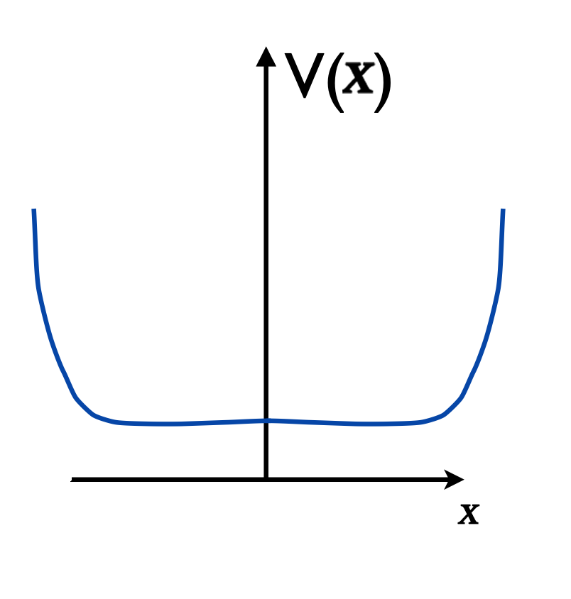
It is instructive to examine how the combined potential
changes when plotted for different guiding center coordinate values relative to the positions of the potential walls representing the edges. The shape of getting more narrow for the values of near and ”inside” the edges indicates that eigenenergies will break the degeneracy of the Landau levels in such a way that they become rising functions for such values of . Recalling the width which the unperturbed Landau levels occupy we can approximate for low values and the potential slowly varying on the magnetic length scale as
| (1.69) |
In this approximation the modified Landau levels similar to the unperturbed ones form an ”equidistant ladder” with each step having the shape of .
The asymmetric shape of the combined for near the edges means that the resulting eigenfunctions will not depend on via as in Eq. (1.62) and will not have the harmonic oscillator symmetry around as in the unperturbed Landau states. This in turn means that the current density along the edge will not have an antisymmetric profile with respect to and therefore the total current flowing in the x-y plane for such states near the edges will not be zero. Such currents are called ”edge currents”. They correspond to the skipping classical orbits near potential walls, move in opposite directions on the opposite edges and play important role in explaining the Quantum Hall Effect, cf., Ref. [13].
Let us express the energy of a given state using
with denoting the Hamiltonian operator in the left hand side of Eq. (1.68). Using the Feynman-Hellman theorem55 5 The theorem relates the derivative of the eigenenergy with respect to a parameter to the expectation value of the derivative of the Hamiltonian with respect to that parameter. The proof is straightforward where it was used that one obtains
| (1.70) |
Comparing with the expression for the current density in Eq. (1.66) and ignoring for convenience the direction we find the relation
| (1.71) |
where is the total current of a single particle in the state. Referring to Eq. (1.69) with as shown in Fig. 1.3 one sees clearly where the edge currents are expected, their magnitude and direction.
1.6.3 Degeneracy of Landau levels and space symmetries
Conservation laws are always results of symmetries and the existence of the conserved operators , and is not an exception. They are related to the basic symmetry of the motion in a uniform field – invariance under translations. This invariance is however not explicit in the Hamiltonian (1.50) which changes under the translation r to with an arbitrary constant vector a. We have already encountered a similar phenomenon in the simpler case of a uniform electric field. Also here the the Hamiltonian (1.50) remains invariant if simultaneously with the proper translation one performs a suitably chosen gauge transformation. The conserved quantities should be the appropriate generators of these combined transformations.
To see this in detail we observe that after a proper translation the Schrödinger equation with the Hamiltonian (1.50) has the same form but with the different vector potential . For a constant B however the difference is a gauge transformation, i.e. it is a gradient of a scalar function. It will be sufficient to show this for an infinitesimal a for which we have . The last term is
and for a constant B it is indeed a gradient
| (1.72) |
It can be removed from by a gauge transformation of the wave function in addition to the proper translation. The symmetry transformation is therefore
| (1.73) |
where we have used the proper translation operator for infinitesimal a to write in terms of .
The combined transformation (1.73) is what should be called translation in the presence of a magnetic field (the term ”magnetic translation” is sometimes used). The generators of this transformation are read off the linear term in found after multiplying the brackets in Eq.(1.73). They are
| (1.74) |
For translations along the z axis this is just whereas for the translations along the x and y axes we obtain respectively and in terms of the operators of the guiding center coordinates.
It should now become intuitively clear why these operators do not commute. We expect that the result of translating the wave function parallel to x and then parallel to y should not be the same as translating it in the opposite order. The difference should be related to the Aharonov-Bohm phase (see Section 1.7 below for its definition) induced by the flux of the magnetic field through the rectangle obtained in the course of these reversed order translations. Let us see how it happens. Transporting a wave function by an infinitesimal followed by and then by and respectively one indeed obtains keeping the terms up to a 2nd order in the translations and
| (1.75) |
where we denoted by and the corresponding vector components of the operator of translations (1.74) and – is the flux through the rectangle. Since the first non vanishing term in the expression above apart of unity was quadratic and proportional to it was necessary to keep the quadratic terms in the operators of each translation.
A similar discussion concerning the generalization of transformations and their generators can be worked out for another symmetry of the problems – the rotational symmetry around the direction of the magnetic field B. We will leave this for homework or tutorials.
1.7 The Aharonov - Bohm Effect
1.7.1 Local and non local gauge invariant quantities
We have emphasized in Section 1.3.3 that all observable quantities in a theory with a gauge field are gauge invariant. Perhaps the simplest such quantities are the electric and magnetic fields and the particle density . In the expression for the electric current density considered in the previous section we encountered another set involving the derivatives of – the combinations to which we can also add their time dependent partner . These combinations are gauge invariant due to the simple transformation properties of the gauge covariant derivatives (1.15).
A distinct feature of all these invariants is that they depend on and and their first derivatives at the same space–time point, i.e. they are local. Consider however a circulation integral taken around some closed contour drawn in space. By the Stockes theorem this integral is equal to the flux of B through the contour and is therefore gauge invariant. This is an example of a non local gauge invariant quantity. In the following sections we will discuss situations in which the non trivial dependence on leads to unexpected quantum mechanical effects which are collectively known as the Aharonov–Bohm effect, Ref. [6]. The sensitivity of the quantum theory to non local gauge invariants can be traced to essential non locality of the quantum mechanical description — eigenvalues and expectation values of various physical quantities such as energy, angular momentum, etc., depend on what happens with the wave function in the entire configuration space of the system.
Concluding this section we mention that in addition to the circulation of the vector potential another type of non local gauge invariants appears in certain physical applications. These are bi-local quantities of the type
Under gauge transformations the exponential and the wave functions produce phase factors which cancel each other. Quantities like this are often met in the field theoretical context and recently in certain many body problems.
1.7.2 Quantum mechanics ”feels” non zero even if on and near the contour C
Let us consider a region of space in which local invariant quantities E and B are zero but in which contours can be found for which does not vanish. A simple example is a region outside of a long thin tube with impenetrable walls and a non zero magnetic field concentrated inside and running parallel to the tube, Fig.1.4

Non zero circulation integrals are obtained for the integration contours which wind around the tube. Since by assumption outside the tube the details of a particular contour are of no importance except for the number of times it winds around the tube and the direction of this winding. Denoting this number by one can write
| (1.76) |
Here denotes the magnitude of the total flux of the magnetic field in the tube. The circulation integrals outside the tube depend only on and not to the details of the magnetic field distribution. One conventionally refers to such a tube as a solenoid and to such an isolated magnetic flux as the Aharonov–Bohm flux (AB flux for brevity).
1.7.3 ”Gauging out” the AB flux. Periodic dependence on its value
Classically the free motion of a particle in the outside region is not influenced by the presence of the field inside the tube. At first sight one may reach a similar conclusion in the quantum mechanical description. Indeed to write the Schrödinger equation one needs to determine first the electromagnetic potentials. Since in the outside region one must have that A must be a gradient of some scalar,
| (1.77) |
With such A (and ) it may appear that in the corresponding Schrödinger equation
one could remove the term by a gauge transformation
with
and some constant.
The problem however with this elimination of A from the Schrödinger equation is that in the presence of the AB flux the scalar function in Eq. (1.77) is not single valued. It is a multivalued function as can be seen in the following way. To have the required value of the AB flux the function must change by when ”taken (followed) continuously” along a contour around the solenoid in the positive direction
| (1.78) |
Thus at every r in the region outside the solenoid the function has many (infinity) of values differing by with (positive or negative) integer .
Given this the transformed ,
will also be multivalued - its phase will change by
| (1.79) |
when ”taken continuously” around the solenoid.
To understand what the demand of such a particular non single valuedness of the wave function produces let us consider a specific example of the angular momentum. Assuming the -axis along the solenoid and the component we have for its eigenfunctions
In the usual case, i.e. in the absence of the AB flux one applies the condition , i.e. the condition of single valuedness of which leads to the usual integer quantization
For the multivalued function condition Eq. (1.79) we have
| (1.80) |
This shows that despite our ”gauging out” of the vector potential its gauge invariant content, i.e. the AB flux in Eq. (1.78), if not zero modifies the physics via the resulting multivalued wave function condition Eq. (1.79). We will see below that this modifications is (not surprisingly) identical to the straightforward solution with such a vector potential.
As an important additional observation we note that when there is no effect! The transformed remains single valued and such AB flux is non observable ”from outside”. This observation is probably one of the advantages of the multivalued wave function formulation. It also means that the Aharonov-Bohm effects have periodic dependence on the magnitude of the AB flux with the period of the flux quantum . One can see this in the dependence of the eigenvalues on , Eq. (1.80). They change from integer to non integer with the period . We will also see this periodicity in the examples considered in the next section and provide a more general point of view in Section 1.7.5.
Another important observation is the following. The view of the Aharonov–Bohm effect as a modification of the condition that the wave function repeats itself as it is taken around a solenoid stresses that in order to ”feel” this modification the wave function must extend all around the solenoid. Otherwise there will be no observable consequences of the Aharonov–Bohm flux. Below we will consider an example of a ring pierced by the Aharonov–Bohm flux with a particle localized on a finite sector of the ring. There is no Aharonov–Bohm effect in this case.
1.7.4 Example of the AB flux
Assume that the solenoid with the AB flux is placed along the -axis. A possible simple choice for the vector potential outside such a solenoid is
| (1.81) |
where is the azimuthal angle. Recalling the expression of the gradient in cylindrical coordinates
one finds
| (1.82) |
and therefore the circulation integral outside the solenoid along a circular contour in a plane perpendicular to the solenoid
Since outside the solenoid one can deform the above circular contour without changing the integral as long as the new contour has ”the same topology” - i.e. encircles the flux once in the same direction. One can also change the particular A in (1.81) by adding a single valued function to without influencing or circulation integrals outside the solenoid. We observe that the dependence of the outside vector potential on the magnetic field is via the flux irrespective of a particular radial dependence of B inside the solenoid.
To have a convenient example of the AB flux one can think of with a constant B inside and zero outside. With this magnetic field one can write for all ’s,
| A | |||||
| A | (1.83) |
where is the radius of the solenoid. Since , this expression for the outside region is the same as (1.81).
The Hamiltonian and the spectrum
The Hamiltonian with the vector potential (1.82) outside the AB flux has a simple form in cylindrical coordinates. Using and we have
| (1.84) |
where we disregarded the spin degrees of freedom and added U(r) - the potential which should account for the impenetrable walls of the solenoid. Note that in our notation here is a projection of p on and is related to the z-projection of the angular momentum as
Compared to the situation without the magnetic flux the Hamiltonian (1.84) is modified by the presence of the potential in the centrifugal term which depends on the combination
In classical mechanics one could absorb the constant into and completely eliminate from the equations of motion. However in quantum mechanics this freedom does nor exist since becomes an operator which has discrete eigenvalues (M – integer). The eigenvalues’ selection follows from the requirement that the wave function is single valued which imposes the periodic boundary conditions
The eigenvalues of the angular part in the expression for are therefore
which is identical with what was obtained in Eq. (1.80) of our discussion of the effect of the multivalued wave function condition obtained after ”gauging out” the vector potential.
In the Schrödinger equation one can separate the z-part and use
to write the radial part of the equation as
with the corresponding part of the total energy .
The above change of the spectrum of the centrifugal part of the potential is a manifestation of the Aharonov-Bohm effect in this example. A classically unobservable magnetic flux inside an impenetrable solenoid causes an observable effect in the outside region when the problem is treated quantum mechanically. The dependence on the magnitude of the flux exhibits periodicity with magnetic flux quantum as a period.
Thin ring solution
Let us see how this happens in a simple model of a thin ring. To construct this model we add to the Hamiltonian (1.84) a potential constraining the motion in the and directions to a very narrow ring region. It is the simplest to choose as zero for , and infinite otherwise. This gives a ring of thickness with radius lying in the plane. For a very small b the radial coordinate in the second term in (1.84) can be set to the fixed radius and the motion in the azimuthal direction becomes decoupled from . The Hamiltonian of this motion is just
| (1.85) |
with eigenfunctions
and the corresponding eigenvalues
| (1.86) |
The energies of the motion in the and the directions in this approximation are independent of and we will not be concerned with them.
In Fig. 1.5 we plot the dependence of the energy levels on the magnetic flux which shows the periodicity of the Aharonov–Bohm effect. An analysis which we do not reproduce here shows that if there is a weak additional potential acting on a particle on the ring the behavior of the levels will follow the pattern of the solid lines in Fig. 1.5 which retain the same periodicity, Ref.[12].

Consider now a case of a strong potential , so strong that the particle is localized in a finite sector of the ring as opposed to the free motion around the entire circumference of the ring as in (1.85). A simple such is a potential ”well” for and infinite outside this interval. The eigenfunctions in this case are zero except in the interval with zero potential where they are easily found to be
| (1.87) |
The dependence on the flux enters in the phase of these functions but the corresponding eigenenergies do not depend on it at all,
| (1.88) |
In Fig. 1.5 they would be represented by horizontal straight lines giving a trivial limiting case of the general periodic dependence on referred to above. Here we have an example in which the localization of the eigenfunctions on a part of the ring leads to the disappearance of the the Aharonov–Bohm effect (the dependent phase is the same for all solutions and is therefore not observable in this case). As we have already stressed, in order to have a sensitivity to the Aharonov – Bohm flux the wave function must have a ”tail” extending all around the flux.
AB effect in quantum interference and scattering off the AB flux
Here we will briefly consider two additional manifestations of the AB effect.
2-slit with AB flux
The understanding that Aharonov–Bohm flux modifies the phase of the wave function leads to an intuitive way of describing the Aharonov – Bohm effect as the change of the interference of the quantum mechanical waves as they propagate on each side of the solenoid. Let us consider the classic 2-slit experiment as depicted in Fig.1.6.

Electrons pass from a point source through a wall with 2 narrow slits and fall on a screen behind it, cf., Ref. [8]. As long as it is not detected which slit the electrons pass through, they produce an interference pattern according to the phase difference for paths going via each of the slits.
If the Aharonov–Bohm solenoid is placed behind the wall between the slits this phase difference will change by the amount
| (1.89) |
where as before is the flux through the solenoid and the subscripts 1 and 2 denote integrals along the two trajectories in Fig. 1.6. For a position on the screen (measured from its centre) the phase difference between waves from the two slits in the absence of the solenoid is where is the wave number and – the difference in the paths the waves travel from the slits to the screen.
For a distance from the slits to the screen and for one can approximate where d is the distance between the slits. Therefore a given phase difference will be found at . The additional phase difference due to the Aharonov – Bohm flux will result in a shift in the interference pattern by the amount
| (1.90) |
Scattering off the AB flux
Yet another way to see the phase difference between the waves which pass on different sides of the solenoid is to consider a scattering of a plane wave from it. This was discussed in the original paper by Aharonov and Bohm, Ref. [6]. For the vanishing magnetic flux one finds a standard picture of a cylindrical wave scattered from the solenoid with the amplitude which falls like superimposed on the initial plane wave. For non zero the wavefronts in the region ”down stream” and far away from the solenoid form a pattern of two flat fronts shifted with respect to each other in an abrupt, almost discontinuous fashion along the line stretching from the solenoid in the direction of the propagation of the original plane wave. The magnitude of the shift is given by the phase difference divided by the wave number . We refer reader to Ref. [6] for the details of this discussion.
1.7.5 Multiply connected regions. Homotopy
Certain features of the results obtained in examples above are quite general in nature. In any region with zero E and B Eqs. (1.2) imply that the vector potential must be the gradient of a (time-independent) function, and that . The integral is equal to the difference between the values of at the initial and the final points of the contour of the integration so that it must be zero for a closed contour unless (a) the function is not single valued and (b) the contour takes from one of its branches to another. This can not happen in simply connected regions, i.e. such in which all closed contours are contractable to a point. Since continuous deformations of the contour in the integral can not change its value all such integrals will be zero for contractable contours. Equivalently stated, a regular function like must be single valued in a simply connected region.
Consider however multiply connected regions. These are regions where one can find closed contours which can not be contracted to a point without crossing the boundaries. The impenetrable solenoid and the ring discussed above are examples of such regions. The contours around the ”tube” of the solenoid or around the ”hole” of the ring can not be contracted to zero. Non zero values for the circulation integral are to be expected for such contours and actually occur when there is a magnetic flux through the excluded regions. We note in passing that not every shape of excluded region will lead to the existence of non contractable contours. Excluded cavity of a spherical shape for instance will not. Its existence will create uncontractable closed surfaces but not curves and will be relevant for considerations of e.g. non vanishing surface integrals of a vector field with zero divergence.
All possible closed curves in a multiply connected region can be divided into classes of curves which can be contracted into each other. Such classes are called homotopy classes of curves, cf., [8]. Among all homotopy classes one can define a complete set of elementary classes of curves out of which every other non elementary class can be obtained by multiple traverses of curves belonging to the elementary classes. For a solenoid there is one elementary class of curves encircling the solenoid once in, say, a clockwise direction and one in the counter clockwise direction. Clearly the changes of on closed curves within each elementary class must be the same since the curves can be continuously deformed into each other. For different elementary classes however they in general will be different reflecting possible different values of the Aharonov–Bohm fluxes through different excluded regions or their different signs.
Let us apply these considerations to a general system of charged particles in a multiply connected field free region, cf. Ref. [9]. Their Schrödinger equation is
| (1.91) |
where we assumed a general Hamiltonian depending on the momenta and coordinates of the particles with charges . Since in the field free region the vector potential A is ”pure gauge”, , we can apply a gauge transformation
| (1.92) |
and find that satisfies
| (1.93) |
with the Hamiltonian in which the potential A was ”gauged out”. Since is single valued and since going around any elementary non contractable contour increases by the corresponding Aharonov–Bohm flux , we must demand that is multiplied by the factor when the particle is brought around . Thus the boundary conditions are different from the case of zero fluxes and one should expect that the energy levels will depend on the values of . Since charges of all particles are multiples of the elementary electronic charge the change in the boundary conditions is the same for the fluxes which differ by multiples of the flux quantum . This periodicity should occur in the solutions and therefore in the set of energy levels obtained from Eq.(1.92). Physical quantities which are determined by this set must therefore exhibit this periodicity. This conclusion as well as the entire set of the preceding arguments are very general and based solely on the fundamental principles of gauge invariance, requirement of single valued wave functions and the elementary nature of the electric charge .
1.8 Magnetic Moments
1.8.1 The g–factors
We now return to the relation (1.10) between the magnetic moment and the spin operators. It is customary to quote the numerical value of the magnetic moment of a particle as equal to the maximum value of its projection, i.e. the value for . In this Section we will discuss the dimensionless gyromagnetic ratio in this relation called the g-factor.
For elementary particles g is determined by relativistic quantum mechanical wave equations. E.g. for the electron the Dirac equation gives , i.e. twice the classical value. Unlike orbital angular momentum or the spin of a composite particle the spin of an elementary particle has a fixed value and therefore its magnetic moment is fixed and must be regarded as one of the characteristics of the particle like its charge, mass, etc. The electron magnetic moment (spin 1/2) is to a good approximation given by the Dirac value66 6 Small deviations from this value are very accurately described in Quantum Electrodynamics by the effects of the interaction with the surrounding cloud of virtual photons and electron–positron pairs.
| (1.94) |
This quantity is called the Bohr magneton and serves as a convenient unit in which magnetic moments are measured in atomic physics. Its numerical value is eV/Gauss.
In nuclear physics a more appropriate unit is the nuclear magneton defined as in (1.94) but with the mass of the proton used for . Experimentally measured value for the magnetic moment of the proton is 2.793 nuclear magnetons meaning that the g-factor is 5.586. For neutrons the values are –1.913 and –3.826 respectively. The deviation of these g-factors from the corresponding Dirac values and was among the first experimental indications that protons and neutrons are not elementary but rather composite particles. In general the calculation of the g-factors for composite particles requires the knowledge of the intrinsic dynamics, i.e. the wave function of the elementary constituents, their spins, etc. We will consider examples of such calculations below.
1.8.2 Atoms in a magnetic field
The Hamiltonian
Consider an atom placed in a uniform magnetic field. Assuming fixed heavy nucleus atomic electrons are described by the Hamiltonian77 7 In this and the following Sections we use CGS units
| (1.95) |
where we denoted by , and the coordinates, momenta and spin operators of the electrons and included in the interaction of the electrons with the atomic nucleus as well as their Coulomb interaction with each other. We used for electrons and for simplicity disregarded the nuclear spin.
Choosing the vector potential in the form for which we can write the Hamiltonian in the form
| (1.96) | |||||
| (1.97) |
where is the Hamiltonian in the absence of the magnetic field, is the Bohr magneton and we used the expressions and for the total orbital angular momentum and spin. The terms in which depend on the magnetic field can be written as with the operator of the magnetic moment
| (1.98) |
The first term in this expression is independent of B and can be considered as the operator of the intrinsic magnetic moment of the atom which exists in the absence of the field. It is a sum of the orbital and the spin contributions in which the latter enters with twice as large coefficient. It is crucial to observe that because of this non classical Dirac value of the spin g–factor the intrinsic magnetic moment is not parallel to the system total angular momentum . As we will presently see this is the main reason why in general the atomic g–factors do not have the universal classical value but depend on the state of the atom.
The second term in depends on B and must be regarded as the operator of the magnetic moment which is induced by the magnetic field. Its magnitude is proportional to the moment of inertia which of is one of the manifestations of the Larmor theorem.
Treating the B dependent terms perturbatively. LS and jj couplings
Exact diagonalization of the Hamiltonian (1.97) is not feasible even when the solutions in the absence of the magnetic field are known. The standard way of treating this problem is to use the perturbation theory with respect to the B–dependent terms. Let us start with the linear term in (1.97). Because of the rotational symmetry the states of the atom are characterized by the eigenvalues of and for non zero are multiplets of degenerate states which can be labeled by one of the projections of J. One must therefore use degenerate perturbation theory and to lowest order diagonalize the perturbation in the subspace of each multiplet. The magnetic field breaks the rotational symmetry and removes the multiplet degeneracies. The remaining axial symmetry of rotations around the direction of B indicates that within each multiplet of the degenerate states the correct combinations which diagonalize are the eigenstates of the projection of J on B. The energy shift of these states with respect to the unperturbed value is simply the expectation value of ,
| (1.99) |
where we have chosen the z-axis along the direction of B and denoted by the additional quantum numbers apart of and its projection which are needed in order to specify an atomic state.
According to the Wigner–Eckart theorem, cf. Ref. [11], the matrix element of a component of any vector operator between states of a multiplet with a given J is proportional to the same matrix element of the same component of the operator J with the proportionality constant which is independent of M. We can therefore write
| (1.100) |
where the yet undetermined proportionality constant obviously represents the g–factor of the atomic state. Finding explicit expression for requires further information about the structure of and can only be made in certain limiting cases.
If the interactions in atoms were the ordinary Coulomb forces the total orbital and spin angular momenta and their projections and would be separately conserved and in this case
| (1.101) |
In reality, however relativistic effects are important and produce the so called fine structure of atomic levels. The main relativistic effect turns out to be the presence in the atomic Hamiltonian of the spin–orbit term with proportional to times the derivative with respect to r of the atomic potential . When this term is relatively weak (as happens for most atomic states) one can treat it as a perturbation and diagonalize it separately within each degenerate multiplet of states with given and .
The result is what is called the fine splitting of the multiplet into closely lying states which have definite values of . In this zero order of the perturbation treatment they are linear combinations of the unperturbed wave functions with same values of L and S but different and . Formally these zeroth order atomic states are written as
and are referred to as states of the ”LS – coupling” scheme. By we denoted here the remaining quantum numbers for the orbital motion and the coefficients in the sum are the standard Clebsh-Gordan coefficients for coupling of two angular momenta.
In the opposite extreme case of the strong spin–orbit interaction one can not talk about separate conservation of the orbital and spin angular momenta. Individual electrons must be characterized by their total angular momenta j which must be combined to produce the total J. Such a scheme of constructing the zeroth order wave functions is called the ”jj – coupling”. This extreme limit is rarely found in atoms but plays a central role in nuclear spectroscopy.
Lande formula
For states with LS – coupling a general expression for the g-factors called the Lande formula can be derived,
| (1.102) |
This is found as follows. As was already mentioned the Wigner – Eckart theorem gives
| (1.103) |
where we use the angular brackets to denote averages with respect to the state . Since the operator J commutes with L and S it does not change the quantum numbers of this state so we can write
with the same constant. Using have
| (1.104) |
Using and the properties of the LS – coupling state we find that
| (1.105) |
Collecting the results in Eq. (1.99) we obtain that is in the form (1.100) with given by the Lande expression (1.102). As usual with the results of the perturbation theory this formula is valid when are small as compared to the intervals between the unperturbed atomic energy levels. In the present case these are the intervals due to the fine structure splitting.
1.8.3 The Zeeman effect
The general phenomenon of the energy splitting of atomic levels in magnetic field is called the Zeeman effect. The Lande formula gives the classical value in the case and the Dirac value when . Historically the measured deviations of from the classical value 1 were termed the anomalous Zeeman effect. In the case when the magnetic field is so intense that is larger than the intervals of the fine structure the energy splittings deviate from the predictions of the Lande formula. This is called the Pashen – Back effect. We will not discuss the details of it.
Let us now turn to the last term in the Hamiltonian (1.97) which is quadratic and describes as we already mentioned the interaction of induced magnetic moment with the field B. This interaction is sometimes called diamagnetic to distinguish it from the linear term which is called the paramagnetic interaction . The relative magnitude of these two terms can be estimated as and one finds that for typical magnetic fields in laboratory the diamagnetic term is negligible if r has atomic dimensions. However when an atomic state has zero spin and orbital angular momentum (), the linear term does not effect the energy levels in any order of the perturbation since it has vanishing matrix elements. In this case the entire effect is determined by the quadratic term. In first order of the perturbation theory the corresponding energy shift is
| (1.106) |
where the average is with respect to a (non degenerate) state with L = S = 0. Since and since the wave function of a state with L = S = 0 is spherically symmetric one can average first over the angle and obtain where we used
Therefore
| (1.107) |
Having in mind the general expression we see that the change of the induced magnetic moment with the field in this case is negative which means that such a state is diamagnetic.
1.9 Time Reversal in Magnetic Field. Kramers Degeneracy
In the absence of magnetic field and for spinless particles the Schrödinger equation with a time independent Hamiltonian is invariant under the substitution provided one also changes . One adopts
| (1.108) |
as a definition of the time reversal transformation in this case. Magnetic field and the particle spin require modifications of this definition. Since magnetic field acts also on the spin variables it is natural to discuss them together.
Even time independent magnetic field breaks the time reversal symmetry. This is already known in classical physics. The equation of motion (1.4) is time reversal invariant for any static E if . For non vanishing this symmetry is lost but one observes that the equation retains its form if together with the sign change of one changes the sign of the magnetic field. Thus all solutions found in a given and must have ”partners” in the form in a related problem with and . Of course one must take care in defining properly matched initial conditions for related solutions, i.e. impose time reversed initial velocities. One easily understands why the sign of B must be reversed – this is consistent with Maxwell equations which relate B to external currents which change their direction under time reversal. Similar arguments make it clear why E should stay the same.
Let us now turn to quantum mechanics in a static electromagnetic field. We first notice that changing the sign of and of B without changing E simply means that together with . Transforming also in the Schrödinger equation (1.12) we see that such a combined transformation leaves invariant all the terms in the equation except for the last, spin dependent term which becomes rather than . By analogy with the orbital angular momentum one needs the reversal of the sign of the spin operators and the complex conjugation does not accomplish this. Indeed recalling the standard representation of the spin operators in terms of the Pauli matrices,
one sees that (in this particular representation, in which is diagonal) the complex conjugation causes only , and . Hence one must together with the complex conjugation also change the sign of and without changing . This can be accomplished by the rotation by the angle around the y–axis in the ”space” of the spin variables. Simce s is the operator of infinitesimal rotations in this space such a rotation is achieved by the operator . Accordingly, we generalize the time reversal transformation of the wave function for particles with spin as
| (1.109) |
which must be supplemented with the sign change of A and B in the presence of the magnetic field. Now of course all the terms in Eq.(1.12) will transform correctly. We note that the transformation (1.109) (as well as the incomplete (1.108)) is antilinear, i.e. and antiunitary, i.e. .
The transformation properties of any (possibly time dependent) quantum mechanical operator under time reversal are determined by considering
and comparing with . We thus find
| (1.110) |
in line with the intuition.
It is important to remember that the explicit form of the time reversal operator as given above was derived in the particular representation, i.e. in the coordinate representation and diagonal spin projection . It is in general not valid in other representations, but can be derived following the rules of transformations between representations. E. g., a plane wave in the coordinate representation becomes in the momentum representation for which the complex conjugation is obviously not producing what expected under the time reversal – the change of the sign of k. Using the relation between the coordinate and momentum representations we obtain
| (1.111) |
where we ignored the spin and used . It is seen that the time reversal in momentum representation is a combined action of the complex conjugation and the change of sign of the momenta — not surprising.
Let us return to physical systems without external magnetic field. Their Hamiltonians are symmetric under time reversal, For an eigenstate of H this gives which means that and have the same energy. There are two strong results which follow from this fact :
- •
for spinless particles non degenerate eigenstates of H can always be chosen to be real and
- •
eigenstates with half–integer total spin are always at least doubly degenerate. This degeneracy is called the Kramers degeneracy.
To prove the first result we note that since for spinless particles and since by the assumption is not degenerate the function must coincide with up to a constant independent of r. For normalized wave functions this is at most a phase factor which is inessential for any physical results and can be disregarded.
In order to prove the second result consider an eigenstate wave function and its time reversed partner , where we denoted by the total spin of the system and its projection and by all other quantum numbers. Should these functions represent the same state as in the spinless case they would be related as with some complex constant C. Applying T once again we would get . But on the other hand which gives when applied to , cf., Problem 1. This can not be equal to a positive for half–integer j. We are therefore led to conclude that and must correspond to different states for half–integer j which means that the corresponding eigenvalue is at least doubly degenerate. This Kramers degeneracy means, for instance, that for a system with odd number of electrons the energy levels will always be at least twofold degenerate even if it is placed in any, however complicated, electric field
1.10 Path Integrals with the External Electromagnetic Field
The derivation of the path integral quantization of a particle in the presence of the electromagnetic field follows the standard route. The propagator
is represented as a multiple integral
| (1.112) | |||||
over infinitesimal propagators which should be calculated for the Hamiltonian operator given by Eq. (1.8) (we do not consider the spin dependent term – such terms require special treatment in the path integral formulation). Based on the experience with path integrals one should expect that the propagator over an infinitesimal time interval is expressed as
in terms of the classical Lagrangian given by Eq. (1.5). An explicit calculation indeed shows that
| (1.113) |
reproduces the Schrödinger equation with the infinitesimal propagator given by
| (1.114) | |||||
The details of this calculation are rather cumbersome and will not be reproduced here. They can be found in Ref. [4].
Using the expression for the infinitesimal propagator in the multiple integral for we find after combining the product of the exponentials into a exponential of a sum and using the continuous notation
| (1.115) |
where as usual the definition of includes the product of ’s each multiplied by the pre-exponential factors from Eq. (1.114).
The first two terms in Eq. (1.115) are the usual kinetic and potential energies but the last term is a new feature of this path integral. It mixes coordinates and velocities but its linear dependence on v is special. Making the replacement the contribution of this term for every path in the path integration can be written as
This phase factor depends on the path but not on the velocity of propagation along it. If one considers a difference of these phases between two arbitrary paths one can write it as the circulation of A along a closed path which is obtained by traversing from to along one path and then back to along the other. Using the Stokes theorem one can write this phase difference as
| (1.116) |
where is the flux of the magnetic field through the closed contour defined by the two paths and is the magnetic flux quantum already familiar from our discussions of the Aharonov-Bohm effect.
We would like to point out an important subtlety related to the appearance of terms like in the path integration. One will get different answers depending on whether is evaluated at , at r, at or somewhere in between in the infinitesimal propagator (1.114). This ambiguity is known as the Ito ambiguity and is discussed in detail in Ref. [4]. It is shown there that the correct prescription is to take A as it is written in Eq.(1.114), i.e. at a midpoint. This is sometimes referred to as the mid–point rule. Only with this rule the correct Schrödinger equation is reproduced. The mid–point rule is important for a term and not for the conventional potential term . This is because of the different powers of , i.e. and which multiply the discretized version of and respectively in the expression for the infinitesimal propagator. As is shown in standard discussions of the path integrals the typical distances between propagation points obey the estimate . Changes of this order of magnitude in the argument of combined with in front of it will contribute a negligible difference of the order . The same change in combined with the term which multiplies it contributes which can not be neglected.
Let us now examine how the gauge transformations effect the path integral (1.115). Performing a gauge transformation (1.3) of the potentials A and adds in the action the term proportional to
| (1.117) |
where the last equality holds because of the mid–point rule of the discretization of the integral and gives the result which is the same for all paths. Using this we find that under the gauge transformation the propagator changes as
| (1.118) |
This of course is of the same origin as the change of the phase of the wave function (1.14). The phase change of depends only on the initial and the final coordinates. The phase difference between different paths is strictly gauge invariant.
1.11 Dirac Magnetic Monopoles
1.11.1 Multivalued wave functions. Non integrable phases
An instructive discussion related in a surprising way to the general issue of the gauge transformations arises when one examines in depth the requirement that the solutions of the Schrödinger equation must be single valued. This requirement is usually imposed as natural and is the main reason for finding the standard quantized values of physical quantities such as the energy, the angular momentum, etc. Following the discussion by Dirac 88 8 In this section we draw freely on the original paper of P.A.M. Dirac, Ref. [14]. let us try to see what happens if this requirement is removed.
Of course one still must obtain unambiguous results for quantities which have direct physical meaning. This certainly means that the amplitude of the wave function must be single valued since its square is a physical density function. The phase of the wave function on the other hand does not have to have a unique value at a particular point so in general the wave function can be written as with the ordinary single valued complex function and all multivaluedness residing in the properties of the phase . A useful way to characterize this multivaluedness is to consider how changes when one goes along some curve connecting two points in space–time. Since satisfies the Schrödinger equation it must be continuous and therefore it is natural to assume that must have a definite derivative almost at every point . We will discuss later the points where this does not happen.
The change of along a curve which does not pass through such singular points can be expressed by the integral taken along this curve with and . Since in general do not satisfy the conditions of integrability the value of this integral depends on the curve and in particular the total change in the phase need not vanish when the integral is calculated round a closed curve. The values of such circulation integrals for all imaginable closed curves completely characterize the multivalued properties of the non–integrable phase .
We now show that in order to have unambiguous results for physical quantities any such circulation integral must be the same for all the wave functions. Indeed probabilities to measure physical quantities are given by squares of moduli of overlap integrals with different wave functions and . In order that any such integral will have a definite modulus the integrand, although it need not have a definite phase at each point, must have a definite phase difference between any two points. Thus the change of phase of round a closed curve must vanish. This requires that the change in phase in round a closed curve shall be equal to that in and since is arbitrary it must be a universal value for a given curve for all wave functions.
This result means that without loss of generality the possible non integrable phase factor in the wave function may be taken as universal for all wave functions. Let us now consider the Schrödinger equation for . Since
| (1.119) |
with similar relations for the , and derivatives one obtains that the single valued part of the general wave function satisfies the Schrödinger equation with gauge potentials which are proportional to the derivatives of the non integrable phase . In the most common case these would have to be identified with the electromagnetic potentials
| (1.120) |
We therefore conclude that multivalued wave functions need not be considered in quantum mechanical description since they are equivalent to single valued wave functions in the presence of an external gauge field.
Although this conclusion is certainly valid there are two ambiguities which remain in the above discussion. The first is related to the Aharonov–Bohm effect and can occur in multiply connected regions such as the inside of a ring as was already discussed in Section 1.7 above. In this case even for a vanishing electromagnetic field inside the region one can not in general assume that the wave function must be single valued. If one can find non contractable closed curves in the region one must first classify these curves according to different homotopy classes as in Section 1.7. One may then assign an arbitrary but fixed phase factor for every elementary homotopy class and demand that only solutions of the Schrödinger equation which change their phase by these assigned factors are allowed.
Intuitively one can interpret this situation by thinking about a multiply connected region as a region with ”holes”. Even when the electromagnetic field vanishes inside the region one can still have arbitrary magnetic fluxes ”in the holes”. These fluxes will give rise to Aharonov - Bohm phases for closed curves surrounding the ”holes” provided these curves can not be continuously deformed to a point. Hence assigning different sets of phase factors for elementary classes of curves corresponds to assuming different distributions of Aharonov-Bohm fluxes in the ”holes”.
There exists another important ambiguity in the discussion of possible appearance of non integrable phases in quantum mechanics. This was first observed by Dirac and is related to the fact that although in the absence of the electromagnetic field in a singly connected region the factor can be taken as single valued the phase itself may change by an arbitrary integer multiple of . Allowing for such changes requires a reconsideration of the connection between the derivatives of the non integrable phase and the electromagnetic potentials and leads to a new physical phenomenon – a possible existence of magnetic monopoles with quantized charges. We will now discuss this fascinating subject.
1.11.2 Magnetic monopoles
The Maxwell equation means that there are no sources of the magnetic field, i.e. that the magnetic charges do not exist in nature. However nothing conceptually wrong should occur in the classical theory if one assumes a non zero with – the density of magnetic charges. In fact the theory would be more symmetrical in this case since a symmetry under the so called duality transformation , would then exist if one simultaneously exchanges the magnetic and the electric charges. The non zero poses however a problem in quantum theory where the canonical or path integral quantization in the presence of a magnetic field require an explicit introduction of the vector potential via . Without this relation one is not able to define the Hamiltonian or the Lagrangian of the theory but it is valid only for divergenceless B. Let us analyze this problem more closely and consider a hypothetical point–like particle, called magnetic monopole, which carries a magnetic charge . In its presence
| (1.121) |
where denotes the position of the monopole and is its magnetic charge.
For all points in space apart from an infinitesimal vicinity of we have a divergence-less B and can write . Although correct locally the function is not single valued. This is seen by considering the integral form of the relation , i.e. the Stokes theorem,
where is some closed curve in space and the integral on the left hand side is over an arbitrary surface with as its boundary. Such an integral – the flux of B – is however not unique in the present case. It does not change for all surfaces which can be continuously deformed into each other without crossing the position of the monopole but once the surface crosses the flux changes. The difference between the fluxes for surfaces ”on both sides” of the monopole is equal to the total flux through the closed surface which these two surfaces form. Integrating (1.121) over the volume inside this surface and using the Gauss theorem one finds that this flux is equal to . The non zero thus effects the definition of A globally and not just near . Using the Stokes theorem with continuously changed contour as a way of continuous definition of the relation between the functions and we will find two ”branches” of this relation depending on ”which side” of we choose the surface .
There is a number of ways of overcoming this difficulty. Historically the first was suggested by P. M. Dirac, Ref. [14]. We will follow a more modern way of presenting this approach. The idea is somewhat similar to what is done in the theory of multivalued analytic functions, i.e. to introduce a branch cut extending from a branch point. Viewing the position of the magnetic monopole as analogous to such a branch point one can avoid the ambiguity in the use of the Stokes theorem for determining the relation between and if together with a thin tube extending from it to infinity (or to another, oppositely charged monopole) is excluded from the space. By excluding we mean that the surface for the contour can never be chosen such that it is pierced by the tube. This uniquely defines ”the side” of the monopole which one should choose to draw the surface in the Stokes formula. One can thus assure the single valuedness of the relation everywhere in space apart from the inside of the excluded tube. We can make the tube as thin as we like and send it in any direction.
Let us illustrate this discussion and consider an example of a monopole placed at the origin and let us choose the excluded tube along a positive axis. It is easy to verify that the vector potential the curl of which gives the magnetic field (1.121) everywhere except on the positive can be chosen as
| (1.122) |
where and are spherical components of A and and are the conventional polar and azimuthal angles. On the axis this potential does not reproduce the field (1.121) of the monopole but rather gives a singular magnetic field directed towards the monopole and carrying a flux . The total effective magnetic field represented by the curl of (1.122) is therefore
| (1.123) |
where denote the step function.
We could choose another vector potential
| (1.124) |
which also gives the required magnetic field (1.121) but with the excluded tube along the negative axis. The corresponding ”effective” field again has a singular component along this tube in the direction of the monopole. The flux along the tube is equal to the total flux of the first component of , i.e. the flux of the monopole field.
It is easy to understand now the logic behind the excluded tube construction. The magnetic flux along the tube ”feeds” the radially directed field of the monopole so that the resulting ”effective” field is divergenceless, and can be represented as a curl of a vector potential like the examples (1.122) and (1.124) above.
At this point a crucial question arises. We have replaced the desired magnetic field of the monopole by the effective field with the flux tube. How does one make sure that this modification has not changed the physics of the problem? Since the entire construction was invented for quantum mechanics we must worry if the presence of the flux tube added to the field of the monopole influences the solutions of the Schrödinger equation. In fact we know that such a flux tube does have a global influence in the form of the Aharonov–Bohm effect. It is also clear how to avoid this effect and make the flux tube unobservable at large distances. One must demand that the flux carried by the tube is equal to an integer multiple of the magnetic flux quanta,
This imposes a quantization condition on the possible values of ,
| (1.125) |
This relation is called the Dirac quantization condition. The unobservable flux tube carrying integer number of magnetic flux quanta is called the Dirac string. The entire construction which we just described is called the Dirac monopole, cf., Fig. 1.7

The quantization condition (1.125) for the monopole charge implies that if there exists a magnetic monopole anywhere in the universe all electric charges will be quantized: . Note that this quantization condition has an explicit dependence on the Plank constant and therefore on the quantum theory.
Experimental search for the presence of the magnetic monopoles in nature has so far given negative results. We note that since the force between two monopoles is larger than between two electrons. This may mean perhaps that all the monopoles in nature are tightly bound in pairs of opposite sign. In order to decide whether this is true one needs to know the masses of the monopoles about which the theory above gives no information.
In recent years another theory of magnetic monopoles was suggested by t ’Hooft and Polyakov, Ref. [16], in the context of the so called non abelian gauge theories with broken symmetry. This theory predicts that the mass of the monopoles should be very large. Viewed from large distances both Dirac and non abelian monopoles should look exactly the same and our discussion of quantum mechanics in the field of monopoles is expected to remain valid at such distances.
There is another way to introduce magnetic monopoles in quantum mechanics which avoids the appearance of the singular Dirac string. It was proposed by Wu and Yang, Ref. [15], and adopts an approach of sections similar to what is done by mapmakers when they map the spherical surface of the earth onto a plane map. A single map would obviously have a singularity at one point. Indeed imagine a rubber sheet with rectangular coordinate grid on it and try to wrap it around the globe. In order to avoid the singularity of a single map two maps are introduced, one for say a northern hemisphere and one for the southern. The two maps together form a singularity–free mapping of the earth. In order to be able to pass smoothly from one map to another one should let each to cover more than its own hemisphere so that an overlap is created in the region of the equator. In this overlapping region the coordinates of both maps must be in one to one correspondence for identical points of the globe surface. In a similar way singularity-free vector potential can be found for a magnetic monopole.
The emerging formulation is in essence the so called fiber bundle formulation of gauge fields in quantum mechanics. We will not go into this here referring the reader to the literature.
1.11.3 Angular momentum and rotational symmetry in the presence of a monopole
Although the magnetic field of the monopole is spherically symmetric it should be intuitively clear that the Lorenz force acting perpendicular to the velocity of a moving particle will not conserve the ordinary expression for the angular momentum relative to the origin. Take, e.g., a particle which starts along a planar circular orbit around the monopole. The magnetic field will deflect it away from the plane changing the initial . Using the equation of motion one can calculate the rate of change of this expression
| (1.126) |
This suggests that we can define the total angular momentum as
| (1.127) |
so that it is conserved.
The appearance of unusual terms in the expressions of conserved quantities in the presence of electromagnetic field should already be familiar from the expressions of momenta in uniform electric and magnetic fields, Eqs. (1.45) and (1.74). In addition to the generators of the symmetry one must include the generator of the gauge transformation which is needed to keep the formulation in the ”same” gauge. One can see this explicitly by considering infinitesimal rotation and correspondingly
For which corresponds to the spherically symmetric magnetic field of the magnetic monopole the last term in this expression must be a gauge transformation, i.e. equal to a gradient of a scalar function, . One finds
The transformation of the wave function under rotation is therefore
In the brackets of the expression for one finds just the two terms which must be added (after multiplication by ) to the canonical in order to obtain the conserved Eq.(1.127).
There exists another, quite different interpretation of the last term in the expression (1.127). It is the angular momentum contained in the electromagnetic field which exists in the space surrounding the moving particle and the fixed monopole. Using the expression for B of the monopole and for the electric field of the particle at one indeed finds
| (1.128) |
where is the angle between r and . Straightforward evaluation of the integral gives which for gives the last term in (1.127). The physical picture behind this interpretation of the additional term in L is obscure to the present author.
1.12 Non Abelian Gauge Fields
In Section 1.3.3 we discussed how the existence of the electromagnetic field could be predicted by demanding that a global symmetry of the free Schrödinger equation becomes local, i.e. by ”gauging” this symmetry. We give now an example of what happens when a more complicated non abelian symmetry is gauged leading to a concept of a non abelian gauge field, Ref. [17]. Let us assume that particles in our theory in addition to spin carry another discrete intrinsic dynamical variable which we will tentatively call pseudospin and which may take two values, . In analogy with the spin variables the wave functions will now carry an additional index so that integrated and summed over all other variables ( r, spin, etc.) gives the probability to measure this particular value of . We also have to introduce operators which act on the variables and in terms of which we shall represent all observable quantities involving this variable. These operators must be hermitian matrices. One can write any such operator as a linear combination of a unit and Pauli matrices with real coefficients
| (1.129) |
since the Pauli matrices together with a unit matrix represent a complete set for expanding any matrix cf., Density Matrix chapter in the notes of this course.
Now let us consider a free Schrödinger equation
for a particle with the pseudospin. This equation is obviously invariant under a linear transformation with an arbitrary matrix . In order to preserve the normalization of the matrix must be unitary. Its general form therefore must be an imaginary exponential of an arbitrary hermitian matrix and therefore can be written in terms of the Pauli matrices as
| (1.130) |
with arbitrary real ’s. For simplicity we will limit ourselves to the transformations with which is equivalent to imposing the condition on the allowed matrices . We say that the Schrödinger equation is invariant under the global SU(2) transformations , i.e. under the transformations which belong to the group SU(2) of all unitary matrices with unit determinant. This group is non abelian – two arbitrary SU(2) matrices in general do not commute. Let us now employ The Gauge Principle of Section 1.3.3 for this SU(2) symmetry and demand that our theory must be not only globally but also locally invariant under the above SU(2) transformations. This means that transformations with matrices having their parameters as arbitrary functions of r and should leave the Schrödinger equation invariant. The way to achieve the invariance under such local gauge transformations is to introduce the gauge field potentials which will compensate for the derivatives of when the transformed
| (1.131) |
is inserted in the Schrödinger equation. Since the derivatives of the matrix are obviously also matrices the compensating potentials should be matrices. Since there are four derivatives and in the Schrödinger equation one must introduce four such matrix compensating potentials . They can be represented as linear combinations
| (1.132) |
where we employed obvious short hand notation for the sum of products of arbitrary real functions and Pauli matrices and introduced the factor to follow the conventional definitions in this field. In the fixed basis of ’s to represent a matrix is equivalent to giving three functions .
In analogy with electromagnetism we introduce now gauge covariant derivatives
| D | (1.133) |
and use them in the Schrödinger equation in place of the ordinary derivatives ,
| (1.134) |
The constant introduced here is analogous to the electric charge in the electromagnetism. It determines the strength of the coupling of the particle described by this equation to the non abelian gauge fields . In order to achieve the invariance of the equation under the local gauge transformations (1.131) we demand that and have the same transformation properties as itself, i.e.
| (1.135) | |||||
| (1.136) |
This is obviously a sufficient condition for the invariance of Eq.(1.134) and determines the transformation properties of the gauge potentials
| (1.137) |
We see that under a gauge transformation each matrix gauge potential is locally ”rotated” at every space–time point by the gauge transformation matrix and at the same time it is shifted by an amount which depends on the corresponding derivative of . This expression as well as the relations above are valid for any unitary group SU(N) with the appropriate generalization of the transformation matrix and the Pauli matrices . For the abelian group U(1) we will obviously recover the known Schrödinger equation and the gauge potentials of the electromagnetic field. In general there will be gauge potentials with – the dimensionality of the space–time and – the number of the independent generators of the group SU(N). The gauge freedom expressed by (1.137) means that in general only combinations of the gauge potentials are independent. We finally remark that among the gauge fields known in nature the unified electromagnetic and the weak interactions (often called electroweak) are described by and the strong interactions by SU(3) non abelian gauge potentials. The intrinsic quantum numbers for these interactions (analog of what we called pseudospin) are the standard electric charge and the so called weak isospin and the color respectively. Since as already mentioned the gravitational field is also a gauge field we have all four basic interactions described by the gauge fields.
Problems
- 1.
Consider the spin part of the time reversal operator .
- •
Show that U = -1 when applied to the wave function of a spin 1/2 particle.
- •
Components of a spin wave function with a general spin j can be considered as far as their transformation properties are concerned as suitably chosen components of the wave function of a system of 2j spin 1/2 particles. Use this to prove that .
- •
- 2.
Find the propagator in a uniform electric and magnetic fields by evaluating the appropriate Gaussian path integrals, cf., [5]
- 3.
Electrons are confined to move in a plane and are placed in a uniform magnetic field perpendicular to the plane.
- (a)
Consider two different gauges choices a) and b) . electron eigenfunctions calculated in Which combinations of the guiding center coordinates do they diagonalize? How are these two sets of eigenfunctions related? Calculate and explain the behaviour of the current density in each of the above cases. What is the total current? How the current will change in the case a) above if one adds a uniform electric field along the direction? along the direction? What is the total current now? In which direction does it flow? In case b) above assume that a very thin solenoid with magnetic flux is added along the axis (at . What and how will it influence? Consider your answer for various values of the and see if there are special values of .
In addition they are su a potential
a) How the Landau levels are changed by this potential? What is the current density in a single state of a Landau level as compared to the case with
b) Now repeat for
2. Show that the operators and of the guiding center coordinates are generators of the translations in the presence of the uniform magnetic field.
3. Consider wave functions of Landau levels with definite values of . How are they related to the similar wave functions with ? Consider now wave functions with definite . Assume that a very thin solenoid with magnetic flux
- (a)
- 4.
Consider quantum mechanics in a strong magnetic field.
a.The projection on a lowest Landau level (LLL). Show that the eigenstates of and are exactly equivalent to eigenstates of p and x in a one dimensional quantum mechanics.
b.Derive semiclassical approximation in the limit of .
c. Find semiclassical energy levels of two interacting electrons in 2 dimensions in a strong magnetic field. Discuss also the case of oppositely charged particles (say an electron - positron system or electron-hole system in a solid state).
“
References and Guide to Reading.
- [1] D. J. Griffith, Introduction to Electrodynamics, 4th edition, Cambridge University Press.
- [2] Ta-Pei Cheng and Ling-Fong Li, Gauge theory of elementary particle physics, Clarendon Press, Oxford, 1984. This and the following reference are fairly advanced quantum field theory courses which however contain several chapters which could be read with a profit even by a less advanced student.
- [3] Lewis H. Ryder, Quantum Field Theory, Cambridge University Press, 1985.
- [4] L. S. Schulman, Techniques and Applications of Path Integration, Wiley, New York, 1981. Section 4 and 5 contain a pedagogical discussion of the subtleties of path integration with vector potentials and of the related ”Ito Integral”. Another version of the derivation is found in L.S. Schulman, Selected Topics in Path Integration, in Lectures on Path Integration: Trieste 1991, H.A. Cerdeira et al, Eds.,World Scientific, Singapore.
- [5] Hagen Kleinert, Path Integrals in Quantum Mechanics, Statistics, and Polymer Physics, World Scientific, Singapore, 1989. This volume contains several sections with discussions of path integrals in the presence of magnetic field.
- [6] Y. Aharonov and D. Bohm, Phys. Rev., 115 (1959) 484 – this is the original publication in which phenomena later called Aharonov–Bohm effect were described. The effect was first experimentally seen by R. G. Chambers, Phys. Rev. Lett. 5 (1060) 3. A very lucid discussion of it appears in T. T. Wu and C. N. Yang, Phys. Rev. D12 (1975) 3845.
- [7] Our discussion of the Aharonov-Bohm version of the two slit experiment is based on R. P. Feynman, R. B. Leighton and N. Sands, The Feynman Lectures on Physics, vol.2, Sec. 15.5, Reading, Massachusetts: Addison-Wesley Publishing, 1964.
- [8] Palash B. Pal, A Physicist’s Introduction to Algebraic Structures, Ch. 22, Cambridge University Press, 2019.
- [9] F. Bloch, Phys. Rev., 2 (1970) 109. Extremely clear and beautifully argumented ”old master’s” paper exploring in the context of the Josephson effect in a superconducting ring the most general consequences of quantum mechanics in multiply connected regions in the presence of Aharonov–Bohm fluxes.
- [10] Properties of the Airy function can be found in, e.g. M. Abramovitz and I. A. Stegun, Handbook of Mathematical Functions. Washington, DC: National Bureau of Standards.
- [11] J. J. Sakurai, Modern Quantum Mechanics (Revised Edition) , Addison-Wesley, p. 239
- [12] Ho-Fai Cheung et al, Phys. Rev. B37 (1988) 6050
- [13] B. I. Halperin, Phys. Rev. B25 (1982) 2185
- [14] The first paper on magnetic monopoles, P. A. M. Dirac, Proc. Roy. Soc. A133 (1931) 60 was in fact an investigation of a more general subject of justification of the demand that wave functions are single valued. It is strikingly modern, highly readable and is reprinted in a more accessible Monopoles in Quantum Field Theory, Proceedings of the Monopole Meeting, Trieste, Italy, December 1981, N. S. Craigie, P Goddard and W. Nahm, Eds., World Scientific. The continuation of the first paper followed in P. A. M. Dirac, Phys. Rev. 74 (1948) 817.
- [15] T.T. Wu and C.N. Yang, Nucl. Phys., B107 (1976) 365
- [16] G. tH́ooft, Nucl. Phys., B79 (1974) 276; A.M. Polyakov, JETP Letters, 20 (1974) 194.
- [17] C. N. Yang and R. L. Mills, Phys. Rev., 96 (1954) 191. This is the original paper in which the non abelian generalization of the electromagnetism, later called the Yang–Mills field, was first proposed. In Chapter 3.5 of Ref. [3] a pedagogical review of the Yang–Mills fields is presented.
Chapter 2 Quantum Mechanics of Electromagnetic Field
In this Chapter we will show how the quantum mechanical description of one or several particles is extended to the quantization of electromagnetic field. In contrast to particles which are described by the coordinates of their positions , (N- the number of particles) the electromagnetic field is described by the configuration of the electric and magnetic fields and . In order to learn how such extended systems are treated in quantum mechanics we shall start with a much simpler system - that of a one dimensional string.
2.1 Simple System First - Quantum Mechanics of a Guitar String
2.1.1 Classical string
We consider a string depicted in Fig. 2.1
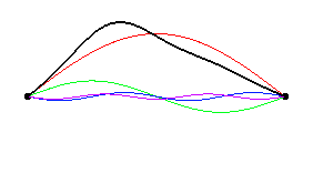
Classically its general configuration is conveniently described by a function which determines the deviations of the string from the equilibrium position at every point of the axis . For simplicity we shall assume that the ends of the string are fixed at and
| (2.1) |
In the following section we will extend our discussion to a more relevant example of a string with periodic boundary conditions - the so called closed string.
We will assume that classically the string is described by a simple linear wave equation
| (2.2) |
where has dimensionality of velocity and is actually the phase (as well as group) velocity of the waves
These are solutions of the wave equation as can be easily verified by direct substitution. Here and are arbitrary constant amplitude and phase and the dispersion relation is
| (2.3) |
It will be very useful to view the function as a collection of the coordinates describing the ”position” of the string. To emphasize this one might think of as a set indicating that is actually an index numbering different coordinates. To make it even more precise the variable can be discretized and reduced to variables as follows
Formally one should at the end let , but in practice it is enough to have much smaller than the smallest wave length of the waves which one intends to consider. The physical reasons behind the cutoff may actually be the requirement that it is much larger than the microscopic length scales related to say the distances between the constituents of which the string is built.
2.1.2 Quantum description of the string
The wave functional
Our goal is to quantize the classical string as described above. We shall use the the straightforward generalization of the canonical quantization procedure for system with few degrees of freedom like one or several particles. This means that instead of having a definite describing the string configuration we must assume that for each there is a probability amplitude which contains all the (quantum) information about the string. In particular gives the probability density to find a particular configuration .
Mathematically represents a correspondence between the set of all functions subject to the conditions Eq. (2.1) and a set of complex numbers . Such a correspondence is called a functional. Examples of functionals should be familiar to the reader already from classical mechanics where the classical action is a functional of the trajectories .
The functional is called the wave functional. Using the approximate discretized form of the functions the functional can actually be viewed as a function of variables . The variables and are fixed to to comply with Eq. (2.1).
Classically string dynamics is described by the time dependence as governed by the equation (2.2). Quantum mechanical time evolution should be described by the time dependence of the wave functional . What governs this time evolution? Continuing the analogy with the few degrees of freedom system this should be the Schrödinger equation
| (2.4) |
with the Hamiltonian operator of the string. We will now determine this operator following the standard route.
The string Hamiltonian
We will start by finding the classical Hamiltonian function of the string. For this we shall rewrite the string equation (2.2) in the Hamiltonian form. It is useful to note that this equation represents a set of coupled Newton equations for the string coordinates . This can be seen by rewriting it in a discretized form
| (2.5) |
where we used the discretized form of the second derivative
We will rewrite the second order in time wave (Newton) equation of the string as a pair of first order equations
| (2.6) |
where (as usual) the first equation is actually the definition of the momenta. As a next step let us introduce the following functional
| (2.7) |
Using it we can write the pair (2.6) as
| (2.8) |
Here the notation and stands for the variational derivative (see below) with respect to and respectively. We now show that the above equations are indeed equivalent to the pair (2.6) recalling in passing how the variational derivatives are defined and calculated.
We let the functions and in the functional (2.7) to have infinitesimal variations and . The corresponding variation due to this is
where we used integration by parts in the second term.
In analogy with the relation of the differential of a function of many variables and its partial derivatives
the functional derivatives of are by definition the functions which multiply and respectively in the expression for the variation ,
| (2.9) |
Inserting these relations into Eq. (2.8) we see that they indeed reproduce Eq. (2.6).
Basic quantum operators for the string
We shall now proceed to define the quantum mechanical operator . We will do this by first determining what are the operators corresponding to and and then replacing with them the latter in the expression (2.7) for the classical Hamiltonian.
Since in our formulation are the coordinates of the string the corresponding operator should be just the operator of multiplication by , i.e. its action on an arbitrary wave functional is
| (2.10) |
To avoid confusion we use different arguments of ’s in the operator and in . This would perhaps be easier to understand if (again momentarily) we shall switch to the notation instead of . Then the functional is just a function of the set of all variables. The action of the operator , i.e. the operator of the component the coordinates of the string is just a multiplication by with this particular . Note that in order to avoid the double subscript we here used to denote the operator.
In the same way we can determine the operator corresponding to the momentum . In the ”simplified” notations it should be which means that in terms of the functional derivatives it is
| (2.11) |
We note that the commutator of the basic operators is
| (2.12) |
This can verified by acting with the commutator on an arbitrary wave functional
Substituting the operators and in the Hamiltonian (2.7) we obtain
| (2.13) |
Armed with this explicit form of the Hamiltonian operator of our system we can proceed to solve the Schrödinger equation (2.4). Since the Hamiltonian is time independent it will be sufficient to solve the stationary equation
| (2.14) |
Knowing all its solutions will allow to find the most general solution of (2.4).
The string Hamiltonian operator (2.7) may look formidable but is actually quite simple because of its quadratic dependence on the coordinates and momenta. This of course is a direct consequence of the linearity of the string equation (2.2). As is seen from the discretized form (2.5) such equations describe coupled harmonic oscillators. The standard way of solving such problems is to make a transformation to normal modes.
2.1.3 Reminder - normal modes of vibrations
Let us recall how the transformation to normal modes is done in the general context represented by the set of N coupled equations
| (2.15) |
with masses and by symmetric matrix of elastic constants . For simplicity we shall assume in the following that all the masses are equal . The Hamiltonian of this problem is the standard sum of the kinetic and potential energies
| (2.16) |
Let us try the following solution of the equations (2.15)
where stands for real part and ’s are constants. This form assumes that all the degrees of freedom vibrate with the same frequency. Inserting this into the equations (2.15) we obtain
| (2.17) |
where we remind that we set for simplicity all . To have a non trivial solution one must demand that
| (2.18) |
which shows that is an eigenvalue of the matrix which in turns means that in general one will have such solutions which will have provided is positive definite.
Let us denote by and the set of N solutions of Eq.(2.17). The symmetry of assures orthogonality of the eigenvectors ’s with different eigenvalues . For a degenerate case i.e. if some one has a freedom to choose and to ensure that orthogonality holds also in this case. We also note that since the equations (2.17) are homogeneous at least one of the components in a given vector is arbitrary and can be used to set normalization of ’s to unity. We thus have orthonormality
The N vectors each with N components form an matrix. The orthonormality conditions (together with completeness which we do not discuss) mean that this matrix is orthogonal (unitary for complex ’s). Let us use it to make the transformation to new coordinates
| (2.19) |
Inserting this in Eqs. (2.15) (with ) and using Eqs. (2.17) one obtains
| (2.20) |
Due to orthogonality of ’s one finds that the equations for ’s are decoupled. Indeed multiplying by and summing over one obtains
| (2.21) |
The transformation (2.19) from the original coordinates to the new is called the transformation to normal modes and – the normal mode coordinates.
How does the Hamiltonian look in the new coordinates? To answer this we need to add to (2.19) also the transformation to the corresponding normal modes momenta. Since in our case it is clear that ’s transform like ’s
| (2.22) |
Inserting this and (2.19) into the Hamiltonian (2.16) we obtain using the orthonormality of ’s and equations (2.17)
| (2.23) |
where for simplicity we have set . In normal mode variables the Hamiltonian is just a collection of independent oscillators.
2.1.4 String as a collection of decoupled oscillators
Normal modes of the guitar string
We will now use the technique described in the previous subsection to transform the string Hamiltonian to a collection of independent oscillators. We are looking for the analog of the transformation (2.19) from the string coordinates to the normal modes coordinates. Since here plays the role of the index in the analog of the matrix of the transformation should be functions of defined on the interval . We denote the set of these functions by and write
| (2.24) |
where we indicated that should vanish at the end points of the string to assure the boundary conditions (2.1).
By comparing the string equation (2.2) and the coupled oscillators equation (2.15) we see that the role of the coupling matrix is played by so the functions must satisfy (cf., Eq. (2.17))
| (2.25) |
which has orthonormal eigenfunction solutions
| (2.26) |
with eigenvalues
| (2.27) |
We have fixed the coefficients in ’s so that these functions are normalized.
To conclude - the functions (2.26) represent the configurations of the string normal modes in which all the points of the string oscillate with the same frequency which depends on the wave number of the mode, Eq. (2.27). We remind that in general the relation of the frequency upon the wave vector is called the dispersion relation. It is the most important characteristic of linear waves.
Quantum mechanics of string normal modes
Using ’s we can transform the Hamiltonian operator (2.13) of the string to a sum of independent oscillators. We view the operators and as functions of and expand
| (2.28) |
Since we expand operator valued functions the coefficients and here are operators which we denoted by hats above to avoid double subscripts.
There are important relations which these operators must satisfy in order to preserve the canonical commutation relations (2.12) between and . These operators must themselves be canonical, i.e. they must obey
| (2.29) |
This can be verified in one of the two ways. We can insert the expansions (2.28) in . Using the first commutator above and the completeness relation we will obtain that (2.12) is indeed satisfied. The other two commutators simply assure that and commute at different points. The other way is to ”invert” (2.28)
| (2.30) |
and calculate the needed commutators. Incidentally the above relations also demonstrate how the operators and should act on wave functionals .
The commutation relations (2.29) mean that and are respectively coordinate and momentum operators of the normal modes of the string. As can be seen from (2.28) classically they are coordinates and momenta representing the amplitudes and their velocities of all the harmonic standing waves which the string can support.
Inserting the above expansions in (2.13) and using the orthonormality property of the set (2.26) we obtain
| (2.31) |
The Hamiltonian operator is reduced to a sum of terms each representing simple Harmonic oscillator with unit mass and frequency . It is important to observe that the underlying waves on the elastic string can only be seen in the dependence of of the oscillators on the corresponding wave vectors encoded in the dispersion relation (2.27).
Classically the simple form (2.31) of the Hamiltonian in terms of the normal modes’ dynamical variables suggests to switch the string description from to the set . Quantum mechanically we note that the relation (2.10) and the first of (2.30) implies that the operators are simple multiplication operators
Following the commutation relations (2.29) the canonically conjugate operators can be taken as
This suggests to switch to the description in which wave functionals are viewed as functions of (formally infinite number of) the variables
We now note that the terms in the sum representing , Eq. (2.31) commute between themselves on account of the last pair of commutators in Eq. (2.29). This means that the eigenfunctions of are products of the eigenfunctions of all individual terms in the sum and the corresponding eigenvalues are sums of individual eigenvalues.
| (2.32) |
The eigenfunctions are the well known harmonic oscillator eigenfunctions
| (2.33) |
where denotes N-th order Hermite polynomial. In Fig. 2.2 graphs of several of these functions are shown.

The energies (2.32) exhibit the most important result of our discussion of string quantization - that it can be viewed as a collection of independent quanta with energies . This is a consequence of two general features - string is a linear dynamical system and therefore a collection of normal modes oscillators while the quantum energy levels of oscillators are ”equidistant”, i.e. separated by equal energy intervals .
In the next Section we will consider a closed string which can support not only normal modes in a form of standing waves like the present fixed end string but also traveling waves. We will show that the corresponding energy quanta of such modes carry mechanical momentum and could therefore be considered as particles.
String ground state. The Casimir effect
The ground state energy in (2.32) is formally a sum of infinitely many ”zero point motion” terms. This is an ”ultraviolet” infinity related to the formal possibility to have waves with , i.e. vanishingly small wavelengths . In practice of course the simple description given by Eq. (2.2) ceases to be valid at atomic scales and should be replaced by a more elaborate model. As a (much more practical) alternative one could introduce a cutoff for ”allowed” normal modes in the model and limit the validity of the model (2.2) to scales .
Denoting by the largest integer corresponding to the the ground state wavefunction is a product of Gaussians
| (2.34) |
which express the ”zero point” fluctuations of the quantum string which is not at rest even in its lowest energy state.
As we will see in the forthcoming sections the ground state of the EM field is expected to exhibit similar zero point fluctuations of the fields in its ground state which is the vacuum of the theory. Is it possible to observe these vacuum fluctuations? In a 1948 famous paper Ref. [1] Casimir proposed a way to do this using what has become known as a Casimir effect. We will now explain its principle idea in the simple example of the guitar string ground state.
Let us consider what will happen with the quantum guitar string if we ”fret” it, i.e. press with an imaginary finger hard at some position so that the string will not vibrate at this point, Fig. 2.3. Obviously this changes the normal modes of the string by excluding the modes which do not vanish at . This means that the ground state energy density will change. In fact the new normal modes will consist of two families with and . The corresponding ground state energy will correspondingly consist of two parts
| (2.35) |
It is clear that for both parts are equal while for () the first term, i.e. the energy of the narrower (wider) part is smaller (larger) than the second term.
The finite cutoff frequency in the above expression ”regularizes” the (ultraviolet) divergence of the sum . To eliminate from the final result one must ”renormalize” it which can be done, cf., Ref. [2], by calculating relative to the symmetric configuration at with the result11 1 The common way of calculating is to use a ”soft” cutoff, i.e. to replace e.g. by , calculate the last sum for using with
It is seen that is symmetric with respect to and decreases monotonically as and as
| (2.36) |
The dependence on means that the function can be considered as the potential energy of the separation point of the string at and that there is a force
acting on what causes the separation between the two parts of the string (the imaginary fretting finger). This force ”tries to drive” the separation towards the end points of the string. A simple physical intuition behind this force is the imbalance of the ground state fluctuations radiation pressure on both sides of the separation point when . One must be aware however that things are more delicate as the sign of the force depends on the type of boundary conditions assumed at . For details cf., Ref. [2].
The force is called the Casimir force and its appearance is a manifestation of a Casimir effect. We will return to this effect below in the context of the vacuum fluctuations of the quantized EM field.

2.2 Quantization of Traveling Waves. Closed String
The normal modes of a string were described in the previous section are standing waves as can be most clearly seen by considering the expansions (2.28). Classically ’s and are functions each depending harmonically on time with frequency . Thus each term in (2.28) is a standing wave and .
2.2.1 Expansion in traveling waves
Periodic boundary conditions
The standing wave solution of the equations (2.25) defining the normal modes is a consequence of the fixed ends boundary conditions (2.1) for the guitar string. These were reflected in the boundary conditions in the normal modes equations Eqs. (2.25). In this section we will explore a more interesting and practical situation when the normal modes are traveling waves. This is realized if one assumes periodic boundary conditions for a string, i.e. for every
| (2.37) |
This effectively means that such string does not have ends, i.e. it is closed and equivalent to a circle. Note in passing that differentiating the periodicity condition with respect to shows that also the derivatives , , etc of are periodic. According to the string equation (2.2) this means that so are the time derivatives.
The periodic boundary conditions for are translated into conditions
replacing the fixed ends conditions in the normal modes equation (2.25). The solutions are now coming as an infinite set of degenerate pairs each with the same frequency
| (2.38) |
This degeneracy is ”compensated” by the the values of being at twice larger intervals than in the standing wave solutions (2.26) with . In real space this means that the normal modes of the closed string have integer number of the wavelengths over the string length rather than integer number of half wavelengths as it was in the fixed ends string case.
Solutions belonging to different frequencies are automatically orthogonal and we chose them to be orthogonal also within each degenerate pair. Here is a helpful integral
We also normalize them as in the fixed ends case.
As always with degeneracies the choice above is of course not unique. Another useful possibility is
| (2.39) |
again with degenerate in frequency orthogonal pairs. We will see the results of such a choice below, cf., Eq.(2.64). In the following sections we will use the freedom in specifying the degeneracy of normal modes in a closed string to find the traveling waves expansion.
Let us also note that a non vibrating constant solution exists with . This means that the string configuration in this mode is constant independent of and has linear time dependence . It describes a uniformly moving string and plays an important role in the so called super string theory. It will not be of interest to us and will not be included in our considerations.
Trying the simplest expansion
The most natural expansion using the above degenerate modes would be
| (2.40) |
with two independent sets of amplitudes and for the two degenerate modes. Inserting this in the string equation and projecting each mode leads to the decoupled equations
| (2.41) |
and the corresponding Hamiltonian
The general solution
| (2.42) |
with arbitrary initial conditions and shows however that the expansion above will be in terms of standing or traveling waves depending on these conditions.
Transforming to new normal modes variables
To obtain an expansion in traveling waves let us use the degeneracy of the two modes at every and do the following transformation
| (2.43) |
to new variables . Note that to simplify notations we dropped the subscript in the right hand side and denoted accordingly . We note that the above transformation mixes coordinates and momenta. In the Appendix we show that this transformation is canonical.
Substituting (2.43) in the expansion (2.40) we obtain
| (2.44) |
where we have combined together the sums over and modes by extending the sums to include the negative values of . We show in Appendix that this is the desired expansion in traveling waves - waves with positive and negative ’s moving in opposite directions. The hamiltonian in the new variables has the sum of independent oscillators form
| (2.45) |
with the sum extending over both positive and negarive ’s. The key point to note is that compared to (2.40) this is achieved in the expansion (2.44) by making the amplitudes of the second degenerate mode not independent but proportional to the canonical conjugate of the amplitudes of the first mode and extending the the sum to the negative k’s.
Inverting the transformation
We remark that inverting (2.44) requires some care. The simplest is to recall that and form orthonormal set for positive and use the expansion (2.40) together with the relations (2.43). This means that it is the following combinations of and which are simple projections
| (2.46) |
from which the expressions for each of the and follow by a simple calculation.
| (2.47) |
The physics of the new variables
Let us write the expressions for the terms in the expansions (2.44) as a single function. For this purpose let us transform
| (2.48) |
This gives
| (2.49) |
Since the amplitude is proportional to the square root of the energy of the mode it is a constant of the motion for the mode time oscillations. It is not difficult to show that the phase is just
Indeed writing
one finds that Eq.(2.48) is essentially a canonical transformation from to the action-angle variables for a harmonic oscillator, cf., Ref.[3], with
| (2.50) |
Mechanical momentum of the string
Apart of the Hamiltonian an important quantity describing the physics of a string is its mechanical momentum (please do not confuse this with the canonical ’s)
| (2.51) |
It is conserved by the string equations of motion (2.2) as can be seen from the following calculation. Defining the density of
we have
This is one dimensional analogue of the continuity equation which connects the time derivative of and the space derivative of the density of the Hamiltonian
Integrating this and using the boundary conditions (must use periodic not fixed ends) we obtain the conservation law
| (2.52) |
2.2.2 Quantum mechanics of the traveling waves
The basic operators. String Hamiltonian and momentum
As in the case of the fixed ends string the closed string is quantized by introducing wave functionals for the string coordinates and the operators and . The Hamiltonian operator is the same given by Eq.(2.13) since the string equations are the same. What is different are the boundary conditions which led to modified (degenerate) normal modes and the corresponding expansions (2.44).
Using these expansion for the operators
| (2.53) |
we are led to the canonical commutators for the traveling waves amplitudes
| (2.54) |
These of course follow from the basic commutators (2.12) and the expressions (2.47). The Hamiltonian operator in terms of ’s and ’s has the same form of decoupled oscillators
| (2.55) |
Quantum mechanically the string momentum , Eq. (2.51), becomes an operator
| (2.56) |
As usual with products of non commuting operators, here and , one must use a symmetrized expression.
The operator is the generator of translations
Indeed using the basic commutators (2.12) one can easily verify that
| (2.57) |
as it should be for the generator of translations.
Inserting the expansions (2.2.2) in the momentum we obtain
The eigenstates. Energies and momenta of traveling waves quanta
The traveling waves Hamiltonian (2.55) has the same decouple normal modes oscillators form as the one for the standing waves (2.31) so formally its solutions have the same form as (2.32)
| (2.58) |
with familiar harmonic oscillator eigenfunctions , Eq. (2.33). There are however important differences.
Since the traveling waves energy quanta are doubly degenerate with respect to the sign (direction) of k. Even more profound is that these quanta also carry momentum. Indeed comparing the expression (2.2.2) for the string momentum with the Hamiltonian one observes that has the same eigenfunctions (not surprising) with the eigenvalues22 2 The presence of terms in this expression helps to cancel the ”zero point motion” term present in the expression for the energy.
| (2.59) |
Each quantum has ”mechanical” momentum . So the closed string can be considered as a collection of traveling waves ”quasi”particles with energy momentum relation
| (2.60) |
It is useful to pay attention that this result can be viewed (obtained by a shortcut) as a consequence of the three fundamental relations - two basic quantum mechanical relations - the Plank-Einstein and the de Broglie and the string dispersion relation . In a similar way we will find below that the quanta of the EM field will be particles (photons) with energy-momentum relation i.e. of massless relativistic particles. The quanta of the Schrödinger field will have , i.e. the energy-momentum relation of non relativistic particles.
Transformation to creation and annihilation operators
In practice it is very convenient to introduce creation and annihilation operators in the standard way
| (2.61) |
Using these operators we can write the Hamiltonian
| (2.62) |
and its eigenstates
| (2.63) |
Great advantage of using and operators rather than and is the simplicity of the ”action” of these operators on the ”number states”, i.e the states with a fixed numbers of quasi particles in each normal mode. Schematically
In detailed notation
One says that the operators and create and destroy quasi particles of energy and momentum .
It is useful to express the field operators in terms of and . Using (2.2.2) we obtain
| (2.64) |
which are sums of terms which either create a quantum with momentum or annihilate one with the opposite momentum .
2.3 Quantization of the EM Field
The quantization of the electromagnetic field follows the same route as with the simple string above. The classical equations of the field are the Maxwell equations. We will now cast them into Hamilton form and identify the Hamiltonian and the canonical coordinates and momenta of the field. We will then replace them by operators with canonical commutation relations acting on the appropriate wave functionals.
2.3.1 Hamilton form of the Maxwell equations
The Maxwell equations have the familiar form33 3 In this Chapter we use the SI system of units.
| , | (2.65) | ||||
| , |
Here is the light velocity and is a constant called vacuum permittivity which is related to our choice of the SI measurement unit system.
The Maxwell equations describe the EM field configuration for a given distribution of the electric current and density of electric charges. Assuming that we are dealing with a system of charges and denoting by , their positions and velocities we have
| (2.66) |
These expressions must be supplemented by the mechanical equations of motion for the charges as they move in the given and . These equations are just the Newton equations for the charges
| (2.67) |
The coupled equations (2.65), (2.66) and (2.67) provide the complete system which determines how the positions of the charges and their motion determine the EM field and how this field determines the motion of the charges. Our first goal will be to cast this system in the Hamiltonian form thereby determining its canonical variables and the Hamiltonian.
Vector potential. The gauge
We start by noting that the first pair of Maxwell equations (2.65) does not involve time derivatives. They are in a sense constraints on the possible functional dependence of and . Both constraints are easy to resolve. The condition means that there are no magnetic charges in nature and that B can be represented as a curl of an arbitrary vector function
| (2.68) |
which is conventionally called the vector potential. In the chapter where we considered the motion in an external EM field we have seen that the quantum mechanical formulation was impossible without an explicit use of this function. Also presently we will find that the quantization of EM field can not avoid using A.
The second pair of the Maxwell equations consists of dynamical equations. Inserting Eq. (2.68) in the first of these equations we obtain
| (2.69) |
Here is (in non relativistic parlance) the ”scalar potential” which together with A completely determine the fields E and B. The potentials A and are not uniquely defined. We can choose instead different function and related to and A by the gauge transformation
| (2.70) |
with arbitrary function . We shall use this freedom and take to be identically equal to zero and write
| (2.71) |
This choice is called ”working in the gauge”. Importantly this choice does not exhaust the full gauge freedom. We can still add to A a gradient of a time independent function without changing our assumption.
Inserting (2.68) in the last of the Maxwell equations (2.65) we obtain
| (2.72) |
Using (2.71) this equation becomes
| (2.73) |
Regarding the 2nd time derivative on the left as acceleration of one can view the above equations as coupled Newton equations for the degrees of freedom . In this view at every point in space there are three such degrees of freedom (field coordinates) which can symbolically be represented as . The 3 dimensional vector index is and r is running over all points in the 3 dimensional space in a way similar to running over points of the axis in the example of a string. The coupling between different is via complicated combination of second order vector derivative connecting different vector components of in neighboring points.
The last term in (2.72) is the ”force” acting on the field coordinates on the part of the matter. Ignoring this force for a moment (i.e. considering the EM field in an empty space region) we can view the coordinates as representing coupled oscillators. This is because the above equation without the last term is linear. Although complicated from the vector analysis point of view the derivatives combination is a linear operation.
The Hamiltonian
Continuing with the ”mechanical” interpretation of the EM field dynamics we notice that the pair of the 1st order equations (2.71) and (2.72) without the last term can be regarded together as Hamilton equations with the following field Hamiltonian
| (2.74) |
and canonical variables as coordinates and as momenta. We will verify this in a moment but first we note that perhaps the simplest way to guess the expression of the Hamiltonian is to notice that on account of Eq. (2.71) the first term in it has the form of the kinetic energy. One can determine how it changes with time by forming a scalar product of the left hand side of (2.72) with E. Multiplying the first term on the right hand side (remember we still are ignoring the current term) with the equal quantity we can integrate both sides over r. After simple manipulations44 4 Here are the details one can show that the change in time of the kinetic energy is equal to minus the change in time of the second term in which has the meaning of the potential energy. This of course verifies that is conserved, .
Returning to the Hamiltonian (2.74) we form its first variation
where we performed integration by parts in the second term. From this it follows that
| (2.75) |
showing that the Hamilton equations with this Hamiltonian and canonical variables and
| (2.76) |
indeed coincide with Eqs. (2.71) and (2.72) without the current term.
Let us now show how to account for the current term and the dynamical Newton equations (2.67) for the charges. Here we are guided by our knowledge of the Hamiltonian of charges moving a given EM field (cf. Chapter Motion in External EM Field). We simply add it to above and obtain
| (2.77) |
Using exactly the same calculation as in the chapter Motion in External EM Field we can show that the Hamilton equations
| (2.78) |
are equivalent to the Newton equations (2.67). Let us now consider the first variation of the last term in (2.77) with respect to . We obtain
where is the current as defined in Eq. (2.67) with
With this result the second equation of (2.76) with replaced by the full (2.77) now reads
| (2.79) |
reproducing the full equation (2.72). We also note that since the second term in the full does not depend on E the first equation in (2.76) remains unchanged when is replaced in it by .
2.3.2 Canonical quantization
Having established the canonical structure of the theory we can now quantize it. Attentive reader should have noticed that we have not yet accounted for the first equation in the set (2.65) expressing the Gauss law. We also seem to be missing from the Hamiltonian (2.77) the regular Coulomb interaction energy between the charges . We will address these issues shortly but meanwhile let us proceed with the quantization.
Moving from classical to quantum description we recognise that the coordinate set of our system consists of the vector potential (i.e. 3 vector components in each point of the position space, i.e. variables ) and 3N vectors of the particles’ positions. Accordingly we introduce the wave functional of the field which also depends (is a function of) the N particles’ positions and the
| (2.80) |
This should be viewed as a correspondence between all field configurations and set of N particles’ positions and (in general) complex probability amplitudes which in general change with time.
The physical operators are constructed from the corresponding classical quantities by the canonical substitution
| (2.81) | |||||
where we accounted for the fact that it is the combination which is canonical to not just . Using the equality
it follows that the field operators obey the commutation relations
| (2.82) |
The time dependence of the wave functional/function is governed by the Schrödinger equation
| (2.83) |
in which the Hamiltonian operator is obtained by replacing in the classical expression (2.77) the fields , and the particle variables , by the corresponding operators (2.81),
| (2.84) |
The above Hamiltonian does not depend on time as we are dealing with a closed EM field + matter system. The energy is therefore conserved and quantum mechanically we can reduce in the standard way the solution of the above time dependent Schrödinger equation to solving the static equation
| (2.85) |
This is a complicated equation for the coupled field-matter system. No exact solution is possible. We will discuss approximate solutions below. But before that we have to clarify several formal but very important issues which will allow us to somewhat simplify the problem.
2.3.3 Gauge invariance
The Gauss law
We will now show that the Hamiltonian formulation presented above neatly accounts for both the Gauss law and the Coulomb interaction between the charges. The key to this is to observe that the Hamiltonian is invariant under the gauge transformation
| , | (2.86) | ||||
| , |
with an arbitrary time independent function . This is the residual gauge transformation we have briefly mentioned after Eq.(2.72).
The symmetry of under (2.86) is the result of the way the vector potential enters it, i.e. only via the combinations and . It is a local symmetry meaning that it is characterised by parameters which depend on r. Schematically there are parameters corresponding to the ”number” of points in the 3D space of vectors r. As we will show below the generators of this symmetry are
| (2.87) |
Their dependence on r means that there are generators corresponding to parameters in (2.86).
Classically expressions corresponding to the generators of symmetries of the Hamiltonian are conserved by the Hamilton equations. Momentum and angular momentum are of course the classic examples of such conservations. Accordingly let us show that equations (2.71), (2.72) and (2.67) conserve the above expression for the generator when it is taken as classical and when E and in it are allowed to evolve according to these equations. We have
| (2.88) |
where we used Eq.(2.72) and the continuity equation for the charges.55 5 Continuity equation is a general relation between and given by (2.66)
The vanishing of means that local quantities form a constant, time independent function of r. It is natural to denote this function by
and interpret it as a density of fixed static electric charges. We notice that these charges appear in addition to the dynamical charges described by the equations (2.67). Under normal circumstances there are no such extra static charges. In fact there presence would violate such symmetries as translational, rotational, Lorenz. So one should assume that . Using this in the above relation we recover the Gauss law.
Quantum mechanics of the gauge transformation
Let us work out the quantum mechanics of the gauge transformation (2.86) . What we want to show is that it is generated by the operators , Eq. (2.87), i.e. that the following relations hold
| (2.89) |
As usual it is enough to consider the infinitesimal for which the left hand side reduces to
| (2.90) |
Here we omitted the identity term and used
| (2.91) |
and
| (2.92) |
Now we do the integration by parts and use the delta function
| (2.93) |
obtaining exactly what is needed to get the dependent term in the right hand side of Eq.(2.89).
Thus operators are indeed the generators of the gauge transformation. Since the Hamiltonian operator is invariant under this transformation one must have that commutes with
| (2.94) |
As in simpler quantum mechanical systems this means that and have common eigenfunctions. We write symbolically
| (2.95) |
where we denoted by the eigenvalues of the operators . As in the classical case the meaning of is the density of static (”background”) electric charges. They are ”background” because they are not a part of the dynamics. Just sit there as a part of initial conditions. Their presence would violate basic symmetries (translational, rotational, Lorenz) so the physics dictates that one must select only the eigenfunctions which belong in the ”sector” of the system Hilbert space for which
| (2.96) |
In other words - the gauge invariant sector.
Separating the longitudinal components of the fields
In the Hamiltonian formulation the electromagnetic field has degrees of freedom which in our formulation are described by the coordinates and the corresponding momenta , . Using the local gauge symmetry (2.86) one can eliminate one third of these degrees of freedom. For this reason let us represent the functions and as sum of the so called transverse and longitudinal components
| (2.97) |
where , , and satisfy
| (2.98) |
Such a representation is possible for any vector field. This can be shown (and the origin of the names longitudinal and transverse understood) using Fourier expansions. Let us take for example and expand
| (2.99) |
For convenience in order to have discrete values of k we consider the fields in a large but finite volume. The precise boundary conditions are not important for this discussion.
The Fourier amplitudes are vectors. Their directions in principle bear no relation to the direction of the corresponding wave vectors k. We can however represent each of them as a sum of two vectors which are parallel and perpendicular to ”their” k
Using this we can write the Fourier expansion as a sum
| (2.100) |
Using
we see that the two terms in the Fourier expansion of are respectively and as appear in (2.97).
We note also that longitudinal components of the vector fields can be written as a gradient of a scalar function. Therefore we can write
| (2.101) |
where two scalar functions and - fully determine the longitudinal components and respectively. As will become clear in the next section is the scalar electric potential so familiar from the Coulomb and other electrostatic problems.
Recovering the Coulomb interaction. Resulting Hamiltonian
Inserting the above expressions for and in the Hamiltonian (2.77) we obtain
| (2.102) |
We have transformed to . The mixed term containing does not appear since it vanishes as can be seen after integrating it by parts
As a last step in transforming we note that the Gauss law allows to express in terms of
| (2.103) |
We see that in this formulation the familiar scalar potential appears in the longitudinal component of the electric field and is completely determined by the density of the charge. This allows to express the term in containing as
This is just the Coulomb interaction between the charges in and can be written using the expression for given in (2.67) as
| (2.104) |
where are constants which express the Coulomb self-energy of each particle. They diverge for point particles. We will not deal with this in details but assuming that particles have small but finite sizes (cutoffs) we will simply disregard this constant term.
To conclude, the Hamiltonian has the form
| (2.105) |
where we defined the radiation and the Coulomb interaction parts of the Hamiltonian
| (2.106) | |||||
It is often convenient to write this Hamiltonian as a sum of three parts
| (2.107) |
where is given by (3.25) and
| (2.108) | |||||
| (2.109) | |||||
Note that when switching to operators there will be no operator ordering ambiguity in the term since the difference, i.e. the commutator
An aside - separating transverse and longitudinal Maxwell equations
Let us now examine how the Hamilton (Maxwell) equations (2.71) and (2.72) look in terms of the transverse fields , . One can see that each equation separates into two relating separately the transverse and longitudinal components
| (2.110) | |||||
The last equation is equivalent to the continuity equation for the current
| (2.111) |
as can be see by taking divergence of both parts and using the Gauss law for . The equation , shows how the longitudinal component of A which does not enter the Hamiltonian (i.e. is the ”cyclic” coordinate) develops in time for a given which in turn is determined by the Gauss law via the charge density. One can see this as analogous to say the motion of the angular coordinates in a spherically symmetric problem as determined by the (conserved) angular momentum.
2.4 Photons
2.4.1 Field oscillators
In the present and following sections we will disregard the radiation-matter interaction and will concentrate of the radiation part described by . Since this Hamiltonian is quadratic we will continue as in the case of a string. We will impose periodic boundary conditions and will expand and in terms of traveling waves. As we will see will become a sum of decoupled oscillators so the traveling waves are the normal modes of the radiation.
Expansion in traveling waves
Following the string example, cf., Eq.(2.44) and the footnote66 6 For easy comparison we reproduce this expansion here below we expand the field canonical coordinates and momenta and , cf. Eq. (2.76) in a large volume
| (2.112) | |||||
with vector expansion coefficients and . To make the above expansions more symmetric with respects to the appearance of we changed our canonical variables to
The periodic boundary conditions lead to discrete values of the wave vectors
| (2.113) |
where we assumed the volume to be a cube, i.e. have the same length, width and height each equal to .
The more conventional form of the expansion Eq. (2.112( found in the literature (cf., cf. Landau and Lifshitz, Classical Field Theory, Sec.52 or Ref. [7] ) is written in terms of canonically transformed variables
| (2.114) |
which for the transverse components of the fields results in
| (2.115) | |||||
The transversality of and means that the vectors and are always orthogonal to the corresponding k,
It is convenient to use a pair of fixed unit polarization vectors , with
| (2.116) |
so we can write
| (2.117) |
We now insert expansions (2.115) and (2.117) into the Maxwell equations for the transverse component, i.e. into the 1st and 3rd equation of the set (2.110) in the absence of the current (recall we are discussing pure radiation). We obtain in the straightforward manner separate linear equations for and
| (2.118) |
One clearly sees that these are Hamilton equations of harmonic oscillators labeled by each with the Hamiltonian
| (2.119) |
and and being the generalized coordinates and momenta. One could also obtain this by inserting expansions (2.115) and (2.117) into to find
| (2.120) |
It is seen that indeed we represent as a sum of decoupled oscillators with frequencies given by the well know dispersion relation of the EM waves. There are two oscillators with different polarizations for each k. Since depends on the magnitude of all the oscillators with have the same frequency.
Field wave functions and eigenstates. Photons appear
We now turn to the quantum mechanics of the radiation. It is the easiest to do this in the decoupled eigenmodes of the field as encoded in the Hamiltonian (2.120). Instead of classical time dependent variables and we consider wave function which contains all the quantum information. This is ”extracted” by using operators for every physical quantity which are build of two sets of basic operators of the ”coordinate” and ”momentum”.
| (2.121) | |||
All in the usual way as in quantum mechanics of mechanical systems.
The time dependence of is governed by the Schrödinger equation
| (2.122) |
with the Hamiltonian operator obtained from Eq. (2.120) by replacing in it the coordinates and momenta with the corresponding operators
| (2.123) |
The most important solutions of the Schrödinger equation are the stationary states which are the eigenstates of
| (2.124) |
Since is a sum of independent terms each representing an oscillator the eigenvalues of are sums of eigenenergies of independent oscillators
| (2.125) |
The corresponding eigenfunctions are products
| (2.126) |
where are the standard eigenfunctions of a harmonic oscillator, cf., Eq.(2.33), with unit mass and frequency .
As in our discussion of the string quantization (and actually in the quantization of any linear dynamical system) we find that the EM field can be viewed as a collection of energy quanta
in its normal modes. In the following sections we will show that these quanta have all the characteristics of particles. They carry momentum, angular momentum and spin and have energy-momentum relation of massless particles moving with the speed of light, cf., Eq.(2.141). These quantum particles are photons.
Focusing on the details we note that the EM modes are 3D vector waves. In our developments we have chosen them as plane waves with wave vectors k and polarisations . But let us note that the eigenfrequencies of these modes and as a result the energies of the quanta depend only on the magnitude of k, i.e. on the wavelength and not on the direction of the vector k and the polarisation of the modes.
As with the ordinary matter particles with e.g. this means that there is a continuum degeneracy of the modes and therefore of the quantum mechanical states of the (free) photons. This degeneracy results in a freedom to change the basis states with a given energy from the vector plane wave (like we did above) to e.g. spherical (vector spherical!) or cylindrical (vector cylindrical!) etc waves. The quantum numbers will then be replaced by appropriately changed ones like replacing in the scalar waves. A recent reference to the vector spherical waves is e.g. Ref.[4].
The wave function of the vacuum. The Casimir effect
The ground state of the EM field is the vacuum of the theory in the absence of matter and other quantum fields. Its wave function is the product of Gaussians familiar from our discussion of the guitar string, Eq. (2.34),
| (2.127) |
It provides perhaps the simplest example of quantum vacuum fluctuations of field degrees of freedom in a quantum field theory.
Can one observe these fluctuations? In a ground breaking paper, Ref.[1], Casimir addressed this issue. He suggested that such fluctuations induce ”attraction between two perfectly conducting plates”. On such plates the parallel to the plates components of the electric field must vanish so that the field normal modes for which this doesn’t happen will be excluded from the field degrees of freedom and consequently from the vacuum fluctuations. This is schematically illustrated in Fig.2.4. The density of the normal modes frequencies between the plates will be smaller than in the free space outside.
We have considered a one dimensional version of this effect in the context of the quantum guitar string, Sec.2.1.4. We have shown there that it leads to an attractive force between the (analogue of) the plates with the more narrow spacing than that of the other part of the string. The same happens in the realistic 3D case with quantized EM field. Casimir calculations predicted that an attractive force per unit area (pressure) at plate separation is given by
Note that the inverse quartic dependence on the distance is most unusual in physics. It is also worth mentioning that for certain special combinations of the plates materials, the Casimir force can be repulsive. The results obtained by Casimir were later extended to various geometries of the plates and his predictions were confirmed experimentally, cf., Ref.[6].

Photon creation and annihilation operators. Field operators
In practice it is convenient to introduce creation and annihilation operators of photons in the standard way
| (2.128) |
Using these operators we can write the Hamiltonian
| (2.129) |
and its eigenstates
| (2.130) |
Great advantage of using and operators rather than and in dealing with photons is the simplicity of the ”action” of these operators on the ”number states”, i.e the states with a fixed photon numbers in each normal mode. Schematically
In ”full glory”
One says that the operators and create and destroy(annihilate) photons.
It is useful to express the operators of the fields (2.115) as well as in terms of the creation and annihilation operators
| (2.131) |
Once the longitudinal components of the fields and were separated the remaining transverse parts and do not obey the canonical commutations (2.82). Rather the delta function there gets replaced by the so called ”transverse” delta function cf., Ref.[7], Ch.İII.A.1.
2.4.2 Photon momentum
In this subsection we will consider the operator of the momentum of the EM field . Using it we will be able to show that photons are not just ”portions” of energy of the EM field but that they also carry a ”corresponding” portion of its momentum. Moreover the relation between the energies and momenta of these portions are as of massless particles traveling with the speed of light.
Generators of translations in the matter-field system
Quantum mechanically it is probably the easiest to guess the expression of the momentum by recalling that it is the generator of infinitesimal translations. For the interacting system of particles (matter) and EM field described by the Hamiltonian (2.84) the operation of infinitesimal translation is the transformation
| (2.132) | |||||
Therefore the(vector) momentum operator of the system should be such that for each of its component , the commutators hold
| (2.133) |
| (2.134) |
It is actually very easy to guess what such should be
| (2.135) |
where and the ”h.c.” abbreviation stands for ”hermitian conjugate”.
Indeed the first term has the required commutator with while commuting with and and the second term commutes with and satisfies
where in the last line we used the integration by parts.
Let us recall the classical expression for the conserved momentum in the presence of the EM field. On the basis of the Maxwell and Newton equations Eqs.(2.65 - 2.67) one finds that
| (2.136) |
is the conserved total momentum of the field-matter system
| (2.137) |
cf. p. 61, in Ref.[7] or a less formal text - Ref.[8]. In Appendix 2.5.3 below we show the equivalence of the expressions (2.135) and (2.136).
Momentum of the EM radiation
In the absence of charged particles we can use and replace by the transversal in the field part of the momentum in (2.135). The same can be done with in it. Indeed the longitudinal part of can be written as a gradient . Thus it contributes (after the replacement ) the term
in . This term is however zero as can be seen by integrating by parts in the right hand side and using .
Thus we can write the momentum of the ”pure” radiation as
| (2.138) |
Inserting expressions for the operators and one obtains
| (2.139) |
where we used 77 7 There is a subtle point here - this sum diverges and must be regularized by, say, assuming a cutoff at some large . . As it should commutes with the Hamiltonian . Its eigenvalues are
| (2.140) |
We can see that every state with quanta has momentum so that every energy quantum with carries momentum . Using the dispersion relation of the (classal) light waves (EM normal modes) we find the energy-momentum relation of light quanta
| (2.141) |
i.e. of the massless particle moving with the light velocity.
2.4.3 Common states of light
Number states
These are just the eigenstates of the , cf., Eq. (2.129). Although most natural from the formal point of view they are highly nonclassical and in fact are extremely hard to produce ”on demand”88 8 E.g. M. Oxborrow and A.G. Sinclair, Contemp. Phys. 46, 173 (2005).. Number states are states of well defined energy but not of the states of well defined EM field. As an example consider a single mode of the electric fields, i.e. just one term with a given in the expression for in (2.131) and calculate
| (2.142) |
and
| (2.143) |
so that the everage value of is zero while the fluctuations grow with the number of photons.
Quantum mechanics behind the classical EM field. Coherent states of light
The correct description of the world is quantum mechanical while the classical physics is just an approximation. So it is natural to ask what is the quantum mechanical state behind the classical EM field? Since the quantum mechanical operators of electric and magnetic components and of the field are non commuting there is no state in which they both have definite values.
Under these restrictions the appropriate quantum state behind the classical EM field must be such that the averages, i.e. the expectation values of the field operators
will be developing in time as solutions of the classical Maxwell equation and be ”classically large” i.e. much larger than the quantum uncertainties i.e. the standard deviations of these fields from the averages..
It is not hard to find the state with the above properties for a free EM field. Since such a field can be represented as a collection of independents modes it is useful to start by considering a simple case of just a single mode with a given wave number k and polarisation . Concentrating on the electric field we have the operator
| (2.144) |
The quantum mechanics of and its non non commutativity with is ”encoded” in the canonical non commuting pair of the operators . Their dynamics (for a free field) is simple - just that of harmonic oscillator, cf., Eq. (2.123).
So the task is to find a quantum state of harmonic oscillator, i.e. solutions of the Schrödinger equation
| (2.145) |
for which the averages
obey the classical equations of the harmonic oscillator
| (2.146) |
and have smallest possible quantum uncertainties.
Such a state was first discussed by Schrödinger already in 1926 and has a name - coherent state. Its common formal definition is that it is an eigenstate of the annihilation operator
| (2.147) |
with eigenstates labeled by the eigenvalues and where we used the coordinate representation of
Note that since is non hermitian ’s are in general complex valued99 9 There are many unfamiliar features of states as a result of this. Like non orthogonality at different ’s or over completeness. This will be partly covered in the Appendix. Also note that for the coherent state is just a ground state of the harmonic oscillator
| (2.148) |
The properties of the coherent state are discussed in the Appendix of this chapter. It is shown there that coherent state is a wave packet the dynamics of which is such that the averages
| (2.149) |
move along the corresponding classical trajectories with uncertainties obeying the minimum uncertainties relation
| (2.150) |
It is useful to schematically present this picture in the classical phase space as is explained in Fig. 2.5.

Let us briefly consider how the EM field ”looks like” in a coherent state. Consider a single mode (2.144) written in terms of the photon and assume it is in a coherent state . Then
| (2.151) |
where we used the results (2.168, 2.169) from the Appendix. This expression for the average has the form of a classical field. Its amplitude is controlled by , cf., the radius of the classical trajectory in Fig. 2.5.
Calculating
| (2.152) |
we obtain for the quantum fluctuations
| (2.153) |
which is independent of the magnitude of the average, cf., again Fig. 2.5. So for the electric field than the quantum scale of the fluctuations the field can be viewed as classical.
Thermal light
Thermal radiation is radiation in thermal equilibrium, which means (as is usual in quantum statistical physics) that this radiation is described not by a wave function (or rather wave functional) but by the density matrix. This density matrix is diagonal in the eigenenergy basis
| (2.154) |
with the probabilities given by the Boltzmann factor
which of course is equivalent to saying that the radiation power follows the Plank law. Just to remind - by using
separating exponentials in and into products with different and summing over for each in one obtains
| (2.155) |
and . The average energy per mode is
and the Plank spectral energy density
with .
Such a spectrum is an idealization of a radiation spectrum emitted by matter sources which by themselves are in a thermal equilibrium and moreover the radiation which they emit ”has enough time” inside the matter to reach equilibrium with it. The major factors ”distorting” such spectra are layers of matter (like sun and earth atmospheres) between the equilibrated matter-radiation system and the observer. If such layers have different temperature and are too thin the light will ”have no time” to re-equilibrate as it passes through them. The layers will just absorb some of the passing radiation at particular wave lengths depending on their chemical composition. This will produce the corresponding ”absorption lines” in the radiation spectrum. Hot excited atoms, molecules, etc, inside the layers will also emit and add non equilibrated light at particular wavelengths producing the ”emission lines”. Example of the observed solar radiation spectrum, cf., Fig. 2.6 provides a good illustration of these features.


2.4.4 Photon angular momentum and spin
Using the Maxwell and Newton equations (2.65), (2.67) together with the charge current and density (2.66) one can show (cf., Ch 1A in Ref.[7]) that the conserved angular momentum of the matter-field system is
| (2.156) |
Comparing with the expression (2.136) for the matter-field momentum both terms have intuitively clear meaning.
It is important to note that as is usual with the definition of angular momentum the expression (2.156) refers to a specific point - the origin of the chosen coordinate system - with respect to which J is calculated. This of course can be easily changed by replacing and with an arbitrary vector in both terms of J respectively. This change leads to a straightforward generalisation of the classical mechanics relation for such transformations of angular momenta
Generators of rotations in the matter-field system
Consider infinitesimal rotations of the coordinate system
where as usual the magnitude of the vector is equal the rotation angle and it is directed along the axis of rotation (right hand rule). We want to determine how the wave functional changes under this transformation.
Let us start by recalling that a scalar field change obeys the intuitive rule
saying that the values of the rotated field at rotated points are the same as non rotated field in original points r. Using and dropping the prime in on both sides can write
| (2.157) | |||||
For a vector field one also has to rotate the field itself
which gives (after dropping the prime on )
| (2.158) | |||||
As in the scalar field case the last term corresponds to the ”orbital” rotation with while in the Appendix below we show that the additional second term is (not surprisingly) a rotation of the components of the vector A with spin one matrices.
Let us now examine what happens to a wave functional when its argument is transformed as in (2.158). To simplify things we leave out the particle coordinates aince the part of the rotation generator for them is obvious. Have
where we used the expression for as defined in (2.81). Using the explicit form of from (2.158) we can write for the integral in the second term
From this we can read off the generator of rotations for the field part. It can be written as a sum of two parts - spin and orbital
| (2.159) |
with
| (2.160) |
where we indicated that A in this expression should be regarded as operator (although it is diagonal, , in the representation of .
Note that in the expressions for and we were free to commute components to the left. Indeed in the commutator of and is proportional to the derivative of the delta function
which vanishes at . In only different i.e. commuting components and with enter in their vector product.
2.4.5 Photon parity and photon statistics
The vector potential is a polar vector - it changes it sign under parity transformation
| (2.161) |
This property of is the basis of the statement that the photon, i.e. the quanta of the vibrations of have negative parity. We note that at this stage this is a fairly cryptic statement which becomes clear when photon emission by matter system is studied (cf., later in the course).
Photons are bosons! This too is a somewhat cryptic statement at this stage. It will become clear when dealing with the second quantitation formalism of the Schrödinger field in relation to quantum many body systems. Here we only remark that one can have any number of photons in the same state, i.e. in the same mode characterised by quantum numbers.
One can calculate the commutator of the operators of the electric and magnetic fields and and find that they do not commute. This have all the usual quantum mechanical consequences. In fact in tutorials and home works we/you will deal with issues related to questions like ”what is the electric/magnetic field of a photon?”
2.5 Appendix
2.5.1 Details of the standing to traveling waves transformation
What does the transformation Eq. (2.43) achieve
Let us start by noting that the Hamiltonian for a given has the same form in the new variables
and due to their canonicity (cf., below) the dynamical equations for are the same as for so their solutions have the same form as in Eq. (2.42). Now both terms in this solution give traveling waves when inserted in the expansion (2.44). Indeed have for the first terms in these solutions when inserted in the expansion for
and for the second terms
These traveling waves are ”running” in the positive or negative -direction depending on the sign of .
Verifying canonicity
Our transformation from the standing waves expansion (2.40) to the traveling waves (2.44) amounted to transforming from phase space variables to , Eq. (2.43). Let us now check the canonicity of this transformation.
Let us recall that in a mechanical system described by a set of generalised coordinates and momenta the transformation to a canonically conjugate set must satisfy
where denote a complete differential. In our case the set is and we are transforming to . We obtain
It is instructive also to verify the canonicity of the general transformation (2.44). In this case the set is , the sum over is integral over and we are transforming to . So we have
which shows the canonicity of and .
2.5.2 Details of the coherent states
Useful averages. Minimum uncertainty
It easy to find an explicit solution of the equation (2.147). But before doing that it is useful first to calculate the following averages
| (2.162) |
which give
| (2.163) |
Also have
| (2.164) |
and
| (2.165) |
which shows that the coordinate and momentum uncertainties in this state are independent of
| (2.166) |
which in turns means that for large (classical) values of and , i.e. for large , cf., Eq. (2.163), the quantum uncertainties are negligible. The actual values of and show that is a minimum uncertainty state, Eq. (2.150).
Dynamics of coherent states
Let is now consider the dynamics of a coherent state, i.e. find
For this we use the Heisenberg representation of and the corresponding Heisenberg equation which is easily solved
| (2.167) |
This gives
| (2.168) |
which shows that remains a coherent state with
| (2.169) |
In terms of the corresponding and
which coincide with the solution of the classical equations (2.146).
Explicit expressions. Ground state of a shifted harmonic oscillator
Using the explicit expression (2.148) for the coherent state at it is easy to find solutions of Eq. (2.147) for a general by using the decomposition (2.163) in (2.147)
and noticing that this equation is similar to the one with , Eq. (2.148), but with a shift and a dependent phase
| (2.170) |
It clearly can be regarded as a ground state of a shifted harmonic oscillator, i.e. of
| (2.171) |
This observation is important for a qualitative discussion of the laser light.
Let us note that the coherent state can also be written as an expansion in a complete set of number states, i.e. the harmonic oscillator eigenstates
Acting with we obtain
Find from normalization
so
| (2.172) |
It is also easy to calculate the overlap
showing non orthogonality of different states. The set is over-complete but satisfies a useful resolution of unity relation
which is easy to prove by using the expansion (2.172) and changing to polar coordinates in the integral.
2.5.3 More on the EM field momentum
Relation to the classical expressions for the matter-field momentum
Classical expression (2.136) can be written
| (2.173) |
It is related to the integral of the Poynting vector, cf., the reference to the Feynman lectures given above for the physics discussion of this result.
Let us write this expression in components (using the Levi-Civita tensor and the summation convention)
| (2.174) | |||||
so that
| (2.175) |
where we integrated by parts in the last equality. Using the Gauss law this gives
| (2.176) |
where we used to integrate.
Field momentum in terms of the transverse components
Both terms in the expression (2.136) are separately gauge invariant. However the two terms in the transformed expression (2.177) are not. Only their sum is. We can repair this if we repeat the calculation (2.175) but first replacing A by in the starting left hand side. This will lead to the same expression as (2.177) but with replacing A in it
Now both terms are gauge invariant. We can moreover in the second term replace by . Indeed writing
and using
we express
| (2.179) |
In the absence of the charged matter (i.e. when all ’s are zero) the field part of this momentum becomes the momentum of the free radiation as we have already derived in (2.138).
2.5.4 More on the EM field angular momentum
Relation to the classical expression
See Ref.[7], Complement .
Spin 1 part of rotations of a vector field
We can write the 2nd term in Eq. (2.158) as
where the matrices
are spin 1 matrices written in cartesian components basis rather than in the more familiar spherical components basis ( )
i.e. .
One can easily verify that the commutators indeed have the correct form
| (2.180) |
For this must prove that
is equal to
Have
which indeed is equal to
References and Guide to Reading.
- [1] H. B. G. Casimir, Proc. K. Ned. Akad. Wet. 51, 793 (1948)
- [2] T. H. Boyer, American Journal of Physics 71, 990 (2003)
- [3]
Action-angle Variables. University of Rochester.
https://phys.libretexts.org/@go/page/9653 - [4]
G. Kristensson. Spherical Vector Waves. Lund, 2014
https://www.eit.lth.se/fileadmin/eit/courses/eit080f/Literature/book.pdf - [5]
K. Kingsbury, The Casimir Effect, Version 3, A Comprehensive Exercise, 2009.
https://aphyr.com/media/comps.pdf - [6] A. Stange, D. K. Campbell, and D.J. Bishop, Science and technology of the Casimir effect. Physics Today 74, 1, 42 (2021);
- [7] C. Cohen-Tannoudji, J. Dupont-Roc, G. Grynberg, Photons and Atoms: Introduction to Quantum Electrodynamics, 2004 Wiley.
- [8]
http://www.feynmanlectures.caltech.edu/II_27.html.
Chapter 3 Photon-Matter Interactions
This chapter is the continuation of the chapter ”Quantum Mechanics of Electromagnetic Field”. We will use the quantum description of the EM field discussed there to provide several simple examples of how photons are emitted and absorbed by quantum matter systems.
3.1 Interaction Hamiltonian
3.1.1 Separating the interaction terms
As was shown in the chapter ”Quantum Mechanics of Electromagnetic Field” the Hamiltonian operator of the EM field interacting with (non relativistic) matter is
| (3.1) |
with
| (3.2) | |||||
| (3.3) |
and
This expression can be written as
| (3.4) |
with
| (3.5) | |||
and
| (3.6) | |||||
| (3.7) |
The expressions for and depend on the coordinates and momenta of the particles and on the ”coordinates” of the field. It is worth noting that the transversality of means that and commute
so that the interaction can be written as one term
| (3.8) |
3.1.2 Adding spin and external fields
When matter particles have spins one must add spin degrees of freedom to the particle coordinates . As a rule spinning particles have non zero magnetic moment 11 1 This is obvious for charged particles but in fact also neutral particles with spin, e.g. molecules, atoms, neutrons, etc, may have non zero due to the ”spinning” charges inside the overall neutral system. Charged quarks in a neutron is an obvious example. which is parallel to the spin and follows its dynamics. The proportionality relation between the corresponding operators is conventionally written
| (3.9) |
where is the so called Lande factor or g-factor (see e.g. the appropriate section in the chapter ”Motion in External Electromagnetic Field”).
Particle magnetic moments interact with the magnetic field so one must add a new term to the interaction Hamiltonian ,
| (3.10) |
with the operator of the magnetic field (cf., the chapter ”Quantum Mechanics of Electromagnetic Field”)
| (3.11) |
We have up to now considered a closed matter-EM field system. One often encounters a situation in which in addition there are external fields acting on the matter particles. Examples are Coulomb potential of a heavy nucleus acting on atomic electrons or external magnetic field acting on electrons in Landau levels. Such external fields are to a good approximation classical with prescribed space and time dependence. In their presence the Hamiltonian (3.1) should be modified by adding external classical vector potential, external scalar potential and external magnetic field. The full Hamiltonian will then have the form 22 2 Note that external fields influence the radiation only via matter. There is no direct effect on the dynamics of the radiation. This is a consequence of the linearity of the Maxwell equations.
| (3.12) | |||||
where we have also added the spin degrees of freedom interacting with external magnetic fields via the particles magnetic moments.
3.1.3 Disentangling radiation from the matter degrees of freedom
The objects like and in the expressions (3.6), (3.7) and (3.10) are operator valued functions (fields) of operators (particle coordinates). It is easy and convenient to disentangle this complicated dependence using the identities
and
The 1st and the 3rd of these expressions have a simple form
| (3.16) |
and
| (3.17) |
with current operator
and magnetization operator
The second term simplifies when all the charges and masses of the particles are equal , . Then
| (3.18) |
with charge density operator
3.1.4 Resulting insights
Matter creates, annihilates, scatters photons
Qualitative insights into the nature of the interaction terms is gained if the expressions for the fields and in terms of the photon creation and annihilation operators written in the form33 3 To simplify expressions we assume here and in the following that the polarization vectors for k and modes are chosen to be the same .
| (3.19) | |||||
| (3.20) |
are inserted in Eqs. (3.13 - 3.15). The interaction term takes the form
| (3.21) |
with
| (3.22) |
It is seen that to 1st order 44 4 By ”to 1st order” here and in the following we mean that the interaction acts one time on a wave function. Note that in solving the Schrödinger equation the Hamiltonian acts ”infinitely many times” so to speak. This can be seen by viewing the time evolution this interaction acts by creating or annihilating single photons with (not surprising but worth noting) opposite signs of the momentum . It is also important to note that (as will become clearer later and especially in the chapter on Second Quantization) the expression
can often be regarded as a photon wave function having definite momentum and polarization .
Inserting the expression for into the interaction , Eq.(3.15), one obtains
| (3.23) |
with
| (3.24) |
One observes that this interaction term also creates or annihilates one photon in 1st order. The difference with is that in the former case the photon creation or annihilation was ”accompanied” with the ”action” on the matter variables of the corresponding component of the current operator projected on the photon polarization . In this action is replaced with component of the magnetization density projected on .
Turning now to the , Eq. (3.14), we note that the presence of the square means that the creation and annihilation operators will appear in this expression in the products
which shows that these interaction terms in 1sr order either create or destroy two photons or simultaneously create and destroy a photon with different momentum and polarization.
Matter ”shifts”, ”mixes” the radiation oscillators
Let us recall that is written in terms of the running plane waves as
where ’s are fixed polarization vectors orthogonal to k. Recalling also that is the sum of the normal modes oscillators
| (3.25) |
we find that in terms of ’s and the Hamiltonian is written
| (3.26) |
with
| (3.27) | |||||
Schematically one can say that via the interaction the matter causes shifts of the oscillators of the radiation normal modes. The shift is in both the coordinates and momenta . For fixed classical and each oscillator gets shifted
| (3.28) |
with , and determined by and in an obvious way. Of course in a real situation and are dynamical and quantized.
Let us also note that the interaction term may schematically be viewed in a similar way as we outlined above for since it is linear in and therefore in and variables.
The interaction term on the other hand is quadratic in . Its dependence on the field normal modes variables is therefore quadratic depending on products , and mixing the normal modes ’s already in the 1st order.
Generation of coherent states. Schematic model of a laser
Let us recall the properties of the coherent states which were discussed in the Section 6.1.3. of the Quantum Mechanics of Electromagnetic Field chapter. It was shown there that such states can be viewed as ground states of a shifted harmonic oscillator. Turning to the expression (3.28) we notice that if just one photon mode is selected and the current which ”feeds” this mode is external, constant in time and classical then the lowest eigenstate of the corresponding Hamiltonian will be a coherent state.
Such a Hamiltonian can actually be used as a simplest schematic model to begin understanding the quantum mechanics of the light emitted by a laser. Selecting a single mode is modeling (in the simplest way) of the laser resonator. The classical external current is (a very much simplified description of ) the source of excitations of the electric charges which de-excite by emitting photons into the resonator mode. This shifted harmonic oscillator model obviously is extremely schematic and misses many important laser features and details. It nevertheless correctly indicates that a simple reasonable approximation to the state of light which (one mode) laser emits is a coherent state.
3.2 Emission and Absorption of Photons
In this section we discuss the details of quantum mechanical description of photon emission and absorption. We will do this treating the radiation-matter interaction using the perturbation theory and will limit ourselves to the leading 1st order terms. As should be clear from our discussion above the relevant terms for such 1st order processes are and . We will begin by considering only the effect of i.e. photon emission and absorption resulting from the change of the state of the electric current of the matter system. Classically this would correspond to emission of radiation by an alternating current (like e.g. in a simple antenna). The treatment of the photon emission by changing the spin states of matter, i.e. the effect of the interaction term will fit naturally in the discussion of these processes in relation to the changes of the current magnetic moment, cf., Section 3.2.6.
Following this introduction we will begin by considering the Hamiltonian
| (3.29) |
where the unperturbed part is
| (3.30) |
and where we dropped the constant vacuum energy term .
3.2.1 Paradigm of spontaneous emission of radiation - discrete matter level coupled to a photon continuum
Unperturbed energies
We assume that we know how to solve the matter Hamiltonian i.e. that we know its eigenstates and the corresponding eigenvalues
| (3.31) |
We therefore know the eigenstates of the unperturbed , Eq. (3.30) ,
| (3.32) |
We assume that (as is typical for atomic, molecular or nuclear systems) the low lying matter eigenenergies in (3.32) form discrete system of levels following by higher lying continuum states (like e.g. simplest hydrogen atom at rest55 5 We ignore at the moment the center of mass motion of the emitting. Its effects will be discussed below). Let us consider the sector of unperturbed levels with zero photons
and compare to the corresponding levels in a one photon sector
It is important to note that
form a continuum of levels because of essentially continuum values of (for large quantisation volume).
Plotting these energies, cf. Fig. 3.1, one can see discrete levels of the matter without photons ”embedded” in the continuum of matter + one or more photon levels. The simplest is e.g. the first excited matter level with no photons
vs the ground state plus one photon
continuum of levels.
Coupling to the continuum - time domain. Exponential decay
We now turn to the discussion of what will the perturbation which has matrix elements connecting such levels cause. We will do this in the framework of a simple model - a single discrete state coupled to a continuum of states. This is known as Weisskopf-Wigner model. We present here the main results for this model. Details are found in the Appendix of this chapter, as well as in Ch.I-C3 and Complement of Ref.[1].
We will use simplified notations. Consider a quantum state with energy and wave function imbedded into a broad continuum of levels with energies and wavefunctions . In the notation of the previous section stands for while for with the corresponding wave functions.
Let be the interaction between the levels with matrix elements
We want to consider how the system develops in time if it was initially (say at ) prepared in the discrete state . Formally we need to solve the Schrödinger equation of this system
| (3.33) |
with the initial condition
| (3.34) |
Let us write as an expansion in the basis of the unperturbed states
| (3.35) |
where for convenience we ”pull out” the factors and from the (yet undetermined) time dependent coefficients and . We note that the coefficient determines the time dependence of the ”persistence amplitude” of the initial state
| (3.36) |
while the amplitudes provide the time dependence of the spreading of the initial discrete state over the continuum states.
Inserting the expansion (3.35) into the Schrödinger equation, using
and projecting on and we obtain coupled equations for the coefficients
| (3.37) |
with the notation
and initial conditions
| (3.38) |
The crucial step/approximation in the Weisskopf-Wigner approach is to neglect the coupling between the continuum levels, i.e. to set
| (3.39) |
in the equations (3.2.1). This approximation allows to integrate the second equation (recall that )
| (3.40) |
Inserting this into the first equation we obtain a single integro-differential equation for
| (3.41) |
where we introduced notation for the kernel
| (3.42) |
Equations of this type are called equations with memory (for obvious reason). The memory time is finite if the kernel has finite ”range” , i.e. vanishes for much larger than some finite time interval .
Let us make an important observation here - is proportional to the time correlation of in the initial state
| (3.43) |
where
is the interaction in the so called interaction representation. In order to understand what this means for the spontaneous photon emission let us recall what are the unperturbed energies and the corresponding wave functions in that problem, cf,. Eq. (3.32) and the following discussion. Let us also recall the explicit form of the interactions,
| (3.44) |
cf., Eqs. (3.16,3.17). Using this in the correlator we observe that in this case it is a product of the matter part involving correlators of the current or magnetization in the initial matter state and the correlations
of the components of the EM field in the vacuum. These correlators measure the vacuum fluctuations of the field which drive the matter (say an atom) in an excited state to spontaneously emit a photon and decay to a lower state.
Returning Eq. (3.41) we note that it can be formally solved by Laplace transform. To invert the transform however one must use approximations. In Appendix we discuss a different method of solving Eq. (3.41) using the Maslov approximation. To state the results it is useful to rewrite the integral over the continuum states in Eq. (3.42) by splitting it into the integral over the states with a fixed energy following by the integral over . This can be done using
| (3.45) |
The kernel is then
| (3.46) |
Using this we show in the Appendix that using the Maslov approximation approach to solve Eq. (3.41) one finds that the time dependence of the ”persistence amplitude” Eq. (3.36) of the initial state in the long time limit (cf., Eq. (3.145)) is given by the exponential
| (3.47) |
where is a constant which depends on the short times behavior of and
| (3.48) |
Here denotes the ”principle value” of the integral, cf.,
We see that the ”survival probability” of the initial state asymptotically decays exponentially with controlling the decay rate
| (3.49) |
The inverse ratio is often called the lifetime of the level.
We observe that is a sum
of partial ’s given by
which are just the golden rule probabilities per unit time of transitions into particular continuous state .
The irreversible dynamics of a discrete state decaying into a continuum may serve as a simple example of how irreversibility appears in a formally reversible theoretical framework. In this respect it is instructive to follow a chain of considerations which starts by replacing the continuum of levels by just one level, then a few, then many but still discrete and finally by the continuum. It should be clear that in the few levels case there will be finite times that the system will ”visit” back the initial level. These ”return times” are growing with the number of levels and turning to infinite (i.e. to a decay) in the continuum case.
Coupling to the continuum - energy domain. Line shape, shift and width
The quantity in Eq. (3.47) is the energy shift of the unperturbed energy caused by the coupling via of to the continuum of ’s. To understand this statement better we would like to present now the ”stationary” version of the above discussion, i.e. to determine how the discrete state of the unperturbed Hamiltonian gets ”smeared”, i.e. becomes distributed over the exact states of the problem with the coupling to the continuum states.
We note that the solution (3.35) which we found to the time dependent Schrödinger equation (3.33) can be formally expanded in terms of the eigenfunctions of the ”full” Hamiltonian
| (3.50) |
with the expansion coefficients determined by the initial condition (3.34)66 6 We assume that the continuum eigenfunctions are normalized to the delta function
| (3.51) |
The amplitude (3.47) can then be written as
| (3.52) |
where for the integral we used the identity Eq. (3.45) with the notation similar to Eq. (3.46) for . We obtain
| (3.53) |
The left hand side is what we are interested in - the distribution of probabilities of the unperturbed discrete state among the exact stationary states of the problem.
To evaluate the integral in the r.h.s. we need to extend the solution (3.47) to negative times . This is simply done by noting that all the elements of the solution going from to keep their formal expressions. The only difference is found in the discussion of the long time limit in Eq. (3.146) of the Appendix which must be replaced by . To calculate such limit we will again use the shift in the energy integration contour but this time we will need to do this into the positive half plane. It is easy to see that this will lead to the same result as for positive but with the sign change of . The integral above therefore consists of two parts
which are easily evaluated with the result
| (3.54) |
This shows that the unperturbed discrete state with a fixed energy gets ”smeared” over the exact states in the energy range shifted by relative to . The function in the r.h.s. of the above equality is a Lorentzian (also known as Breit-Wigner distribution). One often says that the discrete state with a sharp position in energy ”acquires” a line shape with a width and a shift.
One can also describe the result Eq. (3.54) as a discrete state turning into a resonance. This due to the analogy with what happens to a classical harmonic oscillator with an oscillation frequency under an influence of the dissipative force . The oscillator motion (for unit mass)
is damped oscillations with a shifted frequency and the amplitude exponentially decaying with time.
3.2.2 Photon emission rate
Following the discussion in the previous section we will now use the Fermi golden rule
| (3.55) |
to calculate the rate (probability per unit time) of spontaneous photon emission in which the state of matter changes from higher to lower energy state. Denoting these matter states as and we have in this case
| (3.56) |
where denote all photon states except . We have already inserted the corresponding initial and final energies and in the function above.
Using of Eq. (3.21) with these initial and final states we calculate
We have a sum of products of the matter and the radiation matrix elements. The latter are trivial to calculate
| (3.57) |
which means that only one term is not zero in the sum over the modes.
So we obtain
| (3.58) |
The appearance of the inverse quantization volume in the square of this expression is easy to understand. We are calculating the probability rate to find the emitted photon in a given k momentum state. For a macroscopically large this probability is very small but the values of k are very dense. In fact their density is which will cancel the in the probability rate. We will now consider an example showing this.
What a typical detector measures
Let us consider a practical situation in which the emitted photons are detected by a detector placed sufficiently far from the emitting system and measuring all photons emitted in a small sold angle around k.

To calculate what the detector measures we note that the probability per unit time to measure a photon with a given polarization and momentum in a small ”volume” around a given k is given by
where we denoted schematically by the rate of the photon emission into state and assumed that is small enough to have this rate changing little in the above sum. We have also conventionally switched to the differential in our notations and used the expression for the number of k’s in .
To continue with what we assumed this detector measures we should adjust the above expression to account for all the k’s in the solid angle . For this we express , keep fixed and integrate over . Using the explicit expression for with matrix element (3.58) and changing to we have that the probability or more practically the relative number of photons per unit time measured by the detector in repeated experiments is given by
| (3.59) |
We note that cancels out. Using the function to do the integral we find
| (3.60) |
where we must remember that and the magnitude of k are fixed by the energy conservation
| (3.61) |
The above expression for the emission rate is the main result of this section. It shows all one needs in order to find the deexcitation rate with photon emitted in the small angle in the direction k with the polarization vector . One should be able to calculate the matrix element
of the k-th Fourier component of the matter current, then project it on the polarization , square the result and multiply by the coefficient in front of (3.60).
Let us indicate that working in spherical coordinates
| (3.62) |
a convenient choice of linear polarization vectors for the photon emission problem is
| (3.63) |
This choice corresponds to lying in the plane, i.e. parallel to while is perpendicular to it, i.e. parallel to .
If the detector does not distinguish between the photon polarizations (as is often the case) one must sum
| (3.64) |
The classical limit
In the following sections we will discuss various properties and simplifications of the current matrix element in (3.60). Before that let us compare this expression with the corresponding classical result. For this let us it by the photon energy . In this way we will find the power emitted by the system
| (3.65) |
Remarkably there is no explicit dependence in this expression and the quantum mechanics manifests itself in the presence of the matrix element of the current.
Comparing this expression with the classical result (cf., Ref.[3], p.279) one finds that the expressions are formally identical77 7 One should remember the extra factor when passing from CGS to SI of the square of electric charge provided one identifies the matrix element of the current operator in quantum mechanical expression with the Fourier component with the frequency (3.61) of the classical current .
This correspondence fits the semiclassical rule (cf., Sec.48 in Ref. [4]) that the matrix elements in the classical limit approach the components of the Fourier expansion of the classical function . This rule was originally guessed by Heisenberg in his matrix quantum mechanics approach.
Momentum conservation and recoil energy
Let us consider the common case that the initial and final states of the photon emitting matter system are momentum eigenstates with total momentum and respectively. Isolated atoms, molecules, nuclei will be in such states. The initial and the final states in such systems will then be
with the transition matrix element (3.58)
| (3.66) |
The operator has the property that when acting on a matter state having a given total momentum P it transforms this state into a state with . To show this let us use the momentum operator and calculate the action of its components on the state which generates acting on
| (3.67) |
where to avoid confusion we denoted by the m-th component of the vector and used in the second term on the r.h.s. Let us now calculate the commutator in the first term using the explicit expression (3.22) for and the following relation for the components of
This gives for Eq. (3.67)
| (3.68) |
showing that indeed the state had a definite value of the momentum . Since states with different momenta are orthogonal this property means the transitions matrix elements is non vanishing only for
i.e. the emitted photons conserve the total momentum.
The above discussion concerned the change of the momentum of matter systems emitting photons. But this recoil momentum implies that there is also a corresponding recoil energy. This energy should in principle be included in the energy conservation relation Eq.(3.61). However one can show that for typical photon momenta the recoil energy can to a very good approximation be neglected and the matter system assumed to remain at rest in its c.m. frame.
Indeed for the photon energy the momentum transferred to the recoiling matter is . Thus the matter recoil kinetic energy where we assumed that the matter is non relativistic and work in a reference frame in which it was initially at rest.
The ratio of the recoil energy to the photon energy is therefore
which for typical emitting matter systems (molecules, atoms, nuclei) is
so that the recoil energy is indeed negligible for such system.
Let us note that the dimensionless recoil velocity is given by the same expression
For e.g. hydrogen atom this gives
3.2.3 Long wavelength approximation
Consider two typical photon emitting quantum systems - atoms and nuclei and examine the relation between their sizes and the wavelengths of emitted photons. The latter are related to the photon energies as
The typical atomic sizes are while typical emission energies of atomic photons are . This means that the emitted photon wavelengths are
Similar result holds for nuclei for which the sizes are while typical emission energies are . So
Similar estimates hold for solid state emission systems (there the typical size is the crystal unit cell, etc) and small molecules.
These estimates have important consequence for the evaluation and magnitude of the current matrix element in the emission rate expression Eq. (3.60). Writing it out explicitly
| (3.69) |
we see that the range of the integration where the integrand is not vanishing is determined by the matrix element of the current. So this range must be where size of the emitting system. As we have seen above for the majority of the matter systems of interest this range will be - the wave lengths of the emitted photons. This gives the condition under which one can expand the exponent in the above integral
| (3.70) |
and keep only the lowest non-vanishing term.
This is the basis of the important element of the photon emission (and as we will see below photon absorption) treatment – the Long Wavelength Approximation (LWA).
3.2.4 Electric dipole emission
Let us discuss the photon emission rate which one should expect retaining only the lowest term in the LWA expansion (3.70). We use
| (3.71) |
To evaluate matrix elements of this operator between matter eigenenergy states it is convenient to use the commutation relation
Therefore
| (3.72) |
where is the operator of the dipole moment of the matter system.
For the matrix element in the first term of (3.70) we therefore have
| (3.73) |
where we used that and are eigenstates of . Thus to lowest order in
Transitions described by these matrix elements are called electric dipole transitions. Using this in the expression (3.60) for the photon emission rate we obtain
| (3.74) |
Radiation described by this formula is called electric dipole radiation.
The above expression depends on three factors - the vector of the matrix elements of the dipole operator between the matter eigenstates,
the energy difference between these states and the polarization of the emitted photon.
As we will see below the fact that the dipole operator is a vector allows to make many general statements concerning the resulting vector of matrix elements. For the situation in which the initial and final states and are eigenstates of the angular momentum of the matter system it will be possible to determine when is non vanishing and to derive general relations between the components of , i.e. to find its direction.
The direction k of the photon emission enters the dipole emission rate Eq.(̇3.74) via its dependence on the polarization vectors which are perpendicular to k. It is obvious that the angular distribution of the emitted photons is symmetric around the direction of the vector . Moreover since are perpendicular to k, the emission rate is zero along the line of the direction of . For an arbitrary direction of k it is convenient to work with polarization vectors and which are respectively parallel and perpendicular to the plane defined by and k. Choosing the coordinate system with along its z-axis and denoting by and the spherical angles of k it is easy to see that such a choice corresponds to Eq. (3.63). Then
| (3.75) |
We plot the resulting pattern in Fig. 3.3. Clearly the emission rate with the polarization is identically zero for all the directions of such emission


Multiplying Eq. (3.74) by gives the power emitted in the dipole radiation
| (3.76) |
As in our discussion following Eq. (3.65) we note that there is no explicit dependence in this expression and that the quantum mechanics manifests itself ”only” in the matrix element of the dipole operator. Once again comparing with the classical expression, cf.88 8 https://farside.ph.utexas.edu/teaching/em/lectures/node95.html one sees that this matrix element in the classical limit becomes the Fourier component of the classical dipole moment with frequency (3.61).
Here is a pictorial representation of the classical electric dipole radiation.
https://www.youtube.com/watch?v=UOVwjKi4B6Y
3.2.5 Angular momentum and parity selection rules
In discussing photon emission by individual molecules, atoms, nuclei and subnuclear particles one deals with rotationally invariant matter Hamiltonians with eigenstates which are also eigenstates of the total angular momentum (including the spin)
or more precisely of its square and one of its projections, commonly chosen as . The sum here is over the components of the molecule, atom, etc, which is under consideration. So in these (very common) cases the dipole matrix elements to be considered are
| (3.77) |
where we indicated explicitly the angular momentum quantum numbers and denoted by all the remaining ones needed to completely specify the states of the matter system. For example levels of a particle with spin moving in a spherically symmetric potential and with spin-orbit coupling have 4 quantum numbers
so will stand in this case for numbers.
Dipole moment is an object. Spherical components of vectors
When the dipole operator in the matrix element Eq. (3.77) acts on the initial state it creates a state which doesn’t have the same angular momentum and is in general expected to be a superposition of states with definite ’s and ’s. The vectorial character of allows to determine the range of possibles values of these quantum numbers and to a certain extent also the coefficients in the resulting linear combination. To demonstrates this it is useful to transform the vector from cartesian to the so called spherical components.
The general expressions for such components of any vector v are by definition
| (3.78) |
The scalar product of vectors in spherical components is expressed as
| (3.79) |
The usefulness of forming the spherical components’ combinations can be seen especially clear in terms of the spherical coordinates99 9 Note that the subscript in the angles here indicates that they are not necessarily the same as of the real space coordinate vector .
| (3.80) |
so that
| (3.81) |
emphasizing that three components of a vector behave under rotations as . In the group theoretical terminology one says that vectors transform as representation of the group of rotations.
This of course holds true also for the vector of the electric dipole moment. Let us now explore the consequences of this insight.
Dipole angular momentum selection rules - hydrogen atom first
Let us start with a simplest case of electric dipole transitions in a hydrogen atom. With its single electron the dipole operator and its spherical components in this simple system are just
We can ignore the spin and consider dipole transitions between the orbital eigenstates of the hydrogen atom
with the coordinate representation of these states having the familiar form
In this representation electric dipole operator acting on the initial state results in a state which in the coordinate representation is
| (3.82) |
Let us use the intuition from the quantum angular momentum algebra and view the product of the two spherical harmonics as an eigenfunction of the (quantum) sum of two angular momenta and . As we know the resulting angular momentum has possible values given by
Continuing with this understanding we expect that the state is a linear combination of states with the above values of and its projection.
Forming the dipole matrix element means that the final state is projected on this linear combination. The resulting overlap should be zero unless the final angular momentum is equal to one of the above values, i.e. satisfy the familiar triangular rule of adding angular momenta
| (3.83) |
Formally these considerations are supported and extended by using the known expansion of the product of two spherical harmonics viewed as a function of the angles in terms of the complete set
| (3.84) |
where are the so called Gaunt coefficients which are proportional to the respective Clebsh-Gordan (CG) coefficients, cf. Ref.[5], p.57
| (3.85) |
Here the proportionality factor doesn’t depend on the projections . The CG coefficient is zero unless
which constraints the sum over in the expansion (3.84) and removes the sum over M. When applied to our case, Eq. (3.82), with the product one recovers what we have guessed using qualitative arguments, i.e. the rules (3.83). These are called electric dipole angular momentum selection rules. In words they state that only transition with at most one unit change in the angular momentum are allowed, i.e . Below we will complete the discussion of these rules by examining also the consequences of the parity conservation.
Let us further observe that the dependence of the Gaunt coefficients on the angular momentum projection quantum numbers enter only via the CG coefficient. To see what this means for the electric dipole transitions let us sketch schematically the calculation of the dipole matrix element . We will need to calculate
| (3.86) |
where
| (3.87) |
Expansion (3.84) shows that the angular integral equals the appropriate Gaunt coefficient . Using Eq. (3.85) we see that
| (3.88) |
where we introduced the common notation called reduced matrix element for the part of the full matrix element which is independent of and . In the present case it is the product of the radial part in (3.87) and the factor in the relation (3.85).
Expression (3.88) is a particular case of a more general relation known as the Wigner-Eckart theorem which will be discussed in the next Section. It shows that the dipole matrix element dependence on and is entirely determined by known (tabulated) CG coefficients, cf. Ref.[5].
From this it follows that if for given and quantum numbers one needs to find all the matrix elements it is be enough to determine just one of them, say, with . Using its value one can calculate the reduced matrix element and then all the via the relation Eq. (3.88) with appropriate CG coefficients.
We also note that for given initial and final states the selection rules Eq. (3.83) show that only one spherical component of the vector1010 10 We use the term ”vector” for complex valued matrix elements of the dipole operator for the brevity of presentation. It is the relative size of its three components that will be of our interest is non zero, that with . Let us recall that in the present context this vector is what was denoted in the expression (3.74) for the electric dipole emission rate. We then conclude that the scalar product in that expression has correspondingly only one term with that and the angular distribution is given by the angular dependence of .
Let us consider as an example the case of transitions between states with equal for which the only non zero matrix element is . This is in the notation of Eq. (3.74) and correspondingly the angular distribution of the emitted photons is given by which for the choice (3.63) of is given by Eq. (3.75) and zero for . More examples and details will be considered in tutorials and homework.
Dipole parity selection rule - hydrogen atom first
Let us now examine limitations which parity conservation imposes on the possible final states of electric dipole transitions from a given initial state. We start by noticing that under the parity transformation , i.e. under mirror reflection
| (3.89) |
of the coordinate system the electric dipole operator changes sign . Let us make this coordinate change in the integral Eq. (3.86). In spherical coordinates this change is
so that the radial part doesn’t change while the spherical harmonics transform as1111 11 To see this start with the easy and then use together with being even under to show that all transform as .
| (3.90) |
The result is that the entire integral on the r.h.s. of Eq. (3.86) is equal to itself multiplied by . This of course means that it is zero and together with it the matrix element is zero unless
| (3.91) |
i.e. and are of opposite parity (i.e. odd vs even or even vs odd). This is called parity selection rule. Taken together with the angular momentum we find that electric dipole selection rules can be formulated as
| (3.92) |
In Fig.3.4 we show examples of electric dipole transitions

Angular momentum selection rules - general view. The Wigner-Eckart theorem
In this section we will extend and formalize our discussion of the angular momentum selection rules from the simplest case of radiative transitions in a hydrogen atom to a general case of any physical system (e.g. multi-electron atoms, nuclei, molecules) the Hamiltonian of which is invariant under rotations. We will show that the main relation, Eq.(3.88) holds for such systems with all its consequences.
The general structure of the eigenstates in systems with rotationally invariant Hamiltonian is , cf., Eq. (3.77), with denoting all the quantum numbers needed to specify this state apart of the angular momentum and its projection . What this structure means is that under rotations these states transform as
| (3.93) |
i.e. the multiplets of states with different ’s do not mix. Here we denoted by the angle of rotation and by the unit vector n the direction of the rotation axis.
In our discussions of the hydrogen atom case we have seen that the vector character of the dipole operator, i.e. its behavior under rotations played a very important part. We will now generalize this discussion. Let us recall that under any unitary transformation which transforms wavefunctions as the operators transform as . This is trivially seen by considering how the states obtained by acting with transform
which demonstrates that indeed acting on transformed wavefunctions produces the correctly transformed result.
Following this understanding one defines spherical tensor operators as a set of operators which transform among themselves under rotations
Obviously the electric dipole operator is an example of the spherical tensor with rank . In the following section we will encounter examples of electric and magnetic multipole operators which will correspond to spherical tensors with higher rank . One also encounters similar expansions of physical operators in terms of spherical tensor operators in other fields of physics, e.g. in the context of atomic and nuclear shell models.
To understand the properties of the spherical tensor operators let us examine how the state which is obtained when acts on behaves under rotations
The product of the two D matrices appearing here is identical to what would be obtained when rotating the direct product of states with angular momentum and . This suggests that acting on generates a state having total angular momentum equal (quantum mechanically) to the sum of and . This would mean that in the matrix
| (3.94) |
only matrix elements satisfying the quantum mechanical rules of summing the angular momenta
| (3.95) |
can be non zero.
These intuitive expectations find rigorous proof in the classic Wigner-Eckart theorem. It generalizes the equality Eq. (3.88) to matrix elements (3.94), i.e. to the most general spherical tensor operators and eigenstates of any physical system with spherical symmetry
| (3.96) |
Here are the Clebsh-Gordan coefficients and the notation called reduced matrix elements stands for the parts of the full matrix elements which are independent of the projections and . This dependence is fully incorporated in the CG coefficients which also carry the information about the angular momentum selection rules, Eq. (3.95).
As in the hydrogen atom case the reduced matrix elements represent the orientation independent context of the original matrix elements, Eq.(3.94). To find them it is enough to calculate for one particular set of values of and divide the result by the corresponding CG coefficient. For fixed and this amounts to just one calculation to determine all the matrix elements in the left hand side of the relation (3.96) via the (known, tabulated) CG coefficients.
An aside - review of the parity symmetry
In our discussion of the parity selection rules in hydrogen atom they looked like a special case depending on the behavior of the spherical harmonics under the transformation of the angles, Eq. (3.90). We now wish to generalized these considerations to photon radiation in more complicated systems.
Parity transformation is an inversion transformation of a coordinate system in which all of its axes change signs, e.g. Eq. (3.89). Let us note that in two dimensions this transformation can be accomplished by a rotation of the axis. This is not so in three dimensions where the coordinate system changes from right-handed to left-handed. This is the reason the parity transformation probes additional features in three dimensional physical systems.
Let us note that technically the coordinate inversion can be achieved by a reflection in any plane, followed by a rotation about an axis normal to this plane. We also note that under coordinate inversion vectors are expected to change signs, cf., Fig.3.5. However as we will see below there exist a category of vectors which do not change signs under parity transformation. Such vectors are called axial vectors or pseudo-vectors to distinguish from the real vectors also called polar vectors.

Is the nature invariant with respect to the parity transformation? Historically this was a very important question and the brief answer is that physical systems interacting via gravity, electromagnetic and strong interactions are invariant but the weak interactions violate this. It is beyond the scope of these lectures to go into the details of this statement, cf., Ref. [8]. Rather let us remain in the framework of what we study and examine this issue starting with the Hamiltonian given by Eq.(̇3.1). We observe that this Hamiltonian remains invariant if we change
| (3.97) |
which is obviously the parity transformation. The extension to the remaining part , Eq.(̇3.10) of the (non relativistic) matter-EM field Hamiltonian is discussed in the Appendix 3.3.2 where it is shown that magnetic field and particles’ angular momenta and spins are axial vectors, i.e. they do not change under the coordinate inversion.
Let us now consider what does the invariance of the Hamiltonian under the parity transformation imply. It will be sufficient for our goals to limit the discussion to the matter part of the Hamiltonian in Eq. (3.1.1). We introduce the parity operator by defining its action on the wavefunctions of the matter particles
| (3.98) |
or formally
Here ’s denote the particle spin variables (e.g. for spin 1/2 they are ) and we used the axial vector nature of the spins.
Clearly
which means that
| (3.99) |
As usual with symmetries the invariance of the matter Hamiltonian under the parity transformation means that to transform the result of acting on any will produce the same result as of acting on the transformed
| (3.100) |
Formally this means
| (3.101) |
or using (3.99)
Eigenstates of such Hamiltonian are or can be chosen to be eigenstates of . Indeed, acting with
we see that if is an eigenstate of so is with the same eigenenergy . This implies one of the two possibilities - either is proportional to
or it is a different state. In the former case we find
and since have .
When is a different state from we have degeneracy and can form linear combinations of these states
which are eigenstates of
| (3.102) |
exactly as in the non degenerate case.
Parity selection rule - general view
We now want to learn what limitations the parity symmetry imposes on the dipole matrix elements in the expression (3.74). Following the discussion in the previous section we can assume that the states and have well defined parity which we denote respectively by and . Then using
we can write
| (3.103) |
This means that must have
| (3.104) |
in order to have non zero dipole matrix element .
The above relation for the parities of the initial and final states of the transition is called dipole parity selection rule. Together with the dipole angular momentum selection rule they impose fairly stringent limitations on the allowed pairs of matter states which can be ”connected” by non zero radiative dipole transitions.
To conclude this section we note that formal manipulations in (3.103) actually take a very simple form if we write explicitly the dipole matrix elements as integrals
where ’s denote the spin variables. Changing the integration variables and using
reproduces the formal arguments of Eq. (3.103).
In the following sections the above discussion will help to derive the parity selection rules for higher terms in the long wavelength expansion Eq. (3.70).
3.2.6 ”Forbidden” (higher multipole) transitions
When the dipole matrix element between a pair of states and vanishes because of the selection rules the radiative transitions between such states are traditionally called forbidden. But of course there is a possibility that the transitions still occur via higher order terms in the long-wavelength expansion (3.70) of .
In this section we examine the next order term after the dipole in this expansion. This term is
| (3.105) |
It is useful to transform the integrand (omitting the subscript of and using the summation convention)
| (3.106) |
We shall consider the two parts of this expression separately.
Electric quadrupole transitions
We start by considering the symmetric term in (3.106). This term contributes
| (3.107) |
in the transition matrix element (3.105). We will transform this expression using the continuity equation for the operators and
Let us consider
where we used the continuity equation followed by integration by parts. This resulting relation allows to express the matrix element of the symmetric term (3.107) as
Using the Heisenberg equation for we can write
With this the symmetric term becomes
| (3.108) |
Using this can be written
| (3.109) |
where are components of the operator of the electric quadrupole tensor of the radiation emitting matter
| (3.110) |
The emitted photon parameters enter via the factor in Eq.(3.109) while the matter is represented by the electric quadrupole moment operator. Radiative transitions arising through this term are called electric quadrupole transitions.
Electric quadrupole moment is an object. Selection rules
Electric quadrupole moment is a symmetric traceless tensor. This means that it has 5 independent components which transform between themselves under rotations. This is similar to the 5 components of the second order spherical harmonic or in a more formal language to the 5 components of the representation (multiplet) of the group of rotations.
To see the relation it is useful to step back to Eq. (3.108), write the product in spherical components
and use the relations Eqs. (3.84,3.85) for
where in this case
Here the allowed values of in the sum correspond to adding two units of angular momenta and are formally dictated by the CG coefficients. The term in the sum vanishes since reflecting the vanishing of the antisymmetric (vector) product of two identical vectors , cf, Ref. [5]. In the term (the scalar product) the corresponding CG coefficient and since enter Eq. (3.108) when written in spherical components as
it vanishes (as with such terms earlier) due to orthogonality .
We are thus left with only term which shows that in spherical components the cartesian tensor of the quadrupole moment becomes (a linear combination of) the five components of the spherical representation of this tensor1212 12 Explicit expressions relating the spherical components to the Cartesian , Eq. (3.110) are
| (3.111) |
Summarizing the above and using we have for Eq. (3.108)
| (3.112) |
where we denoted
| (3.113) |
The above expression is useful for finding the selection rules for electric quadrupole transitions in physical systems with eigenstates having definite angular momentum values
| (3.114) |
Using the Wigner-Eckart theorem, Eq. (3.96), for the operator of the electric quadrupole moment one has
which shows that the angular momentum selection rules for transitions with this operator, i.e. for electric quadrupole transitions are
| (3.115) |
Applying the parity transformation to , Eq. (3.110) we see that it does not change. Thus the parity selection rule for electric quadrupole transitions is
| (3.116) |
This rule which is ”opposite” to the dipole selection rule, Eq.(3.104), is the main reason why the electric quadrupole and magnetic dipole transitions explained below are the leading mechanisms for the transition, which are forbidden by the dipole selection rules. Since related to higher order terms in the long wavelength expansion, Eq. (3.70) such transitions have order of magnitude smaller transition rates in the small parameter than the allowed dipole transitions.
This is of course for the levels which satisfy the angular momentum selection rules, Eq. (3.115). Transitions between levels with larger angular momentum differences are controlled by higher terms in the LWA expansion, which are correspondingly weaker, cf., our discussion below and Ref. [3]. In this respect an interesting situation arises when a matter system has a low lying high angular momentum state. If all the levels below such state have low angular momenta this state will have a long radiative lifetime. Such states are called isomeric and are metastable if probabilities of non radiative transitions (e.g. via collisions in gases or phonon emission in solids) are small too.
Angular distribution of electric quadrupole radiation
Let us now briefly discuss the angular distribution of photons emitted in electric quadrupole transitions in the very common case when the relation (3.114) is valid. Since in this case is fixed, only one term will remain in the sum in Eq. (3.112). The angular distribution is obviously given by the corresponding function with the dependence on the angles of the polarization vectors as given e.g. by the relations Eq. (3.63). The spherical components of the latter are
As an example let us consider transitions with , . Using
one finds that the sum in () is for the photon polarization while it vanishes for . Accordingly the corresponding angular distributions in electric quadrupole transitions are
| (3.117) |
cf., Fig. 3.6.

Magnetic dipole transitions
The antisymmetric part of (3.106) is conveniently expressed via vector products
| (3.118) |
which will contribute in Eq. (3.105) as
| (3.119) |
The emitted photon parameters enter via the factor while the matter is represented by the magnetic dipole moment of the current generated by the orbital motion of the matter constituents,
At this stage it is important to recall the interaction term , Eq. (3.23) which we have not treated so far. This term also depends on the magnetic moments of the matter constituents. However not the ones generated by the orbital motion but rather by their intrinsic motion, i.e. their spins.
The contribution of to the transition matrix element is straightforward to derive just following the same steps which led us to the expression (3.58) for with the result
| (3.120) |
where
In the long wavelength limit
Taking this term into account the expression (3.119) becomes
| (3.121) |
Radiative transitions arising through this term are called magnetic dipole transitions.
Electrons in atoms have equal charge to mass ratio so the orbital part of this expression reduces to
| (3.122) |
while the spin part
| (3.123) |
where L and S are respectively the total orbital angular momentum and the spin of the emitting matter system. In the spin part expression, Eq. (3.123) we used the gyromagnetic ratio to relate intrinsic magnetic moments to the spins. The part denotes the classical value while - known as the g-factor - is the dimensionless quantity to account for deviations from the classical value. Dirac relativistic equation for spin 1/2 particles predicts the value while field theoretical corrections change it slightly to where .
The expression (3.121) for electrons is therefore
| (3.124) |
i.e. it is proportional to the matrix element of the combination of the electronic angular momentum and spin.
Selection rules and angular distribution of magnetic dipole transitions
Let us now focus as in the electric dipole and quadrupole transitions on emitting systems with eigenstates having defined angular momentum values
| (3.125) |
where we also introduced the spherical components of the vector . The angular momentum selection rules are obviously
| (3.126) |
as in the electric dipole case.
However the parity selection rule is different. Indeed the magnetic dipole is a pseudo vector as it does not change under the parity transformation . Therefore the parity will not change in the transitions i.e. the magnetic dipole parity selection rule is
Let us also note the following. One can rewrite the operator in Eq. (3.124) as where is the total angular momentum. In emitting systems with eigenstates as in Eq. (3.125) the operator can not cause transitions so that the magnetic dipole emission must go via ”spin-flips”, i.e. (in conventional language) via the change of the spin projection . That in turn means that spin must not be a conserved quantity in the eigenstates of Eq. (3.125). Which implies that there must be a spin-orbit interaction in the matter Hamiltonian of the emitting system. Thus magnetic dipole emission is the measure of such an interaction.
Finally let us address the angular distribution of photons emitted in magnetic dipole transitions. This is determined by the angular dependence of the components of the vector in Eq. (3.121) which are weighted by the vector of the matrix elements . Noting that our favorite choice Eq. (3.63) of polarizations form right handed system of unit vectors with the direction of k we deduce that the vectors with and are respectively proportional to and . Therefore the angular distribution of the expression (3.121) is identical to the electric dipole one with replaced by and appropriate adjustment of the polarization vectors.
General multipole expansion
What we have seen so far in our discussions of the electric dipole and quadrupole and magnetic dipole emissions is essentially a transformation of the terms in the Taylor expansion (3.70) to the expansion in terms of ”angular” multipoles. The reason the latter is more appropriate is that the small parameter of the long wavelength expansion concerns the ”radial size” of the system, with obviously no limitation on the angles. Perhaps the simplest familiar example of this is a ”move” from the Taylor expansion of the Coulomb potential
’”outside” of a charge distribution, to the multiple expansion
| (3.127) |
with
In deriving the latter expression one uses the known expansion of into a sum of products which allows to factorize the outside and the inside regions. The result is the Coulomb potential represented as a sum of multipole potentials which the electric multipole moments generate.
Returning to our problem we want to find a similar multipole expansion for the expressions Eqs. (3.58) and (3.120). Let’s concentrate on the former and consider
| (3.128) |
Rather than expanding in Taylor series as we have done in Eq. (3.70) we shall use
where the spherical Bessel functions are . With this expansion of the exponent
| (3.129) |
where we used the spherical components of the vectors and .
The resulting expression (3.129) for has similar features with the multiple expansion Eq. (3.127) of the Coulomb potential. It is a sum of terms each factorized in the product of components depending on the photon variables k and and the matter variables . One still has the matter component depending on via but this will decouple in the long wavelength approximation (LWA) for which when the matrix element is considered.
The remaining problem in the expansion Eq. (3.129) is that photon and matter components in each term do not have definite multipolarities. This is most obvious in the photon related parts which transform under rotations as a product of and , i.e. as a sum of representations and . The technical reason for this is trivially obvious - the photon related is coupled to the matter related and to . What one needs is to ”recouple” the products into the photon and the matter groups. This can be done using the Clebsch-Gordan completeness relation, cf., Ref. [3], p. 338,
Inserting it into Eq. (3.129) one obtains
| (3.130) |
where with in the long wavelength limit have
| (3.131) |
and
| (3.132) |
The values of in both expression correspond of course to the vector addition of a unit angular momentum of the vectors and j to the of and respectively.
The general expansion (3.130) has the structure we were looking for. Both and transform as the components of the -th representation of rotations. While it is obvious for the photon components a bit more work is needed to show this for the integral representing . This is left as an exercise.
It is useful to consider a few simple cases.
Monopole emission
Starting with the term it is easy to show that it vanishes. Indeed for have and only as a possible value. So and
So - no monopole photon emission. One can intuitively relate this to the fact that photons have spin 1 - one can’t emit a photon without changing the emission system angular momentum by at least one unit.
Dipole emission
For the value one has
i.e. the magnetic dipole emission.
Higher multipoles
Discussions of the higher values of cf., Ref.[3], p.376, confirms this pattern - the terms correspond to magnetic multipoles while the terms are electric radiation terms. So the sum over in Eq.(3.130) is the sum over different multipoles of the matter ”vibrations” (quantum mechanical transition matrix elements) causing the photon emission.
Angular distribution, selection rules of the general multipole terms
The expression (3.131) for can be interpreted as the probability amplitude of the photon emitted by the matter multipole into the solid angle with polarization . It reflects the expectation that the total angular momentum of a photon is a sum of its orbital angular momentum (encoded in ) and its unit spin (associated with the polarization vector).
Angular momentum selection rules for the terms in the expansion Eq. (3.130) follow by applying the Wigner-Eckart theorem to matrix elements of the multipole moments operators between matter eigenstates with defined angular momentum values
| (3.133) |
From this we have the angular momentum selection rules
| (3.134) |
Perhaps not surprisingly they do not involve the index which distinguishes between electric and magnetic multipoles. This index is important however in the parity selection rules. Perhaps the fastest way to see this is to observe that changes under the parity transformation as where comes from the orbital while the extra minus from the polar vector of the polarization. So
As a final remark we note that the above arguments based on the parity properties of the photons amplitudes could be made more formal and rigorous by examining how the matrix elements Eq. (3.133) behave under the parity transformation, cf., Ref. [3], p. 379.
3.2.7 Induced photon emission
In our discussion above of the photon emission by an excited state of quantum matter (atom, solid, nucleus, molecule) we have assumed that prior to the emission (i.e. in the initial state) there were no photons present in the radiation mode into which the matter system emits the photon, cf. Eq. (3.56). Such an emission is called spontaneous.
Let us now consider what happens if the initial state already contained N photons before the emission, i.e. have
With this change the calculation of the field matrix element in Eq. (3.57) becomes
because of the basic matrix element of the harmonic oscillator creation operator
This produces the following result in the absolute values square of the interaction
| (3.135) |
which means that the emission rate is times larger than in the spontaneous emission case. So just the initial presence of photons in the radiation modes into which the emission occurs leads to this increase of the emission rate. This effect is called induced or stimulated emission. It is often interpreted as a quantum mechanical effect of ”bosons like to stick together”, i.e. to be in the same state and is the key to the idea of lasers.
Very schematically this idea can be outlined as following. Assume a large number of identical ”emitters” (e.g. atoms, molecules, etc) which can be ”continuously” excited to a certain energy level and then de-excite to low lying levels via photon emission. As we learned earlier the angular distribution and polarization of the emitted photons will depend on the angular momentum projections and of the initial and final states but if only the initial energy is specified the values will be random and so will be the emitted photons directions and polarizations. This is as long as only the spontaneous emission is considered.
If some particular photon modes contain a (large) number of (pre emitted) photons then high probability () induced emission, i.e. ”lasing” will occur into these particular modes. Schematically the needed accumulation of photons in controlled modes is achieved e.g. by placing the emitters in a resonator. This selects resonating modes in which photons ”bounce back and forth” before escaping.
All this is very sketchy of course. More detailed explanations are found in appropriate quantum optics literature.
Let us note that historically it is common to write the expression for the emission rate as a sum of the term containing the and the term containing from the sum
This the expression for the spontaneous photon emission rate (3.60) is changed to
| (3.136) |
with
| (3.137) |
3.2.8 Photon absorption
Consider now the process of the photon absorption. We have
| (3.138) |
The matrix element of between these states gives
| (3.139) |
Since
we find equality relation
| (3.140) |
for absorption and induced emission rates of photons with the same k and . This relation is crucial for laser physics. Indeed it shows that having incident photons (per unit time) of energy a photon has an equal probability of being absorbed by a ground-state atom or being duplicated (amplified!) via an induced emission by an excited-state atom. To favor emission over absorption, there need to be more excited-state atoms than ground-state atoms. This of course doesn’t happen in thermally equilibrated systems. A non equilibrium situation must be created by adding energy via a process known as “pumping” in order to raise enough atoms to the upper level. The result called “population inversion” leads to light amplification. Pumping may be electrical, optical or chemical.
3.3 Appendix
3.3.1 Discrete level coupled to continuum
Here we present details of a simple non perturbative approach to deal with the Weisskopf-Wigner model as defined in Section (3.2.1). A more general treatment of this problem is reviewed in e.g. Ref.[2].
Neglecting coupling between continuum levels
As was described following Eq. (3.2.1) the crucial step/approximation in the Weisskopf-Wigner approach is to neglect the coupling between the continuum levels, i.e. to set . This means that the Hamiltonian matrix in the basis has the ”bordered” form
Here we tacitly assumed discrete values of the index. Such matrices are easy to diagonalize especially when simplifying assumptions about ’s and are made. This is described in e.g. Ref. [1].
Markov approximation
Examining the integral expression Eq. (3.46) for the kernel which for convenience we rewrite here
we observe that the integrand is a product of in general a smooth function of and an exponential which oscillates in with the period . Denoting by the scale over which changes it is clear that the integral will tend to zero for long times . Under this condition the kernel has the ”range”
Let us change the variable in the integral in (3.41) to
| (3.141) |
For a given only the values of within ”memory times” of contribute in the integral. To simplify further we next assume that changes little over the time . We will address below the meaning of this assumption. When it is valid we can approximate under the integral
and write
| (3.142) |
This approximation is called the Markov approximation - dynamics of , i.e. how it changes at the time depends only on its value at the time t and not on earlier times , i.e., it has no memory of the past.
The integral on the right hand side of the above equation is a known function of so the equation can be integrated but let us first make one more simplification. We will be interested in the long time behaviour of for . Since by assumption is small for we can approximate
Let us introduce the following notation for the real and imaginary part of this integral
| (3.143) |
With this we have for the time dependence of the ”persistence amplitude” of the initial state
| (3.144) |
We will see below that is positive so this amplitude decays exponentially with the decay rate . Its phase acquires energy shift .
We will discuss the explicit form of and in the next subsection. Here we note that the time scale over which changes is or . This our assumption of changing slowly in the interval means that must have
| (3.145) |
Decay rate (width) and the energy shift of a decaying state
We now provide explicit expressions for and . Consider the integral
| (3.146) |
where we used Eq. (3.46) for . To calculate the limit we will use the following device (cf., Ref. [4], Sec. 43). Let us shift the integration contour over slightly into the lower imaginary half plane (with ), cf. dashed line in Fig.3.7

This can be done without changing the value of the integral since the integrand has no singularities on the real axis1313 13 To be precise one should write the definite energy integral with its limits and assume that the contour end points (which are fixed and can’t be moved to the complex plane) give negligible contribution.. The integral above can then be separated into a sum of two
This was not possible when the integration was over the real axis because each term separately is singular at .
In the limit the first integral tends to zero (due to the presence of the factor in its integrand) and we are left with the second integral. There we can bring the integration over back to the real axis taking care that it doesn’t cross the pole at , cf., Fig.3.7
| (3.147) |
It is convenient and conventional to view the resulting integration contour in the above integral in a following way. Let us first add a small positive imaginary quantity to , then shift the contour to the real axis (it goes under the pole so there is no problem) and at the end consider the limit of deforming the contour to prevent the pole crossing it.
This procedure is often called the prescription and using it we write the expression (3.147) as
| (3.148) |
The integral here can be transformed using the formula
| (3.149) |
valid for and . Here denotes the principle value of the integral
| (3.150) |
The two terms in (3.149) correspond to the integral along the real axis with the excluded interval and the integral along the semicircle of radius around the singularity at , cf., Fig.3.7. The value of the second term is just half of the from the application of the Cauchy’s residue theorem to the full circle (or just calculating the integral using polar coordinates in the complex plane). Using this for the integral in (3.148) we arrive at the expressions (3.48) for the energy shift and the width .
3.3.2 The part of the Hamiltonian and the parity transformation
The invariance under parity transformation of the part , Eq.(3.10) of the (non relativistic) matter-EM field Hamiltonian follows since both B and the particle spins do not change their signs under the parity transformation. They are axial (or pseudo) vectors. For the magnetic field this is already seen in the Lorenz force
Since the force it must be a polar vector so must be E. In the second term since v is polar B must be axial. This is also seen in the Maxwell equations
as well as in the relation .
Spin vectors s are axial as they are part of the total angular momentum with the orbital part which obviously doesn’t change under the parity transformation. It is not difficult to gain intuition about this peculiar property of l. Indeed the orbital angular momentum reflects/measures the magnitude and the direction of the ”rotational” component with respect to the origin in a (chosen) coordinate system of a particle motion at a position r moving with the momentum p. Changing the particle position and the momentum leave the direction and the magnitude of the rotational component of the motion the same.
References and Guide to Reading.
- [1] Atom-Photon Interactions: Basic Processes and Applications, Claude Cohen-Tannoudji, Jacques Dupont-Roc, Gilbert Grynberg
- [2] K.J.F Gaemers and T.D Visser, Deviations from Exponential Decay in Quantum Mechanics, Physica, A153 (1988) 234-251
- [3] G. Baym, Lectures on Quantum Mechanics, Addison-Wesley, 1993
- [4] L.D Landau and E.M. Lifshitz, Quantum Mechanics, Pergamon Press, 1965
- [5] D. Brink and G. R. Satchler, Angular Momentum, Oxford University Press, 2nd Edition. 1968
- [6] J. D. Bozek, et al, J. Phys. B: At. Mol. Opt. Phys. 39 (2006) 4871?4882
- [7] J.J. Sakurai, Jim Napolitano, Modern quantum mechanics, 2nd ed. Addison Wesley, 1994
- [8] D. Griffiths, Introduction to Elementary Particles, 2nd Revised Ed, Wiley, 2008.
Chapter 4 Quantization of the Schrödinger Field - The Second Quantization
4.1 Introduction
Let us consider the Schrödinger equation for a free particle
| (4.1) |
and regard it as equation for a classical field just like we regarded the Maxwell equations for the electromagnetic field. To remind - the Maxwell field after the quantization describes free quanta - photons - which behave like quantum particles. Their energy-momentum relation is determined by the classical dispersion relation of the free EM waves supplemented with the basic QM particle-wave relations and .
For the free Schrödinger field the dispersion relation is read off the equation (4.1) as
which suggests that the quantization of this field will lead to the description of free quanta with the energy-momentum relation
i.e. that of non relativistic particles. This procedure is called second quantization for obvious reasons.
We will start by confirming this picture and then extending it to describe particles moving in an external potential and also interacting between themselves. In the process of doing this we will discover that the formalism describes identical particles obeying boson statistics. We will then understand how to extend the formalism to describe particle obeying fermion statistics.
4.2 Free Schrödinger field. Quantization
The Schrödinger field is a scalar field and in that it is simpler than the vector EM field. It is however complex valued unlike the real valued EM field. The last feature means that actually the equation (4.1) should be considered as a pair of equations for real and imaginary parts or equivalently for and its complex conjugate
| (4.2) |
Following the motivation outlined in the Introduction we consider the quantization of this field. We follow the standard quantization procedure and start by identifying the hamiltonian structure and the canonical conjugate pairs of the Schrödinger field.
We note that the pair of equations (4.2) can be regarded as the Hamiltonian pair of equations with the Hamiltonian
| (4.3) |
Indeed, the variation of this expression gives
| (4.4) | |||||
Now regarding and as independent we read off that
| (4.5) |
This shows that the pair (4.2) is indeed the Hamiltonian pair provided one considers and (i.e. their values at every space point r) as respectively canonically conjugate coordinates and momenta,
| (4.6) |
4.2.1 Separating the real and imaginary parts
The complex valuedness of and presents a slight problem in applying the standard rules of the canonical quantization procedure. A possible way to avoid this problem is to transforms to the real and imaginary parts
| (4.7) |
We will proceed with this for a little while and use it to learn how to quantize using the original and . As we will see it will be a more convenient (and conventional) option.
One must take care that the transformation (4.7) is canonical to make sure that the transformed variables also form a canonical pair. This is achieved by
| (4.8) |
with real and . To verify that and are canonical let us use the known property11 1 cf, L. Landau and E. Lifshitz, Mechanics, Sec.45, Elsevier Ltd. 1976 that time independent canonical transformation from a set , to , obeys
where is a total differential. In our case the sum over k is the integral over r so that
showing that indeed and are canonical i.e. difference of the symplectic forms in the old and the new canonical variables is a complete differential.
Inserting (4.8) into the equations (4.2) we obtain
| (4.9) |
The Hamiltonian becomes
| (4.10) |
Its variation
| (4.11) | |||||
so that
| (4.12) |
Thus we see that Eqs. (4.9) indeed are in the Hamiltonian form
| (4.13) |
with as coordinates and as momenta. These are real and we can quantize the theory in the usual way by introducing wave functionals and operators which act on them
| (4.14) |
with the Schrödinger equation
| (4.15) |
where the Hamiltonian operator is given by the expression (4.10) with and replaced by the corresponding operators
| (4.16) |
We note that the commutation relations for the operators and are
| (4.17) |
4.2.2 Back to the complex valued field
As was already stated it is more convenient to work with complex valued field. Using (4.8) we introduce non hermitian combinations of the operators and
| (4.18) |
We note here a clear analogy with the familiar operators and
the non hermitian combinations of coordinate and momentum operators for a single degree of freedom.
In our case we have such combinations (4.18) for every r, i.e. for coordinate-momentum pairs.
From the commutation relations (4.17) we have
| (4.19) |
Looking back at (4.6) we observe that had we postulated the usual commutation relations for the operators corresponding to the complex field canonical coordinates and momenta and
| (4.20) |
we would have arrived at the same result Eq. (4.19).
As we will soon see the commutation relations (4.19) will be essentially all (well almost all) we will need to know about the operators and in order to understand how they act on any wave function.
4.2.3 The Hamiltonian of the free Schrödinger field
The Hamiltonian operator is directly obtained from Eq. (4.3) by replacing and with the operators and . One usually finds two expressions in the literature
| (4.21) |
or
| (4.22) |
The difference is obviously just a ”surface term” at large distances. This is an operator valued term so disregarding this difference means the requirement that all the wave functions of the field will produce zero when acted upon by such ”surface” operators.
Note also the order of the operators chosen in the above expression for with acting after . As will become clear below this order of operators (called ”normal ordering”) assures that the vacuum of the theory has zero energy.
4.2.4 The eigenstates. Field quanta are free non relativistic particles
Having established the form of the Hamiltonian operator of the theory we should proceed to solve the Schrödinger equation of the theory
| (4.23) |
Note - to solve the Schrödinger equation for the quantum Schrödinger field!
The normal modes
Since is time independent we can solve the above equation in a standard way by first finding the eigenfunctions of the Schrödinger field Hamiltonian i.e. solutions of
| (4.24) |
To this end we will go to the normal modes of the field. As we know from the systems with finite number of degrees of freedom quadratic Hamiltonians become sums of independent terms when the original degrees of freedom are transformed to the normal modes.
To find the normal modes let us recall that they are special solutions of the classical equations in which all the degrees of freedom of the physical system oscillate with the same frequency. Classical equations in the present case are just the field equations (4.2). Their solutions with a given frequency satisfy
| (4.25) |
and can be chosen as plane waves
| (4.26) |
where we assumed the usual periodic boundary condition in a very large volume
We now expand the field operators using these normal modes
| (4.27) |
The coefficients and in the above expansions of the field operators are obviously operators. This expansion must be viewed as a transformation from a canonical set of operators to another canonical set of operators . Using orthonormality of ’s it is easy to invert (4.2.4)
Using the commutations (4.19) one can then find the commutation relations between ’s and ’s,
| (4.28) |
which of course express the harmonic oscillator character of the normal modes for each k and their independence for different k’s.
Diagonalizing the field Hamiltonian
Inserting the expansions (4.2.4) into the Hamiltonian Eq. (4.22) we obtain a sum of independent (commuting) oscillators
| (4.29) |
where we have denoted the energies of the oscillator quanta
| (4.30) |
Based on this it is trivial to find the eigenfunctions and eigenenergies of each term. Clearly the eigenstates of this are products of the familiar harmonic oscillator-like states (cf., Appendix, Eq. (4.178))
| (4.31) |
with eigenvalues which are
| (4.32) |
So the eigenenergies of the free Schrödinger field are sums over the modes of integer numbers of quanta with energies . To understand the physics of these quanta it is useful to ask/determine what are their momenta. For this one must find the corresponding operator. We deal with this in the next section.
We note that the ground state corresponds to all , i.e. it is the vacuum state . Its energy is equal to zero which was assured by the normal ordered form of , Eq. (4.22), which we have adopted. Let us also note that in this formulation the only properties we will ever need of the vacuum state are that it gives zero when acted upon with anyone of the operators and that it is normalized
| (4.33) |
Let us also note that the most general states of the theory are linear combinations of the eigenstates (4.31)
| (4.34) |
They may appear e.g. as solutions of the time dependent Schrödinger equation of the field
| (4.35) |
with coefficients depending on time via the usual
We note that the number of particles in the above expressions for is given by
It is important to note that nowhere in the formalism there appears a requirement that is fixed, i.e. has the same value in the e.g. expression for the general wave function . The formalism in principle allows to have states with coherent combinations of different particle numbers. We will address this issue in the last section.
Degeneracy of the normal modes. Spherical waves
The normal modes Eq. (4.26) are clearly infinitely degenerate having the same frequency for all k with the same . This of course follows from the degeneracy of the solutions of the (free Schrödinger ) equation (4.25). This degeneracy means that other sets can be chosen for a given . The familiar spherical or cylindrical waves rather than the plane waves would supply examples of such sets.
Let us consider the spherical waves set of solutions
with the angular momentum and its projection (for a free particle) and and the radial and angular parts22 2 Recall the solutions of the stationary Schrödinger equation for a free particle in spherical coordinates, cf., Sakurai, Modern Quantum Mechanics, Sec.3.7, Addison-Wesley, 1994.. We can expand the field operators using such normal modes33 3 For convenience we assume that values are made discrete by imposing boundary condition in a large spherical box
| (4.36) |
with the operators
and (as can be easily checked) the commutation relations equivalent to Eq. (4.28) with k and indices replaced by and .
4.2.5 Momentum and angular momentum
Field momentum
We now discuss the total (mechanical) momentum of the Schrödinger field. To find it expression we could go back to the classical fields and use the Noether theorem. We prefer to find it by considering the generator of the translations with a constant vector a. The field operators change as and . So we are looking for the operator with which
| (4.38) |
For infinitesimal a this is
which means that must have the commutator
This is achieved with the expression
| (4.39) |
Indeed
where in the second line of the last equality we used integration by parts.
Field quanta are free nonrelativistic particles
The momentum commutes with the Hamiltonian , Eq. (4.22)
| (4.50) |
Verifying this explicitly with and written in terms of the field operators and is a good exercise which is left to the reader. Physically this is the result of the invariance of under the translation.
Let us write in terms of the normal modes operators ’s and ’s. Using the expansions (4.2.4) in (4.39) we obtain
| (4.51) |
This expression compared to Eq. (4.29) trivially shows that indeed commutes with . It has the same eigenfunctions (4.31) and its eigenvalues are
| (4.52) |
This shows that each field quantum with energy carry momentum . The energy momentum relation follows from the explicit dependence of on k
| (4.53) |
which is the familiar energy-momentum relation of non relativistic particles. This indicates that quanta of the free Schrödinger field behave like such particles.
Field angular momentum
In analogy with the field momentum one can find the expression for the operator of the field angular momentum by considering infinitesimal rotations with - angle of rotation and n - unit vector along the rotation axis (with the usual ”right hand rule” convention). As with the momentum we should look for the operator for which
| (4.54) |
For infinitesimal it is straightforward to conclude that must satisfy
This is achieved with the expression
| (4.55) |
Indeed
where in the second line of the last equality we used integration by parts.
The angular momentum operator commutes with the free field Hamiltonian, Eq. (4.22)
| (4.66) |
The reader is advised to carry out this calculation the result of which essentially follows from the commutativity of the ”first quantized” and which enter the expressions of these operators. Physically of course it reflects the invariance of the free field under rotations. Another useful calculation for the reader to work out is to verify the validity of the standard commutation relations for the components of
| (4.67) |
Here again the corresponding commutators of ’s which enter the expressions of ’s are the ”cause” of this result.
Following the experience of transforming the field momentum operator to the plane wave basis it is instructive to consider transforming the field operators in the field angular momentum operator , Eq. (4.55) to the spherical wave normal modes basis as given in Eq. (4.2.4). In contrast to the non commutativity of different components of leads to different forms of the expressions for different ’s. The simplest is for
The expressions for and will contain non diagonal terms. We leave for the reader to work this out explicitly.
4.3 Adding external potential
So the conclusions at this stage are that the quantized free Schrödinger field describes a collection of quanta which behave like free moving non interacting non relativistic quantum particles. We also note that these particles are identical (see longer discussion of this aspect in the following sections). It is therefore natural to ask how to include interactions of the particles and how to account for their statistics?
4.3.1 The Hamiltonian
We begin by considering the Schrödinger field in the presence of an external potential. The field equation is the familiar
| (4.68) |
with defined as
| (4.69) |
Following what we did in the case of the free field, cf., Eq.(4.2) we consider this equation and its complex conjugate as the pair of Hamilton equations with and as canonical variables and the following Hamiltonian
| (4.70) |
Indeed from
we find that Hamilton equations for and
reproduce correctly the field equation (4.68) and its complex conjugate.
On this basis we will quantize this field following the by now familiar pattern
| (4.71) |
with commutation relations (4.19) and the Hamiltonian operator
or in an equivalent form (cf., the remark after Eq. (4.22))
| (4.72) |
with defined above in Eq. (4.69). As in the case of the free field the general goal of the theory is to solve the Schrödinger equation (4.35) but with the Hamiltonian operator given by (4.72). As always the general method of doing this is to find the eigenfunctions of this operator.
Before this let us note that the Heisenberg equation for the field operators calculated with the Hamiltonian , Eq. (4.72) coincides in form (as they should) with the wave equation (4.68) which we have quantized
with defined in Eq. (4.69). The calculation of the commutator in this equation can be efficiently done by commuting the operator through the elements of the expression for . Since the only non zero commutator of is with we get
The Heisenberg equation for coincides in form with complex conjugate of Eq. (4.68).
4.3.2 The eigenstates. Field quanta are particles in the external potential
To find the eigenfunctions of the above Hamiltonian
we use the experience with the free field and look for the basis to expand the field operators in which will become a sum of decoupled commuting terms like Eq. (4.29) for the free field Hamiltonian. Before doing this let us briefly consider the general aspects of changing basis.
Changing basis
The transformation from and to and can be viewed as a particular example of a more general operator transformation
| (4.73) |
with - any complete orthonormal basis, i.e. set of functions which obey
| (4.74) | |||||
Inverting the transformation
| (4.75) |
and using the commutation relations (4.19) for the field operators and and orthogonality of the basis set one finds that the commutations of the set remain canonical
| (4.76) |
Let us note a useful view of the expansion (4.73) as transforming ”vectors” of operators from one basis to another. E.g. a vector (i.e the set with r regarded as an index) in the operator valued Hilbert space of functions of r gets transformed to the vector in this space with the use of the transformation matrix (with r in regarded as index). The orthogonality and completeness relations (4.74) of the set are just the expressions of the unitarity of the matrix . In Appendix we review the properties of the operators and for a general basis set and the quantum states which they generate.
The normal modes
We now choose ’s to be solutions of
| (4.78) |
These solutions are obviously the normal modes of the field described by the linear equation (4.68). Indeed in a trivial way the field configurations solve the (classical) field equation (4.68), i.e. in each of these configurations all the field degrees of freedom (indexed by r) oscillate with the same frequency .
We note that in the non interacting limit the operator reduces to
and ’s become the plane waves , Eq.(4.26).
It is important to observe that and appear as operators acting on functions of r. As such they are very different from the operator which acts on the states of the field , like e.g. the states Eq. (4.34). As was already noted the field operators are on the one hand operators in the space of the states of the field (and in this role r is just an index labelling these operators) and on the other hand they are functions of r on which the operator acts. Perhaps a helpful analogy is the quantized EM field in which the components of and are both operators and functions of r. In the present context for reasons which will become clear in the sections below operators like and will often be called single particle operators and the bases of functions like or - single particle bases.
In the basis of the eigenstates of we have
so that as in the free field case is a sum of independent (commuting) oscillators
| (4.79) |
corresponding to the ”vibrations” of amplitudes of the normal modes Eq. (4.78). The eigenfunctions of are products of eigenstates of these field oscillators, i.e eigenstates of the operators
| (4.80) |
cf., Appendix, Eq. (4.178) while the eigenenergies are the corresponding sums
| (4.81) |
To conclude, the quantization of the Schrödinger field in the presence of an external potential, Eq.(4.68) describes collections of independent quanta of the normal modes given by the solutions of the equation (4.78). Since this equation is just a Schrödinger equation for a single particle in the potential we therefore obtained a description of systems of such particles in this potential occupying its eigenstates .
The particle number operator. symmetry
We note that the operators , Eq. (4.80) ”count” the number of particles in each single particle state . We had similar operators in the free field case, cf., Eq. (4.29). It is useful and important to introduce the total number of particles operator
| (4.82) |
which ”measures” the sum of all ’s
| (4.83) |
This operator has the same form in any complete orthonormal basis
| (4.84) |
as can be verified by inserting the expansions (4.73) with different sets in the last integral.
The result that the eigenfunctions (4.81) of the Hamiltonian (4.79) are also eigenfunctions of the number operator (4.82) is linked to the fact that commutes with the Hamiltonian
| (4.85) |
so that the particle number is a conserved quantum number in this theory, not a fixed quantity prescribed from ”outside”.
Let us note that commutes with the individual mode number operators , Eq. (4.80). This however is only for the eigenmodes of the field, i.e. for the single particle states Eq. (4.78). The conservation of is a much more general property independent of the basis, cf. Eq. (4.84). It is intuitively related to the manner in which the operators and enter the general Hamiltonian Eq. (4.77) and can be traced to the way the field Hamiltonian Eq. (4.72) contains the field operators and . Formally this is reflected in the invariance of the expression (4.72) under a global (coordinate independent) phase transformation
| (4.86) |
In a more general context such a transformation is called a global gauge transformation and the operator is its generator. This means that
| (4.87) |
As usual to prove this it is sufficient to consider an infinitesimal . It is enough to do this for since the relation for is just the hermitian conjugate. We have
| (4.88) |
Simple calculation supplies the proof
Using Eq. (4.87), the invariance of under (4.86) and denoting
one has
For infinitesimal
| (4.89) |
and to have it equal to must have Eq. (4.85).
Going back to the eigenfunctions and eigenvalues of we note that the general solution of the Schrödinger equation (4.35) with this is a familiar linear combination
| (4.90) |
with (as always) the coefficients determined by the initial condition for at . And we note that the formalism in principle allows to have states with coherent combinations of different particle numbers . The choice to have a fixed , i.e. to have it the same for all components in the above solution is in the freedom of setting the appropriate initial condition supported (conserved in time) by the commutativity of with .
4.3.3 Working with the field operators
The last equality in the expressions (4.84) for in terms of the field operators represents as a sum (integral) over particle number operators in the infinitesimal volume situated at r. This suggest that
| (4.91) |
is the particle density operator. This also explains what is the physical meaning of the field operators . Indeed let us consider a state
| (4.92) |
where we introduced a multiplicative constant for normalization, see below. Let us act on this state with the operator
| (4.93) |
where we commuted with to its right and then used . The result shows that acting on the vacuum state creates a particle at the position r. More precisely it creates delta like particle density at this position.
What happens if several ’s act on the vacuum? E.g. consider the state
| (4.94) |
Let us act on this state with . As in the one particle case we find the result by first commuting through ’s to its right all the way to the vacuum. This calculation will appear in several places below so we show it in details
| (4.95) |
Acting on this with and using the delta function in each term to replace in it we get
i.e. have particles (delta like particle densities) at the positions . In the same manner one can show that creates a particle at r when it acts on any general state (discussed below). We also note that the result (4.3.3) shows that destroys (annihilates) a particle if its coordinates coincide with r.
It is important to notice that and create and annihilate particles only when they act to the right. Acting to the left they produce an opposite result - they correspondingly annihilate and create particles. For example the state is the hermitian conjugate of so
| (4.96) |
since . Thus the state is the result of acting with ’s to the left on the vacuum .
What is the norm of ? Take as an example one particle state Eq. (4.92) and calculate
The result shows that such a state is non normalizable. This should not be surprising as one has a continuum of states labeled by r. Just as with more familiar momentum states labeled by p. Also the momentum states are non normalizable. The common regularization is to make p discrete by introducing very large but finite volume, i.e. to introduce an infrared cutoff. In the same way one can make r discrete by introducing a lattice of discrete r’s. If this is not done - then one can normalize as convenient.
As we will see in the next section the most common use of the states or their particle generalization , Eq. (4.94), makes it convenient to choose the normalization of these states as
4.4 Wave functions. Operators. Comparison with the first quantized description
The quantization of the Schrödinger field is (for obvious reasons) called the second quantization. For the field governed by Eq.(4.68) this seems to result in an alternative description of quantum non interacting particles in the external potential .
Here we want to understand if this description is indeed complete and how it is related to the standard quantum mechanical description of say particles with the wave function obeying the particle Schrödinger equation
| (4.97) |
4.4.1 Wave functions in the second quantization
Coordinate representation. Second vs first quantization
The states introduced in the previous section, cf., Eq. (4.94), form a very convenient basis to represent a general N particles wave function in the second quantization
| (4.98) |
The interpretation of this expression is quite clear - we have a linear combination of particles in different coordinate positions weighted each with the probability amplitude . These amplitudes form the wave function in the coordinate representation and clearly are equivalent to this wave function in the first quantization formalism. We will see this equivalence even more explicitly in the discussions below of how physical operators of particle observables act on .
Permutation symmetry
The commutativity properties of the field operators imply that the coordinate probability amplitudes in Eq. (4.100) can not be arbitrary. These functions must be symmetric under all possible permutations of the particles’ coordinates.
Let us demonstrate this for the simplest case of two particles
| (4.101) |
Functions of two variables can belong to one of the two symmetry representations - symmetric or antisymmetric,
and in general have
It is straightforward to show that obtained with in Eq. (4.101) vanishes identically. Have
where in the 3rd line we commuted and in the 4th line have interchanged the integration variables . So we have proved that which means that .
The same proof obviously holds for any pair of coordinates in a general wave function . Thus only ’s which are symmetric with respect to permutation of any two particles produce non zero result in Eq. (4.100). This means that this is true also for ’s which are symmetric under permutations of any number of particles. Indeed (as is simple to understand44 4 Cf, Messiah, Quantum Mechanics (Dover Books in Physics), Ch. XIV. Denote for example by a permutation . It can clearly be written as an ordered product of transpositions (with right to left order) and can be proved by induction) any such permutation can be decomposed into a product of permutations of two particles (transpositions).
The above symmetry under permutations of the wave functions is one of the most important features of the second quantization formalism. Together with the symmetry of the physical observables as represented by the operators as discussed below this property means that the quanta of the theory are bosons, i.e. identical particles obeying Bose statistics. We will provide more details to this discussion in Section 4.4.3.
Occupation number representation
Expanding the field operators in Eq. (4.100) in an arbitrary complete and orthonormal single particle basis, cf., Eq. (4.73), we obtain
| (4.102) |
with
The coefficients represent the function in the basis of products of the single particle states . As we discussed in the previous Section the functions are symmetric with respect to permutations of the particle coordinates ’s. One can use this to replace the products of ’s in the above expression for ’s by symmetrized products
with denoting the permutations of particle coordinates , the normalization constant
and appropriate adjustment of the expansion constants . It is a useful exercise to work this out starting with the simple case, writing as a sum of symmetric and antisymmetric products, with the antisymmetric part vanishing in the integral of its product and the symmetric .
It is useful and conventional to write the expansion (4.102) using the notation of Eq. (4.81) with the occupation numbers of the single particle states. In this representation the state will be written as
| (4.103) |
with appropriate adjustment of the coefficients . Such representation of the particles wave functions is called occupation number representation. It emphasises the fact that we are dealing with identical quanta (particles) so that all one needs is their numbers in each single particle state. Note that in this representation one must ”supply” infinite (actually ) set of (positive) integers . But since they are subject to the constraint only of them are not zero.
4.4.2 Operators in the second quantization
In this section we want to establish how the operators of the physical observables act on wave functions in the second quantization formalism. In this way we will also understand much better the connection with the first quantization.
The one body Hamiltonian
We will start with the discussion of the action on by the Hamiltonian (4.72). Let us write it as a sum of two terms - kinetic and potential
| (4.104) | |||||
and let us consider first the action on of the potential part
| (4.105) |
Using the result Eq. (4.3.3), multiplying it by and and doing the integral with the help of the -functions we get
| (4.106) |
so that
| (4.107) |
with
| (4.108) |
We see that the action of the second quantized operator on is equivalent to the action of the first quantized on i.e. on the first quantized partner of .
To calculate the action of on is a bit more involved but straightforward. The details are given in the Appendix 4.7.3 with the result
| (4.109) |
with
| (4.110) |
As in the case we see that the action of on is equivalent to the action of the first quantized kinetic energy operator
on the first quantized partner of
Combining these results we find that
| (4.111) |
with the single particle hamiltonian given by Eq. (4.69)
Other one body operators
The operators , and discussed above are all of the type which in the first quantization formulation have the form
| (4.112) |
with each being a function of and . Such operators act on wave functions of particles but at one particle at a time. They are called one-body operators and the subscript which we attached to and serves to make this distinction.
On the basis of our above discussion of the operators , and we can make a general statement that in the second quantization one body operators have the form
| (4.113) |
where in the last expression is one (any) of the operators in the sum (4.112) and it is acting on as a function of r. E.g. angular momentum
| (4.114) |
becomes
| (4.115) |
in the second quantization formalism.
It is important to observe that the particle number which appears in the operators in the 1st quantization Eq. (4.112) is a part of their definition while the corresponding operators in the second quantization do not contain any information about . It is the wave functions on which these operators act, like in the previous section which depend on . The second quantization ’s ”are ready to act” on with any value of including a linear combination with different ’s (see the section below on the general Fock space). At the same time these particular type of operators do not change since they contain an equal number of creation and annihilation operators - one of each type. But nothing intrinsically in the formalism prevents having operators which change . In fact the elementary ones and do just that.
Formally the conserving property of the operators is expressed by their commutativity with the particle number operator ,
| (4.116) |
which as in the case of , Eq. (4.85) follows from the invariance of Eq. (4.113) with respect to the global transformation Eq. (4.86).
From our derivations in the previous section it should also be clear in details the ”mechanics” of how the one body second quantized operators act on functions like . Pictorially one can say that first the destruction operator acts on ”seeking out” all the particles at their position , and ”annihilating” them one at a time. The result depends on the coordinates of the particle positions. The operator then acts on these coordinates and then the operator puts the particles back (”creates” them) where they originally were. All this gets weighted with the probability amplitude and integrated over all possible ’s.
Particle interactions. Two body operators
Let us now understand how do we write in the second quantization the operators which represent interactions between particles. The most common such operators are potential energy which is a sum of all pairwise interactions (e.g. Coulomb interaction). Their form in the first quantization is
| (4.117) |
As we see this is a sum of operators with each acting on two particles at a time. Such operators are called two body operators.
Based on the experience of the previous sections it is not difficult to guess that the following corresponding expression holds in the second quantization
| (4.118) |
To verify this guess let us do what we did with one body operators - let us act with this expression on the general N particle wave function in Eq. (4.100).
| (4.119) | |||||
To evaluate this we use the relation Eq. (4.3.3), act on it with and obtain
Using this we find
and therefore
| (4.120) |
So indeed the action of on is equivalent to/results in the action of the first quantized , Eq. (4.117) on
The intuitive understanding of the expression (4.118) is similar to what we saw in the one body operators case - the operators ”search” to annihilate two particles (as r and are integrated over) and thereby ”reveal” their position. The function weighs the result while the operators put the particles back. All this is integrated over all possible positions r and .
The general form of the two body operator in the first quantization is
| (4.121) |
with the second quantized counterpart
| (4.122) |
with in general being a function of and .
It is important to observe that also here as with the one body operators the second quantized operators do not contain any information about the number of the particles which is encoded in the wave functions on which these operators act. Also here the operators do not change the value of and commute with the particle number operator
| (4.123) |
which is a consequence of the unitary symmetry Eq. (4.86) which the operators posses.
Changing the single particle basis
The one and two body operators discussed above were expressed in terms of the basic field operators and . It is easy and instructive to express them using the expansion (4.73) of these operators in a general single particle basis . Inserting (4.73) into the expressions (4.113) and (4.122) we obtain
| (4.124) | |||||
| (4.125) |
where we used the notation for the matrix elements of elementary one and two body operators
| (4.126) | |||||
| (4.127) |
We draw attention to the ”logic” of how the operators and in a general single particle basis act on a wave function in this basis as written in the occupation number representation of Eq. (4.103). In the one body one starts with the operator annihilating a particle in a (single particle basis) state reducing the corresponding occupation to . This is ”weighted” with a corresponding amplitude to find this as encoded in the coefficients of the occupation number representation. The following action of the operator creates (puts back) a particle in the state and the result gets multiplied by the transition matrix element . At the end one sums over all such transitions. The two body operates in a similar fashion but with two particles annihilation and creation and the sum over all two particle transitions.
4.4.3 Second quantization via commutators describes identical bosons
The following important features of the above formalism must be observed at this stage. The first quantization operators which are counterparts of the operators in the second quantization are always symmetric sums over all the particles or their pairs etc in the wave functions on which they act.
The symmetry of these sums follows since all their terms are identical in acting on different particles. They have the same functional dependence on the coordinates and momenta with the same parameters - masses, charges, etc., e.g. same kinetic energy, same external potential, same inter-particle interactions, etc. This is seen in the formal correspondence Eq. (4.112) Eq. (4.113) and Eq. (4.121) Eq. (4.122) and in the explicit examples in Eqs. (4.108, 4.110, 4.114, 4.117). There is no possibility to have second quantized operators representing observables distinguishing a particular particle, say or sets of particular particles, e.g . This is a general feature of quantum systems of identical particles.
Let us also recall that as we discovered in Section 4.4.1 the first quantization wave functions which are counterparts of the second quantization are symmetric under the permutation of all the particles coordinates. This confirms the particle being identical and moreover obeying the spin-statistics theorem requirements for systems of bosons.
Let us remind that the spin-statistics theorem, proved by Pauli, states (in its first part) that the wave functions of a system of identical integer-spin particles must be symmetric under the exchange of the coordinates of any two particles. Such particles are bosons obeying the Bose-Einstein statistics.
In our case of the identical particles without spin the symmetry requirement dictated by the Pauli theorem is an additional rule which is imposed in the first quantization formalism on selecting the wave function solutions of the Schrödinger equation (4.97). As we have seen it is automatically fulfilled in the second quantization wave functions Eqs. (4.98,4.100).
The second part of the spin-statistics theorem concerns wave functions of system of identical half-integer spin particles. The theorem states that they must be anti-symmetric under any pair of particle exchange. Such particles are fermions obeying the Fermi-Dirac statistics. We will discuss in the next section how the second quantization allows for a simple and straightforward modification to be extended to the descriptions of fermions.
Concerning the proof of the spin-statistics theorem - as Feynman states in his Lectures on Physics: ’’...An explanation has been worked out by Pauli from complicated arguments of QFT and relativity...but we haven’t found a way of reproducing his arguments on an elementary level...”55 5 cf., I. Duck and E. Sudarshan, Towards an understanding of the spin-statistics theorem, Am. J. Phys., 66 (4) 1998.
4.4.4 Self interacting Schrödinger field.
Summing up. Interacting Hamiltonian
To summarize we learned how to translate the wave functions and physical operators into the second quantization formalism. The particle wave function of bosons should be symmetric and becomes the amplitude of the state in the expression (4.98) or the more explicit (4.100).
Dealing with operators one should first determine to which type they belong - one body, two body, etc. Examples of one body operators are momentum, density, current, etc
| P | ||||
Note that identical particles imply that any such operator is a sum of identical operators acting on each particle. So one takes one member of the sum and uses it in the expression (4.113) to find the corresponding 2nd quantized operator. If one prefers a general basis rather than the coordinate representation of the field operators one needs to calculate the matrix elements between all possible pairs of ’s and use them in the expression (4.124). The number of particles appears explicitly in the operators of the first quantized formalism but not in the 2nd quantization.
There are not too many examples of two body operators. Beside the two body interaction (4.117) there are various correlators like density-density or current-current, etc
As in the one body case one must take one term in such a double sum and either use it in the expression (4.122) with field operators or calculate all its two particle matrix elements in a chosen basis of the single particle states ’s. One should then form an expression (4.125) using these matrix elements.
As a rule it is extremely rare to find 3 body operator but it is straightforwardly clear how to extend what we have learned to such cases.
Let us follow the above rules to write the full 2nd quantization Hamiltonian of a many body interacting system. Consider its (most common) expression in the 1st quantization
| (4.128) |
with externally fixed number of the particles. Assuming that the particles are bosons their particles statistics must be imposed ”by hand” allowing only symmetric wave functions.
The 2nd quantized version of the above Hamiltonian is
| (4.129) |
with
In a general single particle basis this Hamiltonian is written
| (4.130) |
If one knows the solutions of the one body part, i.e. knows the eigenfunctions and the eigenenergies of , Eq. (4.78) one can ”incorporate” this knowledge in the above expression for . Using the set as the basis one has and
| (4.131) |
In the Mean Field Approximations chapter of this course we shall discuss and give examples of even more optimal ways to choose the single particle basis which incorporate on the average the effect of the interaction term in many body systems.
Heisenberg equations. Classical limits - field vs particles
Let us consider the Heisenberg equations for the field operators and and the general interacting Hamiltonian (4.129). We have
Straightforward calculations produce Hermitian conjugate equations
These equations find many uses in the theory of many-particle systems. The Green’s functions method provides a good example66 6 cf., Quantum Theory of Many-Particle Systems, A. Fetter and J. Walecka, Dover, 2003.
Here we want to point out a simple but conceptually important aspect - their classical limit. Like in other quantum systems this limit is intuitively obtained by replacing coordinate and momentum operators by the corresponding classical functions of time turning Heisenberg equations into classical Hamilton equations. In the above equations (4.4.4) this means replacing and by the c-number (classical, commuting) functions and . In the non interacting limit the resulting wave equations bring us back to where we started, cf., the Schrödinger equation (4.68). The classical limit of the fully interacting case leads to a non linear Schrödinger equation with cubic non linear term controlled by the interaction.
Let us add two more remarks.
a) Our intuitive ”derivation” of the classical limit of Eq. (4.4.4) requires formal justification which will be discussed in the chapter ”Mean Field Approximations for Many Body Problems”. On the intuitive level the classical limit of the quantum field corresponds to physical processes in which very large number of quanta (particles) are ”condensed” in the same wave mode, i.e the same single particle state.
b) The classical limit referred to above is different from the common classical limit for the N particle Hamiltonian Eq. (4.128). The latter is given by replacing the operators for the particle coordinates and momenta by the classical variables in the corresponding Heisenberg equations. It is easy to show that this results in the classical Hamilton equations
| (4.133) |
We therefore have two classical limits - the ”field” classical limit for the fields and vs the more familiar ”particle” classical limit for the particle coordinates ’s and momenta ’s. The latter classical limit is the limit of while the former is achieved for the large number of condensed quanta (i.e. the boson particles) of the theory.
4.5 Fermions – another alternative of the second quantization
As we have learned so far the quantization of the Schrödinger field leads to a very efficient and elegant description of many particle bosonic systems in all their aspects. A natural question is if this treatment can be extended to systems of fermions.
4.5.1 Quantization via anticommutators
A clear hint towards a positive answer can be found in our discussions in Section 4.4.1. There we saw that the symmetry of the bosonic wave functions was assured by the most basic property of the field operators ’s creating the particles - their commutativity. As we will now show there is a consistent way of quantizing the Schrödinger field by postulating anticommutativity of the basic operators. This single change of the quantization postulate will lead to a description of many fermion systems similar to the second quantized formalism for many bosons.
Dealing with fermions one must introduce spin variable together with position coordinates in order to describe the particles of the theory. Accordingly we start with the classical field which is described by functions
| (4.134) |
with the spin projection index (we assume spin fermions as by far the most common). It is often useful to write/view these functions in the explicit spinor form as
We quantize this field by introducing two sets of operators
with r and labelling each set. We need to define the space of states on which these operators act and the results of their action. We have seen with the bosonic field treated above that to achieve this it was sufficient to define an abstract vacuum state and the commutation relations between the field operators. Following this we could define the basis of the space of states on which the operators act and calculate any matrix element for any given operator.
Following this experience we start by defining the vacuum state with the properties
| (4.135) | |||||
This we supplement with imposing (posulating) the anticommutation relations as follows
| (4.136) | |||
where the curly brackets define anticommutators.
As we will demonstrate below these two definitions are sufficient to define a quantum mechanical fermion field with any dynamics. We note that while the definition of the vacuum is the same as in the bosonic case the anticommutation relations define a new quantization ”paradigm” which is different from the familiar canonical quantization via the commutators.
4.5.2 Fermions in external potential
In order to understand the consequences of the new quantization scheme defined above we start by considering a simple example - particles in an external potential.
The field equations and the Hamiltonian
The dynamical equation for the field (4.134) in an external potential is a generalization of the Eq. (4.68) to include the spin
| (4.137) |
As an example we consider the following
| (4.138) |
We assumed a spin dependent external potential, like for instance the interaction of the spin with an inhomogeneous magnetic field (e.g. in the Stern-Gerlach experiment)
with a constant and vector s of spin matrices.
Using our experience with the spinless field and appropriately generalizing it we consider the equation (4.137) and its complex conjugate as the pair of Hamilton equations with and as canonical variables and the following classical Hamiltonian function
| (4.139) |
Indeed from
we find
which reproduce correctly the field equation (4.137) and its complex conjugate.
Transforming to the normal modes
Let us now solve the quantum mechanical problem defined by the Hamiltonian (4.142). This is not hard since it is quadratic. We need to find its normal modes. Following a very similar route as in dealing with (4.72) we consider a single particle equation
| (4.143) |
The set is complete and orthonormal in the space of functions of
| (4.144) |
We expand the field operators using this set
| (4.145) |
The operators and can be expressed as
| (4.146) |
Using the anticommutators (4.5.1) and the completeness of the set it is easy to see that ’s and ’s satisfy anticommutation relations too
| (4.147) |
Inserting the expansions (4.145) in the Hamiltonian (4.142) we obtain
| (4.148) |
exactly as in the bosonic case but with the operators obeying the anticommutation relations.
The eigenstates. Working with anticommiting ’s and ’s
The Hamiltonian (4.148) is a sum of commuting parts. Indeed as is easy to verify that
| (4.149) |
where we denoted
| (4.150) |
We need to find the eigenfunctions of ’s. We follow the same construction as in the bosonic case, cf., Sec.4.7.1. We note that from Eqs.(4.146) it follows that the vacuum state defined in (4.135) is annihilated by all ’s
| (4.151) |
Since it is also annihilated by all ’s it is clearly an eigenstate of the Hamiltonian (4.148) with zero energy eigenvalue.
We now define one particle states
for any . We note the following properties of such states
| (4.152) |
In the 1st equality we used the anticomutation relation and
In the 2nd equality we used
In the 3rd we used the anticommutator
Remarkably this last relation is the expression of the Pauli exclusion principle that two (or more) identical fermions cannot occupy the same quantum state - in this case the state .
The most relevant for us property of the states is that they are eigenstates of with eigenvalue
| (4.153) |
The last relation in Eq. (4.5.2) means that there are only two eigenstates of each - and with respective eigenvalues and .
It follows then that the eigenfunctions of the Hamiltonian (4.148) are the products of all possible eigenstates of
and with the corresponding eigenenergies
The restriction of the occupations to 0 or 1 is of course another expression of the Pauli principle and is a direct result of the anti-commutation relations which we assumed in the process of the quantization.
As is the bosonic case the total number of particles is an eigenvalue of the total particle number operator
| (4.154) |
which commutes with the Hamiltonian , Eq.(4.148). We will expand on this below in Section 4.5.2.
So to summarize - the solution of this problem amounts to solving the single particle Schrödinger equation (4.143) and then populating (filling in) the resulting single particle states with particles according to the Pauil principe. This solution is of course identical to what we would obtain in the 1st quantization formalism for fermions with the difference that there was a fixed, given parameter of the problem while it is a quantum number and can take any value in the 2nd quantization formalism.
Spin independent potential
Let us discuss an important limiting case of the single particle hamiltonian in Eq.(4.137) which is spin-independent, i.e. diagonal in spin indices
and correspondingly
The normal modes are then products of space and spin parts
with solving
and being just two orthogonal space independent spinors, e.g.
The single particle energies are now spin degenerate and the expansion in normal modes has the form
with the commutation relations
The Hamiltonian is expressed as
The number operators commute and their eigenfunctions are easily found as before to be and with corresponding eigenvalies . The eigenfunctions of are then
and with the corresponding eigenenergies
The particle number operator
As in the bosonic case it is useful to express the total particle number operator in terms of the field operators. Using (4.146) in the expression (4.154) we obtain
As in the bosonic case this operator is the generator of the global gauge transformation, the analogue of Eq. (4.86 for the fermion field
| (4.155) |
It is indeed easy to check that ”despite” the anticommutation relations for the fermion field operators the relation Eq. (4.88) holds for each spin component
and therefore so is the corresponding generalization of Eq. (4.87)
Since the Hamiltonian Eq. (4.142) is invariant under this transformation it commutes with .
Working with the fermion field operators
The expression for the particle number operator shows that
is the density operator of particles with the spin projection . Let us consider a state
| (4.156) |
and let us act on it with the operator . Using the anticommutation relations (4.5.1) to commute towards and using Eq. (4.135) we find
| (4.157) |
which shows that creates a particle at the position r with spin projection . More precisely it creates delta like particle density of particles with spin projection at this position.
Continuing as we did in the boson case let us consider the state
| (4.158) |
where we introduced a multiplicative constant for normalization, see below. Acting on this state with the operator , commuting it towards and using Eq. (4.135) we get
| (4.159) |
where is the parity of the number of permutations one needs to make in order to move to the right of . The result (4.159) means that destroys (annihilates) one particle if its coordinates coincide with r and its spin projection with . In doing this it also changes the sign of the resulting part of the wave function if the permutation number is odd. In this way it’s action is sensitive to the order of the destroyed particle in the wave function.
4.5.3 Relation to the first quantization
In this Section we follow a similar development as in the boson case but with the additional spin index in the field operators and anti-commutation instead of the commutation relations.
The wave functions
Consider the fermionic version of the N particles wave function in the second quantization
| (4.160) |
The interpretation of this expression is quite clear - we have a linear combination of particles in positions with spin projections weighted each by the probability amplitude . The anticommutation of ’s assures that this amplitude is antisymmetric with respect to the exchange of any pair of ’s77 7 As was already discussed in the bosonic case one can prove that any permutation of N objects can be achieved by a an ordered ”product” (sequence) of pairwise transpositions.. This amplitude is clearly the first quantization partner of the wave function
As in the bosonic case the normalization of assures that it is normalized, i.e. provided the amplitude is
In the arbitrary single particle basis the above wave function looks exactly as in the boson case
| (4.161) |
with the ”only” difference that the operators ’s are anticommuting.
As in the bosonic case it is useful and practical to work with the wave functions in the occupation number representation, cf., Eq (4.103),
| (4.162) |
with the ”only” difference that the fermionic occupations ’s are restricted to be zero or one.
The operators
As in the bosonic case the operators in the 1st quantized formulation of fermions are classified as one-body, two-body, etc.
One body operators
To remind - these operators act on wave functions of identical particles one particle at a time and have a general form given by the expression (4.112). The difference in the present fermion case is that
each operator in addition to being a function of , may also depend on the spin matrices . This means that in general ’s are spinor matrices with matrix elements depending on and , cf., the example of in Eq.(4.137).
In a very similar way as in the bosonic case one can show (cf., Appendix 4.7.4) that in the second quantization one body operators have the form
| (4.163) |
where is one (any) of the operators in the sum (4.112) generalized to include the spin dependence. It is acting on as a spinor function of r. The expression (4.142) for the Hamiltonian in an external potential provides a good example of such an operator.
Two body operators
The two body operators for identical particles with spins in the 1st quantization have the same form (4.121) as in the bosonic case but with the elementary operators in general depending in addition to and also on the spin matrices . An example is given by the so called spin exchange term in a (phenomenological) two particle interaction
For simplicity we will consider only spin independent . One can show that such two body operators in the fermionic 2nd quantization have a form similar to the bosonic expression (4.122) with the addition of the spin indices in the field operators
with being a function of and 88 8 The general spin dependent two body will have the pairwise ’s depending in addition on the spin operators , of the particles’ pairs. This means they will be four index matrices and the expression for will be with the corresponding generalization of the expression (4.5.3) . Note the relative order of the field operators. Since they anticommute it is important to keep it.
General single particle basis
To obtain the expression for and in a general basis one just has to expand the field operators in their expressions in this basis, cf., Eq.(4.145). The result has identical form to the bosonic expressions (4.124) and (4.125) but the matrix elements have spin summations in addition to space coordinates integrals
| (4.164) |
where for the two-body operator we write only for the simple (but very common) case of the spin independent .
4.5.4 Interacting fermions
Hamiltonian
The most common Hamiltonian of interacting fermions has the form
| (4.165) | |||||
with
and a spin independent two body interaction. In a general single particle basis this Hamiltonian is
| (4.166) |
As in the boson case if the solutions of the non interacting part are known, i.e. if one knows the eigenfunctions of the single particle Hamiltonian , cf. Eq. (4.143) (e.g. Coulomb wave functions in atoms) one can use the operators , in this basis. The matrix is then diagonal making the first term in trivial
| (4.167) |
and helping to ”focus attention” on the particle interactions.
Heisenberg equations. No classical limit
Despite anticommutation relations of the fermion field operators and the Heisenberg equations for these operators
for the general interacting Hamiltonian (4.165) have the same formal appearance as for bosons apart of the presence of the spin indices. It is a useful exercise for the reader to work this out explicitly. The equation for is
| (4.168) |
and the Hermitian conjugate of this equation for . We note that unlike the boson case these equations do not have classical limit. This for the obvious reason that Pauli principle and formally the anti commutation relations of the field operators prevent having more than one fermion in any given field mode99 9 The so called anticommuting c-numbers (Grassman variables) are often related to the classical limit of fermionic second quantized operators. In a very crude way they are obtained by setting to zero all the anticommutators in Eq. (4.5.1), This is in (again a crude) analogy with the classical limit of the bosonic case in which all the canonical commutators vanish, cf., Berezin, F. A., “The Method of Second Quantization,” Academic Press, 1965. The Grassman variables are most often used in constructing functional integrals for femionic systems, cf., Negele, J. W., and Orland, H., “Quantum Many-Particle Systems,” Perseus Books Group, 1998, pp.25-37 .
Mean field approximation
Let us assume for simplicity the spin independent ) and write the Heisenberg equation (4.168) in the following form
| (4.169) |
with
The potential in these equations is formally modified by the last term which is the convolution of the two body interaction and the operator of the particle density . For a classical particle density function this term would have a natural meaning of the potential which the particles of the system induce1010 10 Cf., the footnote on the next page. In quantum mechanic context one can qualitatively think of as a random variable the probability amplitude distribution of which is determined by the wave function of the many fermion system under consideration.
Given one can write
separating the average and the fluctuations of . It is natural to ask if neglecting the fluctuations would be a good approximation. This would certainly greatly simplify the problem. It would also be in line with similar approximations known in other fields under the name ”mean field approximation”1111 11 There is an important aspect which must be addressed first. This is related to the fact that and therefore its average includes all the particles in the system while the mean field potential acting on any given particle must exclude this particular particle. This problem is elegantly solved in the Hartree-Fock method described in the Mean Field Approximations chapter. In the many-fermion systems such mean field approximations were first introduced in atomic physics by Hartree and then supplemented by Fock to result in the Hatree-Fock method. We will address these developments in a separate chapter. Mean mean approximation and its extensions play a very important role in theoretical treatment of such many fermion systems as atoms, nuclei and solids.
4.6 The Fock space.
In the first quantization formalism we encountered the notion of the Hilbert space. For N particles this was the space of all functions of variables
The operators acting on such functions didn’t change the particle number . The situation is different in the second quantization formulation. Here already the most elementary operators , , , , etc., change the particle number and the most general wave function should be a linear combination of functions like with different ’s and including the vacuum
| (4.170) | |||||
The Hilbert space of all such functions is called the Fock space and is a direct sum
| (4.171) | |||
4.7 Appendix
4.7.1 Bosons - reviewing the properties of ’ s and ’s
The vacuum state
Let us defined a special state denoted . We shall call this state a vacuum state. The only properties we will ever need of this state are that it gives zero when acted upon with anyone of the operators and that it is normalised
| (4.172) | |||||
Single mode
We start by considering the pair of operators with a fixed index . We will call them operators of a single mode . We then define the state (following an analogy with the oscillator ladder operators)
| (4.173) |
As is easy to see this state is normalised. Indeed using the commutation relations and the properties of find
Also have orthogonality
In the same way we define
| (4.174) |
The normalization constant is found as by calculating the norm
We have orthogonality
and even more trivially
By iterating we define
| (4.175) |
One can prove that the resulting states form orthogonal set
Indeed writing
and commuting each ’s to the right all the way to one proves this to vanish for .
We also have
where the factor in the second equality of the second line results from commuting through operators in to get it acting on . The above calculation shows that
| (4.176) |
Note also that by hermitian conjugation
| (4.177) |
The last two sets of equalities define the action of the operators and on any state ”belonging” to the mode . Indeed for any such state we can determine the result of acting on it with or by writing it as a linear combination of the basis states .
Let us now consider the operator . The basis states , Eq. (4.175) are its eigenstates
| (4.178) |
This operator is the i-th mode number operator.
Many modes
We now generalize the above single mode construction to all modes of the complete set . This is easily done mostly because pairs of and commute for different ’s. The general multimode analogue of the states is
| (4.179) |
The operators and act on these states as
| (4.180) |
and have number operators for all modes
| (4.181) |
It is useful and important to introduce the total particle number operator
| (4.182) |
which ”measures” the sum of all ’s
| (4.183) |
4.7.2 Bosons - wave function normalization
Let us consider the norm of the wave function Eq. (4.98)
| (4.184) | |||||
We need to evaluate the overlap . In a straightforward way by commuting ’s to the right all the way to the vacuum state we obtain
| (4.185) |
where stands for permutations of the particle indices . There are permutations of indices and therefore terms in the last sum.
Using this result in Eq. (4.184) one can use the delta functions to reduce the norm to a sum of integrals
Since is symmetric with respect to the permutations of its arguments the above integrals are identical
which leads to the consistent normalization conditions to unity of both first and second quantization wave functions Eq. (4.99) for the choice of the const as
4.7.3 Bosons - calculating
As with we start by considering
Using in this expression the result (4.3.3) and
we get it in the form
Therefore
in the last line we changed the order of integration and then did integration by parts (twice) to free the delta functions and transfer to act on .
Changing the order of integrations back again and using the delta functions we obtain
4.7.4 Fermions - calculating
Deriving the action of the operator , Eq. (4.163) on the many fermion wave function Eq. (4.160) let us start by applying the part of to the expression (4.159), with the result
| (4.186) |
Here we for simplicity assumed that is a function of r only so that we could bring ”through it” and commute to where was. This commuting generated additional the factor giving overall unity when combined with the same factor in Eq. (4.159). We note that for depending on one should use the intermediate integration by parts in analogy with what we did in the kinetic energy case with bosons, cf., Appendix 4.7.3.
To finish the calculation let us sum the result (4.186) over and and integrate over r. Using to perform the sum over and to do the integral we obtain
This gives
where after the last equality sign we have used the presence of sums over both and and interchanged notation of their summation variables . This finally gives
with