Estimation and Fault Detection on Hydraulic System with Adaptive-Scaling Kalman and Consensus Filtering
Abstract
The area of fault detection is becoming more interesting since there have been many unique designs to detect or even compensate the faults, either from sensor or actuator. This paper applies the hydraulic system with interconnected tanks by implementing a leakage on one of the three tanks. The mathematical model along with the details of stability properties are highly discussed in this paper by imposing the Lyapunov and boundedness stability. The theory of fault detection with certain threshold after the occurrence of the fault corresponding to the state estimation error is mathematically presented ended by simulation. Moreover, the system compares the effectiveness of the proposed observer using Luenberger observer, adaptive-scaling Kalman and consensus filtering. The results for some different initial condition guarantee the detection of the fault for some time
Index Terms:
Fault Detection, State Estimation, Hydraulic System, Stability Properties, Adaptive-Scaling Kalman, Consensus Filtering, Luenberger ObserverI Introduction
Hydraulic system is becoming more complex leading to various application. The idea behind this paper is presented in [1] with conventional estimation method. The importance of identify the model with certain control methods, fault scenario and frequency-domain identification is conducted in [2], [3] and [4] in turn. Those designs somehow lead to beneficial approach to the real system, such as the dynamic in underwater characteristic [5]. More specifically, this fault detection and identification, due to leakage, in hydraulic system is highly studied. The analyses using adaptive robust approach, non-linear learning approach, offline feedback and adaptive control and unknown input of observer are done in [6], [7], [7], and [8] respectively. Indeed, the changes are implementable and depended on the true system being observed, including the larger dynamic system of hydro-power plant as presented in [9]. However, those ideas are always initiated by the stability analysis before going through complex scenarios.
One of the most famed stability properties is Lyapunov which is described by [10] along with certain networked system by [11]. After those formulas are fulfilled, the following is to design adaptive-Kalman which could be massively applied in divergent system, such as in cooperative localizaton [12], motion [13], along with MR-thermometry guided HIFU [14]. However, this paper not only discusses the adaptive-Kalman, rather using the more dynamic adaptive-scaling as initially proposed by [15] which is also used by [16] with absolutely the same scenario yet more specific application. Beyond that, the evaluation of adaptive Kalman being conducted in [17] is considered for some cases. By contrast, the consensus filtering proposed by [18] which is also presented in [19] is applied to observe the effectiveness of the adaptive-scaling. The paper is stated from the mathematical model followed by the estimation algorithms ended by some numerical simulation.
II Mathematical Model
The proposed design is the hydraulic system consisting of three tanks as illustrated in Fig. (1).

The values of , , and represent the fluid level in each tank while their volume of fluid in certain tank are denoted by
| (1) |
respectively. Moreover, for the sake of the linear relationships, those tanks are supposed to be ”infinite” in terms of height so that the output flows have the mathematical distribution as follows,
| (2) |
where the scalars of with are set to be positive-known. The denotes the input flow while the sensor of level is designed in the third tank meaning that the system output is obtained from the the third tank of the fluid level written as . The fault in the form of leakage is possibly situated in the second tank and such a fault as an output flow is assumed to happen at several unknown time-instant , comprising
| (3) |
where as the fault magnitude of the leakage is an positive-unknown constant. To solve this unhealthy system, it can be expressed by mathematical analysis and simulation to prove the hand-made calculation. The standard form of the state equation of this hydraulic system is written by
| (4a) | ||||
| (4b) | ||||
where represent the vector states, input, and fault of the system while the dimension of the matrices are , , and . The three states of portray the volume parameters of for tank , therefore
| (5a) | |||
| (5b) | |||
so that from those concepts, the whole matrices containing the parameters is given by
| (6) | ||||
| (7) |
II-A Transfer Function
The two models of transfer function of the system are then initiated with introducing a new matrix of , therefore
| (8) |
with and is ones matrix. Keep in mind that the transfer function is written from two polynomials in the form of Laplace so that if
| (9a) | ||||
| (9b) | ||||
and the roots of and are the zeros and poles in turn of the system, then the transfer function from those two relationships can be denoted as
| (10) |
By giving the input equals to where with describes the eigenvalue of . The states of the system, by choosing the initial state of as is then written as follows,
| (11) |
and by substituting into the output which is also , it can be said that
| (12) |
and thanks to (12), the transfer function of the ”healthy” system is denoted as follows
| (13) |
and for the ”unhealthy” system, it is given by considering the appearance of , such that,
| (14) |
Bear in mind that the important of invertible matrix from is crucial with , otherwise the singular matrix occurs.
II-B Stability Properties
Stability properties are the further analysis being conducted. The two most-famed stability have been well-defined by Lyapunov stability and bounded-input & bounded-output stability, representing the internal and external stability of such system respectively. The relationship between these two is compact in LTI system whereas for the time-varying system, they should be put into the canonical form. Recalling the (4a) and (4b), they are denoted as ”uniformly asymptotically stable” if the related to those equations guarantees the following inequality,
| (15) |
with positive constants of those . The bounded-input & bounded output is achieved if , and -positive satisfying for . This equals to the condition,
| (16) |
where , and positive constants of . This could create the coincidence of both stability unless further assumptions are situated in the matrices of . It is should be guaranteed that the in the companion matrix of defined as are bounded,
By holding this boundedness, the feedback law of exists leading to the connection of the eigenvalues and of and in turn by,
| (17) |
where is the arbitrary and by introducing the matrix as
| (18) |
holds . Moreover, suppose that it is allowed to maintain the with which makes leading to for which . Suppose that is maintained small such that implies , therefore the closed-loop design formed as comprises Lyapunov stability. Since and due to , it constitutes and this satisfies ranging from , such that,
| (19) |
for which this follows that the system is ”exponentially asymptotically stable”. Moving to other properties, in a trivial way, two matrices are categorized as controllable if and only if the rank of the controllability matrix is exactly on par with that of in the matrix. Controllability matrix is defined as the combinations of both and matrix with as by matrix, such that:
| (20) |
where and are denoted as the controllability matrices of healthy and faulty system in turn, therefore,
| (21a) | ||||
| (21b) | ||||
Observability performs on par with controllability regarding the similarity rank of to the system of either of matrix. Nevertheless, instead of applying , this uses arrangement and also the observability matrix is arranged in the one column, such that: (suppose is by matrix)
| (22) |
where the obsevability matrices of healthy and faulty system is explored in the following, therefore,
| (23a) | ||||
| (23b) | ||||
II-C Design of State Observer
The state-space of Luenberger observer is given as follow with the aim to seek the best design for ,
| (24a) | ||||
| (24b) | ||||
Hence, the observability canonical form from the healthy system (13) is given as,
| (25a) | ||||
| (25b) | ||||
where,
and the observability matrix in the format of canonical form is defined as,
| (26) |
Furthermore, the transformation matrix of of the canonical form is obtained as,
| (27) |
The error dynamics of the system in the form of observer canonical form is denoted as , for which
| (28) |
and the characteristic polynomial of is . Proposing a new matrix of with the desired eigenvalues of for with equals to the number of full rank of . From this, the polynomial of should be compared to that of with certain and the value of is then obtained. Lastly, the gain of the observer is given by,
| (29) |
and the matrix showing the dynamic of the system is written by .
II-D Adaptive-Scaling Kalman Filter
The idea of the term ”scaling” is proposed in [16] which is then further modified in [17]. The following is the prediction of a dynamic system in discrete time,
| (30) | ||||
| (31) |
where as measurements whereas and are set as such that and . is defined as the initial state with . Given the set of measurements . From those, the covariance matrices of prediction in Kalman are then set as given
| (32) | ||||
| (33) |
where is what is called as scaling parameter as a modification of covariance matrices. Let and, a-priori, the result of the being showed as is supposed to be the diagonal elements of consisting the scaling variable . For the simplification, by introducing new variables , the equation (33) can be written as,
| (34a) | ||||
| (34b) | ||||
| (34c) | ||||
such that,
| (35) |
To obtain , by proposing some new constants of with and , it is given by
| (36) |
where and at . if ,
| (37) | ||||
| (38) |
The updates of the estimated states and covariance matrices are presented in the following,
| (39) | ||||
| (40) | ||||
| (41) |
Keep in mind that the this linear system could be switched into non-linear system as it is an adaptive-scaling Kalman filtering.
II-E Consensus Filtering
From [18] and [19] and recalling (30) and (31) using the same scenarios of initial condition of covariance matrices with the same dimensional definition of and , the state estimates could be written as,
| (42) | |||||
where as initial state of error covariance. That and the inverse of covariance matrix with certain number of sensors communicated as distributed large-scale system are paired to generate matrix , such that
| (43) | |||
| (44) |
whilst matrix of is affected by the matrix of as given,
| (45) |
The updates of the state estimation is formulated as follows:
| (46) | ||||
| (47) |
from the equation, it can be simplified by introducing which is also affected by some sensors, if any, and a new measurement is written as
| (48) | |||
| (49) |
compared to the classic Kalman filter, the prediction of and are becoming the update of this KF such that:
| (50) | ||||
| (51) |
This algorithm has some pros in terms of simplifying a huge calculation in conventional-KF which is not feasible. While it is required some additional high-, low-, and band-pass filter in tackling consensus dynamic problems, for this paper, it is only halt in (51). This method is comparable as another modified algorithm from the original KF and they are observed in terms of the capability in estimating the unhealthy system.
|
2. Consensus-Filtering:
|
|||
|
Collecting Estimation Error:
|
|||
II-F Fault Detection Scheme
This subsection is initiated by computing the output residual which is then defined as,
| (52) |
where is the state estimation error being described as and its dynamics is denoted as . The fault detection scheme is supposedly detected at time , satisfying with
| (53) |
where is the designed appropriate threshold with some initial ranges of for allowing to detect the fault in a finite time . Observing that , , it can be said that for .
III Numerical Results
The design of the simulation is shown with the following variables so that , , and , , . From these, the state space system is,
and removing to get the healthy matrix of system with the transfer function of the healthy system is defined as follows,
and for the unhealthy, it is given by,
From the transfer functions created in (13) and (14), the stability properties can be examined. For the healthy system, since and are positive constants, the poles of the are all negative so that the system is,
asymptotically stable, whereas for the faulty system with as positive scalar with constitutes also asymptotically stable, such that
The controllablity matrices of the two conditions are illustrated as in (21a) and (21b), such that
where the ranks of both and are with . Moreover, the observability matrices of both kind of systems are presented from (23a) and (23b) as follows,
with the full rank for either two matrices . Recalling to (25a) and (25b) with respect to estimation, the set matrices are
such that the canonical form of its observability along with the transformation matrix is
where the error dynamics defined as is then resulted in the following,
so that the characteristic polynomial of the error is matched to desired eigenvalues of . These desired poles are , comprising , and , such that
yielding,
Those desired poles create the polynomial which is then compared to the above result. The following is to obtain the (28) leading to the observer gain as denoted in (29), therefore
Finally, the dynamic of the system could be written as using the information of the matrices of , and as given,
and moving to the output residual, since it is assumed that with , the initial value being allowed in the estimation is . From this, it can be concluded that the largest possible (upper-bound) value of the initial error throughout the states is
with the information in (31), the upper-bound residual of the output is given below, such that
| (54) |
Since this upper-bound shows the actual time of the residual with the condition of , the detection threshold should be design larger than that actual function so as to maintain the failure detection. Thus, the larger upper-bound of (t) is
| (55) |
which is able to set as the detection threshold.
IV simulation and Findings
The following is to present the simulation results certain input and as in (3), such that,
with three different initial conditions which is used as a comparison apart from the estimation methods,
The design of gain observer along with two different estimation algorithms is compared in order to examine the ability to track with respect to MSE. Finally, the threshold design and residual output is implemented to show where the fault is detected, questioning the at . Fig. (2(a)) presents the time behaviour of the state being affected by some initial conditions along with . Since there is no effect on the fault , the response converges to the point of steady state. Due to the fault disturbance on the second tank , the values plummet as soon as the fault is occurring at . The changes in input in seems no impact compared to that of . which is free from the continuity of the fault also converges to the same point as , showing the positive response of .
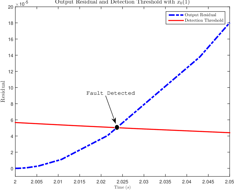
It can be deduced that yields divergent transient of because of the error steady state of with respect to certain initial conditions. Nevertheless, the steady states throughout cannot be said as the influence of . Fig. (2(d)), (2(e)), (2(f)) performs three different responses due to three various with disturbance observer. Compared to them, Fig. (2(g)), (2(h)), (2(i)) implement adaptive-Kalman showing slightly divergent outcome which are better than that of consensus filtering. Fig. (2(j)), (2(k)), and (2(l)) define the different fault detection where the output residual starts to overtake the threshold, meaning the fault is detected. From three , it results in , and respectively as the intersection between those two parameters, writing as . This can be summarized that the output residual would be relatively small for in comparison with the threshold. Due to the coincidence points after the transient observer, the time required to intersect the threshold is just slightly after the occurrence of the fault .
V Conclusion
The initial mathematical model of hydraulic system has been proposed along with the construction of stability properties. The estimation methods are applied with the Luenberger observer, adaptive-scaling Kalman, and consensus filtering to examine the unhealthy system. Fault detection scheme for certain time is designed and tested mathematically and in simulation. The results show that the fault detection scenarios are successfully proposed.




Acknowledgment
Thanks to Professor Thomas Parisini from the Imperial College London who has taught me in the lecture leading to finishing this paper and to LPDP (Indonesia Endowment Fund for Education) Scholarship from Indonesia.
References
- [1] Dingli Yu, D. N. Shields, and J. L. Mahtani, “A nonlinear fault detection method for a hydraulic system,” in 1994 International Conference on Control - Control ’94., vol. 2, March 1994, pp. 1318–1322 vol.2.
- [2] P. Bisták, “Identification and control of hydraulic system using visual feedback,” in 2016 International Conference on Emerging eLearning Technologies and Applications (ICETA), Nov 2016, pp. 29–34.
- [3] N. Helwig, S. Klein, and A. Schütze, “Identification and quantification of hydraulic system faults based on multivariate statistics using spectral vibration features,” Procedia Engineering, vol. 120, pp. 1225 – 1228, 2015, eurosensors 2015.
- [4] S. Vásquez, M. Kinnaert, and R. Pintelon, “Active fault diagnosis on a hydraulic pitch system based on frequency-domain identification,” IEEE Transactions on Control Systems Technology, vol. 27, no. 2, pp. 663–678, March 2019.
- [5] F. Wang and Y. Chen, “Dynamic characteristics of pressure compensator in underwater hydraulic system,” IEEE/ASME Transactions on Mechatronics, vol. 19, no. 2, pp. 777–787, April 2014.
- [6] S. Gayaka and B. Yao, “Fault detection, identification and accommodation for an electro-hydraulic system: An adaptive robust approach,” IFAC Proceedings Volumes, vol. 41, no. 2, pp. 13 815 – 13 820, 2008, 17th IFAC World Congress.
- [7] S. Sharifi, A. Tivay, S. M. Rezaei, M. Zareinejad, and B. Mollaei-Dariani, “Leakage fault detection in electro-hydraulic servo systems using a nonlinear representation learning approach,” ISA Transactions, vol. 73, pp. 154 – 164, 2018.
- [8] G. Shen, Z. Zhu, J. Zhao, W. Zhu, Y. Tang, and X. Li, “Real-time tracking control of electro-hydraulic force servo systems using offline feedback control and adaptive control,” ISA Transactions, vol. 67, pp. 356 – 370, 2017.
- [9] Z. MA, S. WANG, J. SHI, T. LI, and X. WANG, “Fault diagnosis of an intelligent hydraulic pump based on a nonlinear unknown input observer,” Chinese Journal of Aeronautics, vol. 31, no. 2, pp. 385 – 394, 2018.
- [10] K. Vereide, B. Svingen, T. K. Nielsen, and L. Lia, “The effect of surge tank throttling on governor stability, power control, and hydraulic transients in hydropower plants,” IEEE Transactions on Energy Conversion, vol. 32, no. 1, pp. 91–98, March 2017.
- [11] D. Angeli, “A lyapunov approach to incremental stability properties,” IEEE Transactions on Automatic Control, vol. 47, no. 3, pp. 410–421, March 2002.
- [12] D. Nesic and A. R. Teel, “Input-output stability properties of networked control systems,” IEEE Transactions on Automatic Control, vol. 49, no. 10, pp. 1650–1667, Oct 2004.
- [13] Y. Huang, Y. Zhang, B. Xu, Z. Wu, and J. A. Chambers, “A new adaptive extended kalman filter for cooperative localization,” IEEE Transactions on Aerospace and Electronic Systems, vol. 54, no. 1, pp. 353–368, Feb 2018.
- [14] V. Lippiello, B. Siciliano, and L. Villani, “Adaptive extended kalman filtering for visual motion estimation of 3d objects,” Control Engineering Practice, vol. 15, no. 1, pp. 123 – 134, 2007.
- [15] S. Roujol, B. Denis de Senneville, S. Hey, C. Moonen, and M. Ries, “Robust adaptive extended kalman filtering for real time mr-thermometry guided hifu interventions,” IEEE Transactions on Medical Imaging, vol. 31, no. 3, pp. 533–542, March 2012.
- [16] M. Efe, J. A. Bather, and D. P. Atherton, “An adaptive kalman filter with sequential rescaling of process noise,” in Proceedings of the 1999 American Control Conference (Cat. No. 99CH36251), vol. 6, June 1999, pp. 3913–3917 vol.6.
- [17] V. A. Bavdekar, R. B. Gopaluni, and S. L. Shah, “Evaluation of adaptive extended kalman filter algorithms for state estimation in presence of model-plant mismatch,” IFAC Proceedings Volumes, vol. 46, no. 32, pp. 184 – 189, 2013, 10th IFAC International Symposium on Dynamics and Control of Process Systems.
- [18] R. Olfati-Saber, “Distributed kalman filter with embedded consensus filters,” in Proceedings of the 44th IEEE Conference on Decision and Control, Dec 2005, pp. 8179–8184.
- [19] M. K. Wafi, “Filtering module on satellite tracking,” AIP Conference Proceedings, vol. 2088, no. 1, p. 020045, 2019.