System Identification on the Families of Auto-Regressive with Least-Square-Batch Algorithm

System identification, an error-correcting training scheme, is becoming more important dealing with either a system or process requiring to estimate the states with certain unknown variables. Further research even has modified from classic statistical method to regularisation considering the unhealthy matrix of minimization scheme [1], [2]. The idea of auto-regressive involves current and preceding data to be estimated with mutually independent per-sequence [3]. This model is then modified so as to obtain the best prediction, reducing the error. This is well-conducted by [4] proposing unknown number of epoch formula each sequence inducing the Markov process. Thanks to [5], the very early idea in predicting one-step ahead using either the median and the log-normal process of distribution. Moreover, the procedural modification applying Lasso scenario is also a choice as presented in [6]. This research is to examine basic properties from the family of auto-regressive along with the benefit of some iteration $N$ and batch $\kappa$. Beyond that, the assumptions of zero-mean and its counterpart along with either white and coloured noise are also considered.

The first and foremost is the stability properties of the system. The Lyapunov scenario as the most famed algorithm is proposed in this project [7]. While there has been a broad modification in determining the stability of the system, including strong passivity in nonlinear system as stated in [8], the mathematical foundation should be well-defined [9]. These basic information are then ready followed by some recursive or forecasting scheme with other bunch of methods. Least-square as prediction is to portray the best linear to show the data along with forecast the following data with respect to some instant time $t$, consisting the trend and the level of development. The more generalized with coloured noise system is presented in [10] referring to the original [11]. This paper comprises the problem formulation followed by the basic mathematical concepts. The next is the analytical result with three divergent scenarios ended by the numerical design and conclusion.

This paper presents the objectives of system identification:

1. 1.

   To elaborate the functions of expected value, variance, and covariance in a stationary process via static representation

2. 2.

   To describe mathematically the identification abilities of AR models of increasing order

3. 3.

   To compare the theoretical results with its simulation with empirical Least Square (LS) estimation

4. 4.

   To highlight the impact of coloured noises on the LS estimation

General design of the system model is presented in Fig. (1) defining that $P$ is the system plant along with $\xi$ as its parameter. $\nu$ comprises either fault $(f)$ or disturbances $(d)$ whilst $u$ and $z$ denote as the accessible input and the controlled variable in turn. The space of possible results is denoted by $\mathcal{S}$ and its single result of $s$ is $\in\mathcal{S}$ while the events of certain interest are defined as $s_{\epsilon}$ which is also the subset of $\mathcal{S}$. Furthermore, the patterns of the output depend on the parameters on algebraic equation of the system $P_{\xi}$ resulting its roots either real or complex. The common features of the dynamics constitute that the $(t)$ continuous or $(z)$ discrete-mathematical structure is built by differential equation and it has been a-priori knowledge being found from the physical properties of the system.

The applied random variable is a variable of $\mathcal{F}(s)$ obtaining values according to the result $s\in\mathcal{S}$ of a random trial through a function $\Theta(\bullet)$. The probability distribution function supplies the data on the random variable so that the equation of $F(x)=\mathcal{P}(v\leq x)$ can be denoted as,

meaning that $\mathcal{P}$ is the specific probability distribution being made of function $F$ with points between $a$ and $b$ while the probability density of $f^{\dagger}$ creating an area of $\mathcal{P}(v\in[a,b])$ is defined as follows,

Furthermore, the expected value E and its variance $\mathcal{Q}$ of a fault and disturbance are presented as,

with standard deviation of $\sigma(v)=\sqrt{\mathcal{Q}_{v}}$. Keep in mind that, given two variables of $v_{1}(s)$ and $v_{2}(s)$, the results of $v(s)$, $\textbf{E}(v)$, and $\mathcal{Q}_{v}$ are $v(s)=v_{1}(s)+v_{2}(s)$, $\textbf{E}(v)=\textbf{E}(v_{1})+\textbf{E}(v_{2})$, and

in turn, with $\mathcal{Q}_{v}=\textbf{E}\left\{[v-\textbf{E}(v)][v-\textbf{E}(v)]^{T}\right\}$. A Gaussian random variable exists if the average $\mu=\textbf{E}(v)$ and variance $\mathcal{Q}$ or $\sigma^{2}$ satisfies:

with respect to the properties of the $v$ in terms of correlation and independent, again, the two random variables $v_{1}$ and $v_{2}$ are uncorrelated if

whereas they are called as independent if

hence, the stochastic process originally requires the portrayal of probability distribution and is a collection of infinite random variable sequenced with respect to time. A stochastic process of $v(t)$ is called white being defined as $v\sim\mathcal{W}\mathcal{N}(0,\lambda^{2})$ if $\textbf{E}[v(t)]=0$ and

Beyond that, apart from examine the unbiased estimation, the minimization of the variance $\Phi$ could be tested. The estimator of $\bar{\theta}^{1}$ is better than that of $\bar{\theta}^{2}$ if $\Phi_{\bar{\theta}^{1}}\leq\Phi_{\bar{\theta}^{2}}$ or, if $\bar{\theta}^{i}$ is a vector, then $\Phi_{\bar{\theta}^{2}}-\Phi_{\bar{\theta}^{1}}\geq 0$. The asymptotic characteristic is affected by the number of simulated data $N$ which also influence the better estimation and reduce the uncertainty. Suppose three different variances $\Phi_{m}$ with the same expected value E such that $\textbf{E}[\bar{\theta}^{i}]=\theta$ with $i=1\to m$ and $m_{3}>m_{2}>m_{1}$, the estimate $\bar{\theta}^{m}$ is said good at converging to $\theta$ if

where $\bar{\theta}^{m},\theta$ and $\lVert\bar{\theta}^{m}-\theta\rVert$ are the random and constant vector along with a scalar random with good mean variable in turn.

This section acts as the numerical findings which are then compared to the simulations with Least Square algorithm being elaborated in the following section. There are three different scenarios. First is the basic with zero-mean and the second is to alter from zero-mean to non-zero mean yet the other conditions are kept the same and the following is to change the covariance instead of the mean.

Linear regression as typical context related to least-square estimator is initialized with $n+1$ variables of $y(t)$, $\theta_{1}(t),\dots,\theta_{n}(t)$ over an interval of $t=1,2,\dots,N$. It is then required, if possible, $n$ variables $\zeta_{1},\zeta_{2},\dots,\zeta_{n}$, such that

is denoted as linear regression according to $\theta(t)$ variable which is able to rewrite as a matrix function of $\zeta^{\top}\theta$ acting as row matrices. Recalling equation (11) with certain iteration of $N$ along with some random sequence of either independent, the recursive equation is set as,

While the appearance of error $\epsilon$ referring to $y(t)-\zeta^{\top}\theta$ is undeniable, to minimize it is a key by obtaining the optimal vector of $\theta^{\star}$. It can be achieved by the function of quadratic cost, therefore

such that after differentiating the cost function in terms of $\theta$-element generating the zero results, the $\theta$ could be determined by converting the equality of both row and column vectors. If sum of the product of $\zeta(t)\zeta(t)^{\top}$ from $1\to N$ is non-singular,

it can be deduced that for the minimum of $\Gamma$, $\lVert y_{N}-\zeta_{N}\theta\rVert$ should be orthogonal to $\zeta_{N}\theta$. This is due to the symmetric and positive semi-definite so that $\theta_{N}$ yields in local minimum of $\Gamma(\theta)$. Moreover, the sum of $\zeta(t)\zeta(t)^{\top}$ results in two divergent scenarios of determinant whether it is zero or not. Unique global minimum or identifiability is situated if it is not zero while for the counterpart result, $\theta_{N}$ is one among the infinite global minima. The least-square algorithm in Eq. (47) is then used to computed the optimal $\left[\theta_{1}^{\star},\theta_{2}^{\star}\right]$ of either families. The variation of $N$ is also applied to observe the effectiveness of the recursive. Furthermore, the $\kappa$ independent batches of the generated $\Pi_{i}$, such that

with certain $N$ is required to calculate the empirical mean for both families, such that

along with some variances as follows. The broader batches of $\check{\Pi}_{i}$ with certain constant $\alpha$, therefore $\alpha N$ is designed.

with,

The process $q(\bullet)$ is supposed to be coloured noise based on the following recursive equation,

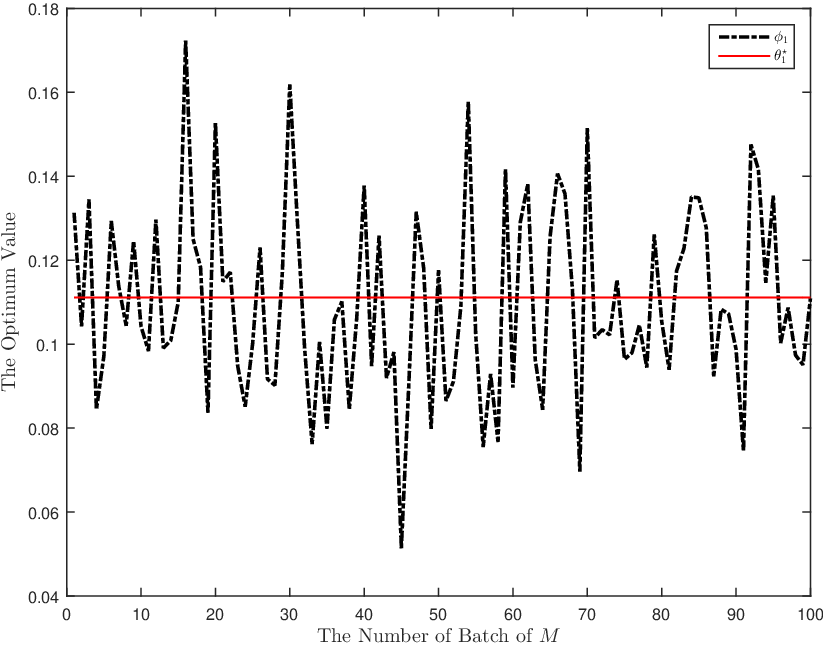
where $\eta\sim\mathcal{W}\mathcal{N}\left(0,1\right)$ and $\eta(\bullet)$ is independent from $v(\bullet)$. This scenario is then observed being compared to that of white noise in the preceding. It can be concluded that the variance $\Phi_{\theta_{2}}^{\star}$ is slightly smaller than that of $\Phi_{\theta_{1}}^{\star}$ meaning that the model approximation to the true system of AR(2) is better than that of AR(1). In terms of the simulation, the yields are closer to the hand-made calculation relative to certain $\alpha N,\alpha=1\to\infty$, the greater $\alpha$ results in better approximation of optimal value leading to the variance. With $\alpha=[1,2]$ and $N=1000$ in AR(1) for instance, it generates

optimal value $\theta_{1}^{\star}$ respectively compared to the hand calculation $0.11$ while as for AR(2) as $\theta_{2}^{\star}$ with the same design of $\alpha$, it yields $[\phi_{1},\phi_{2}]^{\top}$ as

in turn against the origin of $[0.108,0.025]^{\top}$. For certain $\kappa=100,N=1000$ and $\alpha=[1,2]$, the $\theta_{1}^{\star}$ AR(1) generates,

and these values of the estimated parameter is close to that of the optimal $\theta_{1}^{\star}=0.11$. This is due to the more data provided leading to better approximation. With respect to AR(2), the optimal parameter $\theta_{2}^{\star}$ and the variance $\Phi_{\theta_{2}}$ with the same scenarios of $\kappa,N,\alpha$ are obtained as follows,

for $N=1000$ whereas with $\alpha=2$, it gains

compared to the origin of $[\phi_{1},\phi_{2}]^{\top}=[0.1083,0.0250]^{\top}$. Moving to coloured noise which generates divergent approximation, for AR(1) with the same design as the white noise and hand-mad calculation, the optimal value $\theta_{1}^{\star}$ comprises,

This not surprising though, as for each sequence iteration, it yields a divergent stimulated data influencing the system so that it is far compared to that of the white. As for AR(2), $\theta_{2}^{\star}$ is reached as follows,

which show the same pattern as in AR(1). With respect to batches $\Pi_{i}\to\kappa$ scenario, the optimal value of AR(1) constitutes beyond the origin meaning that it is biased affecting the empirical and its variances, such that

and AR(2) is also performing the same another convergence number apart from the origin (hand-made calculation), it is proven as in the following,

for $N=1000$ whereas with $\alpha=2$, it gains

The mathematical scenarios of switching from zero-mean to non zero-mean along with from white to coloured have been studied to give better picture of the mathematical characteristic from either families. The simulation designs have been proposed in order to observe the effectiveness of certain number of recursive $N$ along with the batches concept $\kappa$ compared to the hand calculation of the optimal values. The greater number of $N$ and batches $\kappa$ with the more complex design of estimate AR(2) results in better approximation of the true system in terms of empirical mean and variance. Further research is to compare another more complex families with modified stochastic scenarios.

Thanks to Professor Thomas Parisini from the Imperial College London who has taught me in the lecture leading to finishing this paper and to LPDP (Indonesia Endowment Fund for Education) Scholarship from Indonesia.

References

• [1] L. Ljung, T. Chen, and B. Mu, “A shift in paradigm for system identification,” International Journal of Control, pp. 1–8, 2019.
• [2] J. Nagumo and A. Noda, “A learning method for system identification,” IEEE Transactions on Automatic Control, vol. 12, no. 3, pp. 282–287, June 1967.
• [3] E. G. Hurst, “Bayesian autoregressive time series analysis,” IEEE Transactions on Systems Science and Cybernetics, vol. 4, no. 3, pp. 317–324, Sep. 1968.
• [4] J. Ding, S. Shahrampour, K. Heal, and V. Tarokh, “Analysis of multistate autoregressive models,” IEEE Transactions on Signal Processing, vol. 66, no. 9, pp. 2429–2440, May 2018.
• [5] P. Stoica, “Prediction of autoregressive lognormal processes,” IEEE Transactions on Automatic Control, vol. 25, no. 2, pp. 292–293, April 1980.
• [6] Y. Nardi and A. Rinaldo, “Autoregressive process modeling via the lasso procedure,” Journal of Multivariate Analysis, vol. 102, no. 3, pp. 528 – 549, 2011.
• [7] R. K. Yedavalli, “Conditions for the existence of a common quadratic lyapunov function via stability analysis of matrix families,” in Proceedings of the 2002 American Control Conference (IEEE Cat. No.CH37301), vol. 2, May 2002, pp. 1296–1301 vol.2.
• [8] C. Yang, J. Sun, Q. Zhang, and X. Ma, “Lyapunov stability and strong passivity analysis for nonlinear descriptor systems,” IEEE Transactions on Circuits and Systems I: Regular Papers, vol. 60, no. 4, pp. 1003–1012, April 2013.
• [9] W. R. Melvin, “Stability properties of functional difference equations,” Journal of Mathematical Analysis and Applications, vol. 48, no. 3, pp. 749 – 763, 1974.
• [10] M. V. Dragosevic and S. S. Stankovic, “A generalized least squares method for frequency estimation,” IEEE Transactions on Acoustics, Speech, and Signal Processing, vol. 37, no. 6, pp. 805–819, June 1989.
• [11] M. Morf and T. Kailath, “Square-root algorithms for least-squares estimation,” IEEE Transactions on Automatic Control, vol. 20, no. 4, pp. 487–497, August 1975.
VII Appendices
Appendix A - y⁡(t)y(t)
ℋ=\displaystyle\mathcal{H}=\; 11−λ​z−1\displaystyle\frac{1}{1-\lambda z^{-1}}
Y⁡(z)=\displaystyle Y(z)=\; 𝒬⁡(z)​ℋ​(z)+𝒱⁡(z)\displaystyle\mathcal{Q}(z)\mathcal{H}(z)+\mathcal{V}(z)
Y⁡(z)+Y⁡(z)ℋ⁡(z)=\displaystyle Y(z)+\frac{Y(z)}{\mathcal{H}(z)}=\; Y⁡(z)+𝒬⁡(z)+𝒱⁡(z)ℋ⁡(z)\displaystyle Y(z)+\mathcal{Q}(z)+\frac{\mathcal{V}(z)}{\mathcal{H}(z)}
Y⁡(z)=\displaystyle Y(z)=\; Y⁡(z)−Y⁡(z)ℋ⁡(z)+𝒬⁡(z)+𝒱⁡(z)ℋ⁡(z)\displaystyle Y(z)-\frac{Y(z)}{\mathcal{H}(z)}+\mathcal{Q}(z)+\frac{\mathcal{V}(z)}{\mathcal{H}(z)}
=\displaystyle=\; Y⁡(z)​[1−1ℋ⁡(z)]+𝒬⁡(z)+𝒱⁡(z)ℋ⁡(z)\displaystyle Y(z)\left[1-\frac{1}{\mathcal{H}(z)}\right]+\mathcal{Q}(z)+\frac{\mathcal{V}(z)}{\mathcal{H}(z)}
=\displaystyle=\; Y⁡(z)​[λ​z−1]+𝒬⁡(z)+𝒱⁡(z)​[1−λ​z−1]\displaystyle Y(z)\left[\lambda z^{-1}\right]+\mathcal{Q}(z)+\mathcal{V}(z)\left[1-\lambda z^{-1}\right]
y⁡(t)=\displaystyle y(t)=\; λ​y​(t−1)+q⁡(t)+v⁡(t)−λ​v​(t−1)\displaystyle\lambda y(t-1)+q(t)+v(t)-\lambda v(t-1)
Appendix B - Expected Value Ey\textbf{E}_{y}
E​[y​(t)]=\displaystyle\textbf{E}[y(t)]=\; E​[λ​y​(t−1)+q⁡(t)+v⁡(t)−λ​v​(t−1)]\displaystyle\textbf{E}[\lambda y(t-1)+q(t)+v(t)-\lambda v(t-1)]
=\displaystyle=\; λ​E​[y⁡(t−1)]+E​[q⁡(t)]+E​[v⁡(t)]−λ​E​[v⁡(t−1)]\displaystyle\lambda\textbf{E}[y(t-1)]+\textbf{E}[q(t)]+\textbf{E}[v(t)]-\lambda\textbf{E}[v(t-1)]
=\displaystyle=\; λ​y¯+q¯+v¯−λ​v¯\displaystyle\lambda\bar{y}+\bar{q}+\bar{v}-\lambda\bar{v}
=\displaystyle=\; v¯+q¯1−λ\displaystyle\bar{v}+\dfrac{\bar{q}}{1-\lambda}
Appendix C - Variance Φy\Phi_{y}
Φy=\displaystyle\Phi_{y}=\; E​{[y⁡(t)−y¯]2}\displaystyle\textbf{E}\left\{[y(t)-\bar{y}]^{2}\right\}
=\displaystyle=\; E​[y​(t)2−2​y​(t)​y¯+y¯2]\displaystyle\textbf{E}\left[y(t)^{2}-2y(t)\bar{y}+\bar{y}^{2}\right]
=\displaystyle=\; E​[y​(t)2]−E​[y¯2]⟶E​[y¯2]=0\displaystyle\textbf{E}\left[y(t)^{2}\right]-\textbf{E}\left[\bar{y}^{2}\right]\longrightarrow\textbf{E}\left[\bar{y}^{2}\right]=0
=\displaystyle=\; E​{[λ​y​(t−1)+q⁡(t)⏟A+v⁡(t)−λ​v​(t−1)⏞B]2}\displaystyle\textbf{E}\left\{\left[\underbrace{\lambda y(t-1)+q(t)}_{A}+\overbrace{v(t)-\lambda v(t-1)}^{B}\right]^{2}\right\}
=\displaystyle=\; E​[A2+2​A​B+B2]\displaystyle\textbf{E}\left[A^{2}+2AB+B^{2}\right]
E​[A2]=\displaystyle\textbf{E}\left[A^{2}\right]=\; E​[λ2​y​(t−1)2+2​λ​y​(t−1)​q​(t)+q​(t)2]\displaystyle\textbf{E}\left[\lambda^{2}y(t-1)^{2}+2\lambda y(t-1)q(t)+q(t)^{2}\right]
=\displaystyle=\; E​[λ2​y​(t−1)2]+2​E​[λ​y​(t−1)​q​(t)]+E​[q​(t)2]\displaystyle\textbf{E}\left[\lambda^{2}y(t-1)^{2}\right]+2\textbf{E}\left[\lambda y(t-1)q(t)\right]+\textbf{E}\left[q(t)^{2}\right]
=\displaystyle=\; λ2​Φy+δ2\displaystyle\lambda^{2}\Phi_{y}+\delta^{2}
E​[2​A​B]=\displaystyle\textbf{E}\left[2AB\right]=\; 2E[λy(t−1)v(t)−λ2y(t−1)v(t−1)+q(t)v(t)\displaystyle 2\textbf{E}\left[\lambda y(t-1)v(t)-\lambda^{2}y(t-1)v(t-1)+q(t)v(t)\right.
−λq(t)v(t−1)]\displaystyle-\lambda q(t)v(t-1)]
=\displaystyle=\; 2​E​[λ​y​(t−1)​v​(t)]−2​λ2​E​[y⁡(t−1)​v​(t−1)]\displaystyle 2\textbf{E}\left[\lambda y(t-1)v(t)\right]-2\lambda^{2}\textbf{E}\left[y(t-1)v(t-1)\right]
+2​E​[q⁡(t)​v​(t)]−2​E​[λ​q​(t)​v​(t−1)]\displaystyle+2\textbf{E}\left[q(t)v(t)\right]-2\textbf{E}\left[\lambda q(t)v(t-1)\right]
=\displaystyle=\; −2​λ2​ξ2\displaystyle-2\lambda^{2}\xi^{2}
E​[B2]=\displaystyle\textbf{E}\left[B^{2}\right]=\; E​[v​(t)2−2​λ​v​(t)​v​(t−1)+λ2​v​(t−1)2]\displaystyle\textbf{E}\left[v(t)^{2}-2\lambda v(t)v(t-1)+\lambda^{2}v(t-1)^{2}\right]
=\displaystyle=\; E​[v​(t)2]−2​λ​E​[v⁡(t)​v​(t−1)]+λ2​E​[v​(t−1)2]\displaystyle\textbf{E}\left[v(t)^{2}\right]-2\lambda\textbf{E}\left[v(t)v(t-1)\right]+\lambda^{2}\textbf{E}\left[v(t-1)^{2}\right]
=\displaystyle=\; ξ2+λ2​ξ2\displaystyle\xi^{2}+\lambda^{2}\xi^{2}
Φy=\displaystyle\Phi_{y}=\; λ2​Φy+δ2−2​λ2​ξ2+ξ2+λ2​ξ2\displaystyle\lambda^{2}\Phi_{y}+\delta^{2}-2\lambda^{2}\xi^{2}+\xi^{2}+\lambda^{2}\xi^{2}
=\displaystyle=\; δ21−λ2+ξ2\displaystyle\frac{\delta^{2}}{1-\lambda^{2}}+\xi^{2}
Appendix D - Covariance Ψy\Psi_{y}
Ψy​(τ)=\displaystyle\Psi_{y}(\tau)=\; E{[y(t)−y¯][y(t−τ)−y¯]}⟶y¯=0\displaystyle\textbf{E}\Bigl\{\left[y(t)-\bar{y}\right]\left[y(t-\tau)-\bar{y}\right]\Bigl\}\longrightarrow\bar{y}=0
=\displaystyle=\; E{[ay(t−1)+e(t)+v(t)−av(t−1)][y(t−τ)]}\displaystyle\textbf{E}\Bigl\{\left[ay(t-1)+e(t)+v(t)-av(t-1)\right]\left[y(t-\tau)\right]\Bigl\}
=\displaystyle=\; λ​E​[y⁡(t−1)​y​(t−τ)]+E​[e⁡(t)​y​(t−τ)]\displaystyle\lambda\textbf{E}\left[y(t-1)y(t-\tau)\right]+\textbf{E}\left[e(t)y(t-\tau)\right]
+E​[v⁡(t)​y​(t−τ)]−λ​E​[v⁡(t−1)​y​(t−τ)]\displaystyle+\textbf{E}\left[v(t)y(t-\tau)\right]-\lambda\textbf{E}\left[v(t-1)y(t-\tau)\right]
Ψy​(0)=\displaystyle\Psi_{y}(0)=\; λ​Ψ​(1)+δ2+ξ2\displaystyle\lambda\Psi(1)+\delta^{2}+\xi^{2}
Ψy​(1)=\displaystyle\Psi_{y}(1)=\; λ​Ψ​(0)−λ​ξ2\displaystyle\lambda\Psi(0)-\lambda\xi^{2}
Ψy​(2)=\displaystyle\Psi_{y}(2)=\; λ​Ψ​(1)\displaystyle\lambda\Psi(1)
Appendix D⋆ - Covariance Ψy​(τ)⟶τ=0,1,2\Psi_{y}(\tau)\longrightarrow\tau=0,1,2
Ψy​(1)≔\displaystyle\Psi_{y}(1)\coloneqq\; Ψ⁡(1)λ+ξ2=λ​Ψ​(1)+δ2+ξ2\displaystyle\frac{\Psi(1)}{\lambda}+\xi^{2}=\lambda\Psi(1)+\delta^{2}+\xi^{2}
≔\displaystyle\coloneqq\; λ​δ21−λ2\displaystyle\frac{\lambda\delta^{2}}{1-\lambda^{2}}
Ψy​(0)≔\displaystyle\Psi_{y}(0)\coloneqq\; λ​λ​δ21−λ2+δ2+ξ2\displaystyle\lambda\frac{\lambda\delta^{2}}{1-\lambda^{2}}+\delta^{2}+\xi^{2}
≔\displaystyle\coloneqq\; δ21−λ2+ξ2⟶Φy\displaystyle\frac{\delta^{2}}{1-\lambda^{2}}+\xi^{2}\longrightarrow\Phi_{y}
Ψy​(2)≔\displaystyle\Psi_{y}(2)\coloneqq\; λ​Ψ​(1)\displaystyle\lambda\Psi(1)
≔\displaystyle\coloneqq\; λ2​δ21−λ2⟶λτ​δ21−λ2​ for ​Ψy​(τ>1)\displaystyle\frac{\lambda^{2}\delta^{2}}{1-\lambda^{2}}\longrightarrow\frac{\lambda^{\tau}\delta^{2}}{1-\lambda^{2}}\textrm{ for }\Psi_{y}(\tau>1)
Appendix E - Γ⁡(θ1)⟶ϕ1\Gamma(\theta_{1})\longrightarrow\phi_{1}
Γ⁡(θ1)=\displaystyle\Gamma(\theta_{1})=\; E​{[y⁡(t)−y^​(t|t−1)]2}\displaystyle\textbf{E}\left\{\left[y(t)-\hat{y}(t|t-1)\right]^{2}\right\}
=\displaystyle=\; E​{[y⁡(t)−ϕ1​y​(t−1)]2}\displaystyle\textbf{E}\left\{\left[y(t)-\phi_{1}y(t-1)\right]^{2}\right\}
=\displaystyle=\; E​[y​(t)2−2​ϕ1​y​(t)​y​(t−1)+ϕ12​y​(t−1)2]\displaystyle\textbf{E}\left[y(t)^{2}-2\phi_{1}y(t)y(t-1)+\phi^{2}_{1}y(t-1)^{2}\right]
=\displaystyle=\; Ψy​(0)−2​ϕ1​Ψy​(1)+ϕ12​Ψy​(0)\displaystyle\Psi_{y}(0)-2\phi_{1}\Psi_{y}(1)+\phi^{2}_{1}\Psi_{y}(0)
=\displaystyle=\; (1+ϕ12)​Ψy​(0)−2​ϕ1​Ψy​(1)\displaystyle\left(1+\phi^{2}_{1}\right)\Psi_{y}(0)-2\phi_{1}\Psi_{y}(1)
∂Γ⁡(θ1)∂ϕ1=\displaystyle\frac{\partial\Gamma(\theta_{1})}{\partial\phi_{1}}=\; 2​ϕ1​Ψy​(0)−2​Ψy​(1)=0\displaystyle 2\phi_{1}\Psi_{y}(0)-2\Psi_{y}(1)=0
ϕ1=\displaystyle\phi_{1}=\; Ψy​(1)Ψy​(0)⟶λ​Ψy​(0)−λ​ξ2Ψy​(0)\displaystyle\frac{\Psi_{y}(1)}{\Psi_{y}(0)}\longrightarrow\frac{\lambda\Psi_{y}(0)-\lambda\xi^{2}}{\Psi_{y}(0)}
=\displaystyle=\; λ​δ2δ2+(1−λ2)​ξ2\displaystyle\frac{\lambda\delta^{2}}{\delta^{2}+(1-\lambda^{2})\xi^{2}}
Appendix F - Γ⁡(θ2)⟶θ2⋆≔[ϕ1,ϕ2]⊤\Gamma(\theta_{2})\longrightarrow\theta_{2}^{\star}\coloneqq\left[\phi_{1},\phi_{2}\right]^{\top}
Γ⁡(θ2)=\displaystyle\Gamma(\theta_{2})=\; E​{[y⁡(t)−y^​(t|t−1)]2}\displaystyle\textbf{E}\left\{\left[y(t)-\hat{y}(t|t-1)\right]^{2}\right\}
=\displaystyle=\; E​{[y⁡(t)−ϕ1​y​(t−1)−ϕ2​y​(t−2)]2}\displaystyle\textbf{E}\left\{\left[y(t)-\phi_{1}y(t-1)-\phi_{2}y(t-2)\right]^{2}\right\}
=\displaystyle=\; E[y(t)2+ϕ12y(t−1)2+ϕ22y(t−2)2\displaystyle\textbf{E}\left[y(t)^{2}+\phi^{2}_{1}y(t-1)^{2}+\phi^{2}_{2}y(t-2)^{2}\right.
−2​ϕ1​y​(t)​y​(t−1)−2​ϕ2​y​(t)​y​(t−2)\displaystyle-2\phi_{1}y(t)y(t-1)-2\phi_{2}y(t)y(t-2)
+2ϕ1ϕ2y(t−1)y(t−2)]\displaystyle+2\phi_{1}\phi_{2}y(t-1)y(t-2)]
=\displaystyle=\; Ψy​(0)+ϕ12​Ψy​(0)+ϕ22​Ψy​(0)−2​ϕ1​Ψy​(1)\displaystyle\Psi_{y}(0)+\phi_{1}^{2}\Psi_{y}(0)+\phi_{2}^{2}\Psi_{y}(0)-2\phi_{1}\Psi_{y}(1)
−2​ϕ2​Ψy​(2)+2​ϕ1​ϕ2​Ψy​(1)\displaystyle-2\phi_{2}\Psi_{y}(2)+2\phi_{1}\phi_{2}\Psi_{y}(1)
=\displaystyle=\; (1+ϕ12+ϕ22)​Ψy​(0)+2​ϕ1​(ϕ2−1)​Ψy​(1)\displaystyle\left(1+\phi^{2}_{1}+\phi^{2}_{2}\right)\Psi_{y}(0)+2\phi_{1}\left(\phi_{2}-1\right)\Psi_{y}(1)
−2​ϕ2​Ψy​(2)\displaystyle-2\phi_{2}\Psi_{y}(2)
∂Γ⁡(θ2)∂ϕ1=\displaystyle\frac{\partial\Gamma(\theta_{2})}{\partial\phi_{1}}=\; 2​ϕ1​Ψy​(0)+2​ϕ2​Ψy​(1)−2​Ψy​(1)=0\displaystyle 2\phi_{1}\Psi_{y}(0)+2\phi_{2}\Psi_{y}(1)-2\Psi_{y}(1)=0
ϕ1=\displaystyle\phi_{1}=\; Ψy​(1)−ϕ2​Ψy​(1)Ψy​(0)\displaystyle\frac{\Psi_{y}(1)-\phi_{2}\Psi_{y}(1)}{\Psi_{y}(0)}
=\displaystyle=\; Ψy​(1)−(Ψy​(2)​Ψy​(0)−Ψy​(1)2Ψy​(0)2−Ψy​(1)2)​Ψy​(1)Ψy​(0)\displaystyle\frac{\Psi_{y}(1)-\left(\dfrac{\Psi_{y}(2)\Psi_{y}(0)-\Psi_{y}(1)^{2}}{\Psi_{y}(0)^{2}-\Psi_{y}(1)^{2}}\right)\Psi_{y}(1)}{\Psi_{y}(0)}
=\displaystyle=\; Ψy​(1)​Ψy​(0)−Ψy​(2)​Ψy​(1)Ψy​(0)2−Ψy​(1)2\displaystyle\frac{\Psi_{y}(1)\Psi_{y}(0)-\Psi_{y}(2)\Psi_{y}(1)}{\Psi_{y}(0)^{2}-\Psi_{y}(1)^{2}}
=\displaystyle=\; λ​δ2​(δ2+ξ2)(δ2+ξ2)2−λ2​ξ4\displaystyle\frac{\lambda\delta^{2}\left(\delta^{2}+\xi^{2}\right)}{\left(\delta^{2}+\xi^{2}\right)^{2}-\lambda^{2}\xi^{4}}
∂Γ⁡(θ2)∂ϕ1=\displaystyle\frac{\partial\Gamma(\theta_{2})}{\partial\phi_{1}}=\; 2​ϕ2​Ψy​(0)+2​ϕ1​Ψy​(1)−2​Ψy​(2)=0\displaystyle 2\phi_{2}\Psi_{y}(0)+2\phi_{1}\Psi_{y}(1)-2\Psi_{y}(2)=0
ϕ2=\displaystyle\phi_{2}=\; Ψy​(2)−ϕ1​Ψy​(1)Ψy​(0)\displaystyle\frac{\Psi_{y}(2)-\phi_{1}\Psi_{y}(1)}{\Psi_{y}(0)}
=\displaystyle=\; Ψy​(2)−(Ψy​(1)​Ψy​(0)−Ψy​(2)​Ψy​(1)Ψy​(0)2−Ψy​(1)2)​Ψy​(1)Ψy​(0)\displaystyle\frac{\Psi_{y}(2)-\left(\dfrac{\Psi_{y}(1)\Psi_{y}(0)-\Psi_{y}(2)\Psi_{y}(1)}{\Psi_{y}(0)^{2}-\Psi_{y}(1)^{2}}\right)\Psi_{y}(1)}{\Psi_{y}(0)}
=\displaystyle=\; Ψy​(2)​Ψy​(0)−Ψy​(1)2Ψy​(0)2−Ψy​(1)2\displaystyle\frac{\Psi_{y}(2)\Psi_{y}(0)-\Psi_{y}(1)^{2}}{\Psi_{y}(0)^{2}-\Psi_{y}(1)^{2}}
=\displaystyle=\; λ2​δ2​ξ2(δ2+ξ2)2−λ2​ξ4\displaystyle\frac{\lambda^{2}\delta^{2}\xi^{2}}{\left(\delta^{2}+\xi^{2}\right)^{2}-\lambda^{2}\xi^{4}}
Appendix G - Φθ1⋆\Phi_{\theta_{1}^{\star}} and Φθ2⋆\Phi_{\theta_{2}^{\star}}
Φθ1⋆=\displaystyle\Phi_{\theta_{1}^{\star}}=\; Γ⁡(θ1)=E​{[εθ1​(t)−ε¯θ1]2}⟶ε¯θ1=0\displaystyle\Gamma(\theta_{1})=\textbf{E}\left\{\left[\varepsilon_{\theta_{1}}(t)-\bar{\varepsilon}_{\theta_{1}}\right]^{2}\right\}\longrightarrow\bar{\varepsilon}_{\theta_{1}}=0
=\displaystyle=\; [1+ϕ12]​Ψy​(0)−2​ϕ1​Ψy​(1)⟶ϕ1​ from Eq. (21)\displaystyle\left[1+\phi_{1}^{2}\right]\Psi_{y}(0)-2\phi_{1}\Psi_{y}(1)\longrightarrow\phi_{1}\textrm{ from Eq. (21)}
=\displaystyle=\; [1+(λ​δ2δ2+(1−λ2)​ξ2)2]​δ2+(1−λ2)​ξ21−λ2\displaystyle\left[1+\left(\frac{\lambda\delta^{2}}{\delta^{2}+(1-\lambda^{2})\xi^{2}}\right)^{2}\right]\frac{\delta^{2}+(1-\lambda^{2})\xi^{2}}{1-\lambda^{2}}
−2​(λ​δ2δ2+(1−λ2)​ξ2)​λ​δ21−λ2\displaystyle-2\left(\frac{\lambda\delta^{2}}{\delta^{2}+(1-\lambda^{2})\xi^{2}}\right)\frac{\lambda\delta^{2}}{1-\lambda^{2}}
=\displaystyle=\; [δ2+(1−λ2)​ξ2]2−λ2​δ4[δ2+(1−λ2)​ξ2]​[1−λ2]\displaystyle\frac{\left[\delta^{2}+\left(1-\lambda^{2}\right)\xi^{2}\right]^{2}-\lambda^{2}\delta^{4}}{\left[\delta^{2}+\left(1-\lambda^{2}\right)\xi^{2}\right]\left[1-\lambda^{2}\right]}
=\displaystyle=\; δ4​(1−λ2)+2​δ2​ξ2​(1−λ2)+ξ4​(1−λ2)2[δ2+(1−λ2)​ξ2]​[1−λ2]\displaystyle\frac{\delta^{4}\left(1-\lambda^{2}\right)+2\delta^{2}\xi^{2}\left(1-\lambda^{2}\right)+\xi^{4}\left(1-\lambda^{2}\right)^{2}}{\left[\delta^{2}+\left(1-\lambda^{2}\right)\xi^{2}\right]\left[1-\lambda^{2}\right]}
=\displaystyle=\; (δ2+ξ2)2−λ2​ξ4δ2+(1−λ2)​ξ2\displaystyle\frac{\left(\delta^{2}+\xi^{2}\right)^{2}-\lambda^{2}\xi^{4}}{\delta^{2}+\left(1-\lambda^{2}\right)\xi^{2}}
Φθ2⋆=\displaystyle\Phi_{\theta_{2}^{\star}}=\; Γ⁡(θ2)=E​{[εθ2​(t)−ε¯θ2]2}⟶ε¯θ2=0\displaystyle\Gamma(\theta_{2})=\textbf{E}\left\{\left[\varepsilon_{\theta_{2}}(t)-\bar{\varepsilon}_{\theta_{2}}\right]^{2}\right\}\longrightarrow\bar{\varepsilon}_{\theta_{2}}=0
=\displaystyle=\; [1+ϕ12+ϕ22]​Ψy​(0)−[2​ϕ1−2​ϕ1​ϕ2]​Ψy​(1)\displaystyle\left[1+\phi_{1}^{2}+\phi_{2}^{2}\right]\Psi_{y}(0)-\left[2\phi_{1}-2\phi_{1}\phi_{2}\right]\Psi_{y}(1)
−2​ϕ2​Ψy​(2)⟶[ϕ1,ϕ2]​ from Eq. (22)\displaystyle-2\phi_{2}\Psi_{y}(2)\longrightarrow[\phi_{1},\phi_{2}]\textrm{ from Eq. (22)}
=\displaystyle=\; Ψy​(0)3−Ψy​(2)2​Ψy​(0)−2​Ψy​(1)2​Ψy​(0)\displaystyle\Psi_{y}(0)^{3}-\Psi_{y}(2)^{2}\Psi_{y}(0)-2\Psi_{y}(1)^{2}\Psi_{y}(0)
+2​Ψy​(1)2​Ψy​(2)⟶after some complex-algebra\displaystyle+2\Psi_{y}(1)^{2}\Psi_{y}(2)\longrightarrow\textrm{after some complex-algebra}
=\displaystyle=\; (δ2+(1−λ2)​ξ21−λ2)3−(λ2​δ21−λ2)2​δ2+(1−λ2)​ξ21−λ2\displaystyle\left(\frac{\delta^{2}+(1-\lambda^{2})\xi^{2}}{1-\lambda^{2}}\right)^{3}-\left(\frac{\lambda^{2}\delta^{2}}{1-\lambda^{2}}\right)^{2}\frac{\delta^{2}+(1-\lambda^{2})\xi^{2}}{1-\lambda^{2}}
−2​(λ​δ21−λ2)2​δ2+(1−λ2)​ξ21−λ2+2​λ​(λ​δ21−λ2)3\displaystyle-2\left(\frac{\lambda\delta^{2}}{1-\lambda^{2}}\right)^{2}\frac{\delta^{2}+(1-\lambda^{2})\xi^{2}}{1-\lambda^{2}}+2\lambda\left(\frac{\lambda\delta^{2}}{1-\lambda^{2}}\right)^{3}
=\displaystyle=\; (δ2+ξ2)3−λ2​(δ2​ξ+ξ3)2+2​λ​δ4​ξ21−λ2\displaystyle\frac{\left(\delta^{2}+\xi^{2}\right)^{3}-\lambda^{2}\left(\delta^{2}\xi+\xi^{3}\right)^{2}+2\lambda\delta^{4}\xi^{2}}{1-\lambda^{2}}
Appendix H - Γ⁡(θ1)⟶ϕ1\Gamma(\theta_{1})\longrightarrow\phi_{1}; (non) zero-mean
Γ⁡(θ1)=\displaystyle\Gamma(\theta_{1})=\; E​[y​(t)2−2​y​(t)​y​(t|t−1)+y​(t|t−1)2]\displaystyle\textbf{E}\left[y(t)^{2}-2y(t)y(t|t-1)+y(t|t-1)^{2}\right]
=\displaystyle=\; E{[yˇ(t)+y¯]2}−2ϕ1E{[yˇ(t)+y¯][yˇ(t−1)+y¯]}\displaystyle\textbf{E}\left\{\left[\check{y}(t)+\bar{y}\right]^{2}\right\}-2\phi_{1}\textbf{E}\Bigl\{\left[\check{y}(t)+\bar{y}\right]\left[\check{y}(t-1)+\bar{y}\right]\Bigl\}
+ϕ12​E​{[yˇ​(t−1)+y¯]2}\displaystyle+\phi_{1}^{2}\textbf{E}\left\{\left[\check{y}(t-1)+\bar{y}\right]^{2}\right\}
=\displaystyle=\; [1+ϕ12]​Ψy​(0)−2​ϕ1​Ψy​(1)+(1−ϕ1)2​y¯2\displaystyle\left[1+\phi_{1}^{2}\right]\Psi_{y}(0)-2\phi_{1}\Psi_{y}(1)+\left(1-\phi_{1}\right)^{2}\bar{y}^{2}
∂Γ⁡(θ1)∂ϕ1=\displaystyle\frac{\partial\Gamma(\theta_{1})}{\partial\phi_{1}}=\; −2​Ψy​(1)+2​ϕ1​Ψy​(0)−2​(1−ϕ1)​y¯2=0\displaystyle-2\Psi_{y}(1)+2\phi_{1}\Psi_{y}(0)-2\left(1-\phi_{1}\right)\bar{y}^{2}=0
θ1⋆≔\displaystyle\theta^{\star}_{1}\coloneqq\; Ψ⁡(1)+y¯2Ψ⁡(0)+y¯2\displaystyle\frac{\Psi(1)+\bar{y}^{2}}{\Psi(0)+\bar{y}^{2}}
Appendix I - Γ⁡(θ2)⟶θ2⋆≔[ϕ1,ϕ2]⊤\Gamma(\theta_{2})\longrightarrow\theta_{2}^{\star}\coloneqq\left[\phi_{1},\phi_{2}\right]^{\top}; (non) zero-mean
Γ⁡(θ2)=\displaystyle\Gamma(\theta_{2})=\; E​[y​(t)2−2​y​(t)​y​(t|t−1)+y​(t|t−1)2]\displaystyle\textbf{E}\left[y(t)^{2}-2y(t)y(t|t-1)+y(t|t-1)^{2}\right]
=\displaystyle=\; E{[yˇ(t)+y¯]2}−2E{[yˇ(t)+y¯][ϕ1yˇ(t−1)\displaystyle\textbf{E}\left\{\left[\check{y}(t)+\bar{y}\right]^{2}\right\}-2\textbf{E}\Bigl\{\left[\check{y}(t)+\bar{y}\right]\left[\phi_{1}\check{y}(t-1)\right.\Bigl.
+ϕ2yˇ(t−2)+(ϕ1+ϕ2)y¯]}+ϕ12E{[yˇ(t−1)]2}\displaystyle+\Bigl.\left.\phi_{2}\check{y}(t-2)+\left(\phi_{1}+\phi_{2}\right)\bar{y}\right]\Bigl\}+\phi_{1}^{2}\textbf{E}\left\{\left[\check{y}(t-1)\right]^{2}\right\}
+ϕ22​E​{[yˇ​(t−2)]2}+(ϕ1+ϕ2)​E​{[y¯]2}\displaystyle+\phi_{2}^{2}\textbf{E}\left\{\left[\check{y}(t-2)\right]^{2}\right\}+\left(\phi_{1}+\phi_{2}\right)\textbf{E}\left\{\left[\bar{y}\right]^{2}\right\}
+2​ϕ1​(ϕ1+ϕ2)​E​{[yˇ​(t−1)​y¯]}\displaystyle+2\phi_{1}\left(\phi_{1}+\phi_{2}\right)\textbf{E}\left\{\left[\check{y}(t-1)\bar{y}\right]\right\}
+2​ϕ2​(ϕ1+ϕ2)​E​{[yˇ​(t−2)​y¯]}\displaystyle+2\phi_{2}\left(\phi_{1}+\phi_{2}\right)\textbf{E}\left\{\left[\check{y}(t-2)\bar{y}\right]\right\}
+2​ϕ1​ϕ2​E​{[yˇ​(t−1)​yˇ​(t−2)]}\displaystyle+2\phi_{1}\phi_{2}\textbf{E}\left\{\left[\check{y}(t-1)\check{y}(t-2)\right]\right\}
−2​ϕ2​Ψy​(2)+2​ϕ1​ϕ2​Ψy​(1)+[1−(ϕ1+ϕ2)]2​y¯2\displaystyle-2\phi_{2}\Psi_{y}(2)+2\phi_{1}\phi_{2}\Psi_{y}(1)+\left[1-\left(\phi_{1}+\phi_{2}\right)\right]^{2}\bar{y}^{2}
∂Γ⁡(θ2)∂ϕ1=\displaystyle\frac{\partial\Gamma(\theta_{2})}{\partial\phi_{1}}=\; 0​ and ​∂Γ⁡(θ2)∂ϕ2= 0\displaystyle 0\textrm{ and }\frac{\partial\Gamma(\theta_{2})}{\partial\phi_{2}}=\;0
after some complex-algebra
ϕ1=\displaystyle\phi_{1}=\; Ψy​(1)​Ψy​(0)−Ψy​(2)​Ψy​(1)+y¯2​[Ψ⁡(0)−Ψ⁡(2)]Ψy​(0)2−Ψy​(1)2+2​y¯2​[Ψ⁡(0)−Ψ⁡(1)]\displaystyle\dfrac{\Psi_{y}(1)\Psi_{y}(0)-\Psi_{y}(2)\Psi_{y}(1)+\bar{y}^{2}\left[\Psi(0)-\Psi(2)\right]}{\Psi_{y}(0)^{2}-\Psi_{y}(1)^{2}+2\bar{y}^{2}\left[\Psi(0)-\Psi(1)\right]}
ϕ2=\displaystyle\phi_{2}=\; Ψy​(2)​Ψy​(0)−Ψy​(1)2+y¯2​[Ψ⁡(0)−2​Ψ​(1)+Ψ⁡(2)]Ψy​(0)2−Ψy​(1)2+2​y¯2​[Ψ⁡(0)−Ψ⁡(1)]\displaystyle\dfrac{\Psi_{y}(2)\Psi_{y}(0)-\Psi_{y}(1)^{2}+\bar{y}^{2}\left[\Psi(0)-2\Psi(1)+\Psi(2)\right]}{\Psi_{y}(0)^{2}-\Psi_{y}(1)^{2}+2\bar{y}^{2}\left[\Psi(0)-\Psi(1)\right]}
Appendix J - Φθ1⋆\Phi_{\theta_{1}^{\star}} and Φθ2⋆\Phi_{\theta_{2}^{\star}}; (non) zero-mean
ε¯θ1=\displaystyle\bar{\varepsilon}_{\theta_{1}}=\; E​[yˇ​(t)]+E​[y¯]−ϕ1​E​[yˇ​(t−1)]−ϕ1​E​[y¯]\displaystyle\textbf{E}\left[\check{y}(t)\right]+\textbf{E}\left[\bar{y}\right]-\phi_{1}\textbf{E}\left[\check{y}(t-1)\right]-\phi_{1}\textbf{E}\left[\bar{y}\right]
=\displaystyle=\; (1−ϕ1)​y¯\displaystyle(1-\phi_{1})\bar{y}
Φθ1⋆=\displaystyle\Phi_{\theta_{1}^{\star}}=\; Γ⁡(θ1)=E​{[εθ1​(t)−ε¯θ1]2}\displaystyle\Gamma(\theta_{1})=\textbf{E}\left\{\left[\varepsilon_{\theta_{1}}(t)-\bar{\varepsilon}_{\theta_{1}}\right]^{2}\right\}
=\displaystyle=\; E​{[yˇ​(t)+y¯−ϕ1​yˇ​(t−1)−ϕ1​y¯−(1−ϕ1)​y¯]2}\displaystyle\textbf{E}\left\{\left[\check{y}(t)+\bar{y}-\phi_{1}\check{y}(t-1)-\phi_{1}\bar{y}-\left(1-\phi_{1}\right)\bar{y}\right]^{2}\right\}
=\displaystyle=\; E​{[yˇ​(t)−ϕ1​yˇ​(t−1)]2}⟶Appendix E\displaystyle\textbf{E}\left\{\left[\check{y}(t)-\phi_{1}\check{y}(t-1)\right]^{2}\right\}\longrightarrow\textrm{{Appendix E}}
=\displaystyle=\; (δ2+ξ2)2−λ2​ξ4δ2+(1−λ2)​ξ2⟶Appendix G\displaystyle\frac{\left(\delta^{2}+\xi^{2}\right)^{2}-\lambda^{2}\xi^{4}}{\delta^{2}+\left(1-\lambda^{2}\right)\xi^{2}}\longrightarrow\textrm{{Appendix G}}
ε¯θ2=\displaystyle\bar{\varepsilon}_{\theta_{2}}=\; E​[yˇ​(t)]+E​[y¯]−ϕ1​E​[yˇ​(t−1)]−ϕ2​E​[yˇ​(t−2)]\displaystyle\textbf{E}\left[\check{y}(t)\right]+\textbf{E}\left[\bar{y}\right]-\phi_{1}\textbf{E}\left[\check{y}(t-1)\right]-\phi_{2}\textbf{E}\left[\check{y}(t-2)\right]
−(ϕ1+ϕ2)​E​[y¯]\displaystyle-\left(\phi_{1}+\phi_{2}\right)\textbf{E}\left[\bar{y}\right]
=\displaystyle=\; (1−ϕ1−ϕ2)​y¯\displaystyle(1-\phi_{1}-\phi_{2})\bar{y}
Φθ2⋆=\displaystyle\Phi_{\theta_{2}^{\star}}=\; Γ⁡(θ2)=E​{[εθ2​(t)−ε¯θ2]2}\displaystyle\Gamma(\theta_{2})=\textbf{E}\left\{\left[\varepsilon_{\theta_{2}}(t)-\bar{\varepsilon}_{\theta_{2}}\right]^{2}\right\}
=\displaystyle=\; E{[yˇ(t)+y¯−ϕ1yˇ(t−1)−ϕ2yˇ(t−2)\displaystyle\textbf{E}\Bigl\{\left[\check{y}(t)+\bar{y}-\phi_{1}\check{y}(t-1)-\phi_{2}\check{y}(t-2)\right.\Bigl.
−(ϕ1+ϕ2)y¯−(1−ϕ1−ϕ2)y¯]2}\displaystyle\Bigl.\left.-\left(\phi_{1}+\phi_{2}\right)\bar{y}-\left(1-\phi_{1}-\phi_{2}\right)\bar{y}\right]^{2}\Bigl\}
=\displaystyle=\; E​{[yˇ​(t)−ϕ1​yˇ​(t−1)−ϕ2​yˇ​(t−2)]2}\displaystyle\textbf{E}\left\{\left[\check{y}(t)-\phi_{1}\check{y}(t-1)-\phi_{2}\check{y}(t-2)\right]^{2}\right\}
Authors
First and Correspondence Author - Moh Kamalul Wafi was graduated from the Imperial College London majoring Control Systems under Department of Electrical and Electronics Engineering. I am currently with the Laboratory of Embedded and Cyber-Physical Systems, Department of Engineering Physics, Institut Teknologi Sepuluh Nopember, 60111, Indonesia