Abstract
Abstract This chapter is devoted to discussing the integration of intelligent reflecting surfaces (IRSs), or intelligent walls, in optical wireless communication (OWC) systems. IRS technology is a revolutionary concept that enables communication systems to harness the surrounding environment to control the propagation of light signals. Based on this, specific key performance indicators could be achieved by altering the electromagnetic response of the IRSs. In the following, we discuss the background theory and applications of IRSs and present a case study for an IRS-assisted indoor light-fidelity (LiFi) system. We then highlight some of the challenges related to this emerging concept and elaborate on future research directions.
Chapter 1 Optical Wireless Communications Using Intelligent Walls
Keywords: Intelligent Reflecting Surfaces (IRS), Optical Wireless Communications (OWC), light-fidelity (LiFi), Monte-Carlo Ray Tracing (MCRT), channel modelling
1.1 Introduction
The current surge in the number of mobile devices and the emerging internet-of-things (IoT) and internet-of-everything (IoE) applications are posing an unprecedented demand on wireless connectivity [6770233]. Mobile device density in service areas is approaching the region of more than one wireless device per square meter, which indicates that enhancing the capacity of wireless networks will become even more crucial in the foreseeable future. The use of conventional radio frequency (RF) small cells in such dense deployments proves challenging due to severe inter-cell co-channel interference (CCI). This is mainly attributed to the fact that RF signals travel beyond the cell boundaries. Moreover, there is a general consensus that the limited RF spectrum resources are not sufficient to future-proof wireless communications. Therefore, other parts of the electromagnetic (EM) spectrum have been explored for wireless connectivity. Particularly, optical wireless communications (OWC) presents a promising solution to satisfy the demands of future wireless networks. The main advantages offered by OWC are the freely available resources in the optical band of the EM spectrum which is in tera Hertz, with the visible light band alone being almost 2,600 times larger than the full RF spectrum [hycvppai2001]. Utilising the entire optical spectrum is not practically feasible due to the limitations of the transceivers front-ends and the necessary electro-optical (EO) and opto-electrical (OE) conversions. However, advancements in solid-state lighting and semiconductor devices are continuously leading to better capabilities, which means higher electrical bandwidth and narrower spectral emissions.
OWC technologies include free space optical communication (FSO) communication, ultraviolet (UV) communication, optical camera communication (OCC), visible light communications (VLC) and light-fidelity (LiFi). FSO communication systems provide point-to-point links over relatively large transmission distances and are mainly used for enabling low-cost wireless backhaul links indoors and outdoors. UV communication systems provide long-distance non-line-of-sight (NLoS) wireless connectivity through atmospheric scattering. UV links are robust to link blockage and, thus, do not require perfect alignment between the transmitter and the receiver. OCC utilizes cameras as receivers and operates in the visible light spectrum. OCC provides connectivity for low-rate, short-range line-of-sight (LoS) applications. VLC also utilizes visible light for wireless connectivity by employing a photo-diode (PD) as a receiver and offers high-speed, short-range LoS connectivity. The term LiFi refers to a network solution that utilizes wireless optical links, mainly VLC and infra-red (IR), to provide bidirectional connectivity with mobility support and seamless coverage.
LiFi arises as a promising solution to add a new dimension to spectrum heterogeneity in future wireless networks [7360112, HAAS2020443]. A LiFi network constitutes multiple interconnected short-range optical access points (APs), referred to as attocells. Each attocell serves a small number of users within a coverage area of a few square meters. The high directionality of light signals in LiFi networks allow for extreme cell densification and, hence, provide an effective solution to wireless coverage, and thus ultra-high capacity, in extremely dense deployments.
LiFi is envisioned to play a significant role in future cellular networks and IoT applications, including smart healthcare provisioning, smart infrastructure management, high-precision manufacturing, self-driven vehicles and remote robots operations, to count a few. These applications rely on smart autonomous operations and reliable high-speed connectivity that facilitate real-time interactions between different entities. Until recently, enhancing the communication capabilities of LiFi systems was primarily focused on the development of transmission and reception capabilities in the face of undesirable uncontrollable channel conditions. However, breakthrough advancements in programmable meta-surfaces resulted in a paradigm shift in the way wireless signal propagation is dealt with: from fully uncontrollable to tunable and customized wireless channel engineering. The recent rise of revolutionary intelligent reconfigurable surfaces (IRS) technology means that the environment itself can be programmed in order to enhance the performance of wireless communication systems. This enhancement comes in terms of spectral efficiency, energy efficiency, link reliability and security. Specifically, an intelligent surface constitutes a number of meta-surfaces that are artificially engineered in order to allow full manipulation of the incident EM waves. The EM response of these meta-surfaces can be altered on a macroscopic level to control the amplitude and phase of the incident beams. Based on this, it is possible to effectively control wireless signals to achieve the desired performance gains.
This chapter discusses the use of IRS or “intelligent walls” in the context of LiFi systems. Specifically, we discuss the background of this emerging technology and present some of its applications in Section 1.2. A case study for high-performance IRS-enabled LiFi systems is presented in Section 1.3, while Section 1.4 discusses some of the related challenges and future research directions.
1.2 Optical IRS: Background & Applications
In this section, we provide a comprehensive literature review of the integration of IRSs in OWC and shed light on the different applications of this emerging concept.
1.2.1 IRS from the Physics Perspective
The EM response of a surface is typically determined by the material it is made of as well as its geometry. Surface reflection behaviour can be classified into one of three responses: specular, diffuse, or glossy. Perfectly smooth surfaces act as mirrors and reflect light in a specular manner according to Snell’s law of reflection. Rough surfaces, on the other hand, scatter the incident light in all directions. Surfaces with a glossy nature reflect light in a way that contains both specular and diffuse components.
The term IRS refers to a surface containing an array of periodically arranged metasurface elements that are engineered to produce a controlled response to impinging light signals. The EM response of each element of the IRS array can be adjusted by tuning the surface impedance through electrical voltage stimulation, which can be controlled via field-programmable gate array (FPGA) chips. Various IRS designs have been presented in the literature using different numbers of layers as well as different materials, including liquid crystal, meta-lenses with artificial muscles, doped semiconductors and electromechanical switches. The fundamental architecture of an IRS is depicted in Fig. 1.1. Since the physical layer characteristics of IRSs can be controlled by software, they are also termed software-defined surfaces (SDSs). Although the use of metasurfaces in OWC have only recently became an active area of research, their capabilities in light manipulation have already been tested and developed in the field of flat optics [Rubin:21, Zaidi:21].

Reconfigurable metasurfaces are two-dimensional artificial periodic structures that consist of programmable space-variant sub-wavelength metallic or dielectric elements, known as “meta-atoms”. The most distinct feature of metasurfaces is that their EM characteristics can be reconfigured in order to introduce an engineered response to the incident wave-front by manipulating the outgoing photons. Based on this, the electric and magnetic properties of these structures can be engineered in order to effectively control the key properties of EM waves, namely: amplitude, phase and polarisation. Based on this, two categories of phenomena can be observed, namely: direction-related phenomena and intensity-related phenomena. Direction-related phenomena steer the propagation of the rays through scattering, reflection, and refraction, while intensity-related phenomena affect the signal power in the form of amplification, attenuation, or absorption. In the following, we list four of the most important light manipulation functionalities that can be realized by metasurfaces:
- •
Refractive Index Tuning: the refractive index of metasurfaces can be tuned to change the behaviour of light rays as they pass through the material. Controlling the imaginary part of the refractive index affects how the material amplifies or absorbs the light. The real part can be positive or negative. With a negative refractive index, it is possible to reverse the phase velocity of the light-wave and bend it in a direction that is impossible with a positive index [Suzuki:18]. It is also possible to realize near-zero index materials which allow perfect wave transmission in one direction [refractive].
- •
Anomalous Reflection: metasurfaces make it possible to break the law of reflection and reflect the light with an angle that is different to the angle of incidence. Based on this, the light rays impinging on a metasurface element can be steered into desired directions [reflection]. This is done by employing different reflecting phases at different meta-elements in the surface to tune the phase distribution over the metasurface so that the reflected waves interfere constructively in the desired direction.
- •
Signal Amplification and Attenuation: metasurfaces can be tuned so as to provide light amplification, attenuation or even complete absorbance [9354893]. The amplitude control can be achieved by varying the conversion efficiency of each of the meta-elements via structurally birefringent meta-atoms.
- •
Wavelength Decoupling: metasurfaces offer the possibility of engineering a wavelength-specific EM response to decouple and independently control different wavelengths [OAM]. Based on this, it is possible to allow signals within a specific wavelength range to be reflected in a certain direction while absorbing signals with other wavelength values as in the multiplexer/de-multiplexer metasurface in [OAM] which decomposes the light signal into multiple channels.
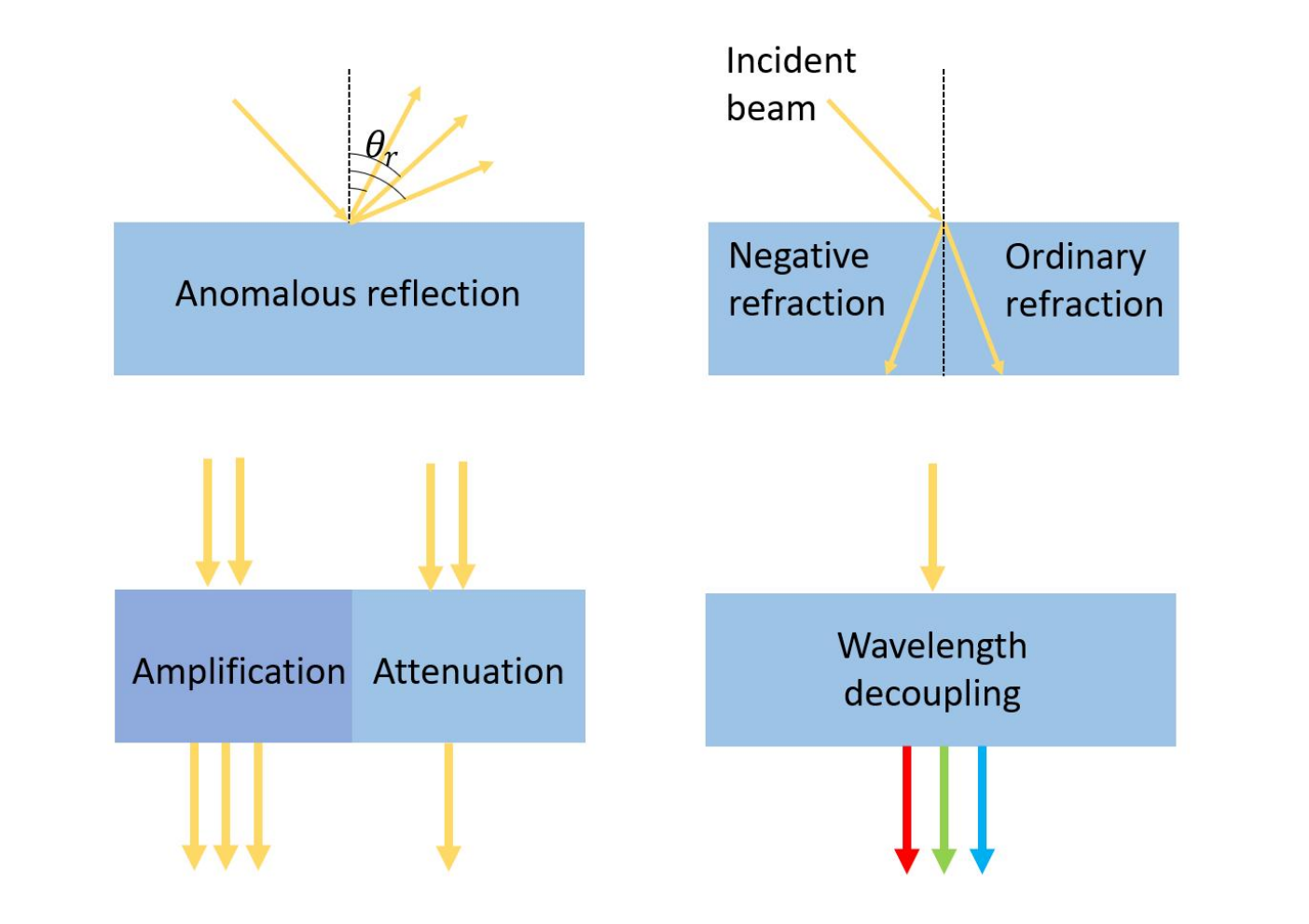
Light manipulation functionalities are illustrated in Fig. 1.2. Although the use of metasurfaces in OWC have only recently become an active area of research, their capabilities to realize light manipulation have already been tested and developed in the field of flat optics. Most of the research efforts in metasurface fabrication focus on engineering the phase profile of a wave-front since it is a critically important design feature for many applications. An example of metasurface-enabled optical phase control is the beam deflector presented in [ARX2016]. The beam deflector consists of a super-cell with fifteen nano-disks, and the diameter of each of the nano-disks can be changed to produce a phase shift from to with phase increments. The proposed design offers full -phase control and a near-unity transmission efficiency at an operating wavelength of nm. Widening the scope of metasurfaces applications requires the control of more than just the phase of the waveform. For this reason, research efforts have pushed towards achieving simultaneous control of multiple signal parameters. For example, a metasurface that can control both the amplitude and phase of light signals was proposed in [OSM2019]. The amplitude is controlled by varying the conversion efficiency of the meta-atoms, while the phase is controlled by altering the in-plane orientation of the meta-atoms. These two degrees of freedom enable complete and independent control of the amplitude and phase of the optical signal. Similarly, the work in [AHB2015] showed the possibility of achieving independent phase and polarisation control with sub-wavelength spatial resolution and an experimentally measured efficiency of up to . Another case of combining multiple functions in one metasurface is the multiplexer/de-multiplexer demonstrated in [OAM] in which wavelength, polarisation, and space multiplexing capabilities were integrated into one single ultra-thin metasurface in order to decompose the light signal into multiple channels.
The aforementioned examples demonstrate that it is possible to effectively manoeuvre the physico-chemical characteristics of metasurfaces in the visible light spectrum, which opens the door for many IRS applications in OWC systems, as will be discussed in the following sections.
1.2.2 IRS Applications in OWC
In the following, we discuss some potential applications for the integration of IRS in OWC systems.
1.2.2.1 Reflection for Blockage Mitigation
Optical signals do not penetrate through solid objects and they typically exhibit increased attenuation and less diffraction compared to RF signals. As a result, the optical link quality primarily relies on the existence of a LoS path between the transmitter and the receiver. If the LoS path is obstructed, i.e., due to the existence of a blocking entity, it is highly likely that the communication link quality will significantly deteriorate. Due to the dependency on LoS, OWC systems typically require perfect alignment between the transceiver front-ends so as to ensure a reliable transmission. Ensuring such alignment is easier in cases with no or low mobility, i.e., in VLC systems with static users. However, the case is more complicated in LiFi networks which are required to fully support high user mobility and ubiquitous connectivity. One of the key challenges in such networks is that the user terminal randomly changes its position and orientation which could lead to obstruction of the LoS link between the user and the LiFi AP.
Along with the LoS component, receivers also perceive multi-path components that result from the diffusion and reflection of light signals throughout the surrounding environment. Since both the direct LoS signal and the reflected signals carry the same data, they can be added at the receiver to maximize the total received power. In a typical indoor environment, however, NLoS signals are totally uncontrolled and nearly isotropic in their spatial distribution and are, therefore, weak at their average intensity. As a result, the effect of multi-path reflections on the received signal intensity is typically negligible [kwzz1801]. The use of IRS mounted on the walls of indoor spaces with LiFi coverage means that the reflection of the light signals could possibly be controlled so as to add significantly to the received signal at the mobile device and compensate for the loss of the LoS component in the event of a blockage. Moreover, using IRS in indoor LiFi systems can enhance the coverage of the LiFi APs by mitigating the dead-zone problem for cell-edge users. Since the coverage of an indoor LiFi AP is typically confined within the beam width of the transmitted light, non-uniform coverage distribution is typically exhibited. The reduced link reliability at the cell edge means that users moving in the proximity of the LiFi APs will need to perform frequent horizontal handovers, i.e. between neighbouring LiFi APs, or vertical handovers, between the LiFi network and the RF network. With the use of wall-mounted IRSs, users close to the wall can receive strong reflected signals that allow for meaningful signal-to-noise-ratio (SNR) [9614037]. This implies that a cell-edge user in the vicinity of the IRS can still connect to the LiFi AP despite having a weak LoS path.
The concept of using wall-mounted IRS in indoor OWC systems was investigated in [9276478]. Two types of IRSs, namely: intelligent metasurface reflectors and intelligent mirror arrays reflectors, were studied. For the metasurface reflectors, a macroscopic model for the metasurface elements is adopted to abstract them as anomalous reflective rectangular blocks. It is assumed that the phase gradient is kept constant over each metasurface element and that the phase discontinuity of each metasurface element can be tuned independently of the other elements to reflect the incident light in a specific direction, i.e., the detector’s center. For mirror array reflectors, identical rectangular mirrors with two rotational degrees of freedom are used. In the aforementioned work, it was shown that the focusing and steering capabilities of IRS are proportional to the number of reflecting elements up to a specific number of elements. Furthermore, it was shown that using a cm × cm reflector on the wall can enhance the received power by up to five times compared to the direct LoS link. The presented results imply that IRS technology provide a promising solution to compensate for LoS blockage in LiFi systems, particularly when the communication link is susceptible to blockage because of the movement of the user device or other objects. In other words, by leveraging IRS we can enable a high-performance operation for mobile devices under mobility conditions and link blockages as well as random device orientations, making LiFi resilient to these probabilistic factors.
1.2.2.2 Enhanced Optical MIMO
Multiple-input-multiple-output (MIMO) configurations are used to provide wireless communication systems with multiple transmit/receive paths so as to enable the simultaneous transmission of multiple streams of data signals. With the application of appropriate signal processing, MIMO systems can enhance spectral efficiency and received signal quality. The application of MIMO systems in OWC is an attractive solution due to the existence of large numbers of light emitting diodes (LEDs) in a single luminaire and many luminaires in various indoor settings. In the context of OWC, MIMO systems can be achieved by deploying multiple LED s on the AP side and/or multiple PD s on the user side [7314864].
While MIMO configurations have the potential to improve the performance of OWC systems, the achieved performance enhancement is highly dependant on the condition of the MIMO channel matrix. If the MIMO channel has a strong spatial correlation, the rank of the channel matrix will be low. In a multiplexing MIMO system, this means that only a few MIMO sub-channels are actually usable while the remaining sub-channels are deemed unreliable for transmitting and receiving data. In a diversity MIMO system, the high channel correlation implies that the characteristics of different diversity sub-channels are very similar. Consequently, if one of them is unreliable, the remaining sub-channels are likely to be unreliable as well, which diminishes the diversity gain. In a spatial modulation (SM) system, part of the information signal is carried on the index of the activated LED [ybth1901, yppph2001]. As a result, high channel correlation makes it hard to distinguish the difference between various spatial symbols, which results in high bit error ratios (BERs) [ybmph1701, ycphp1801]. As a result, it is clear that establishing a well-conditioned MIMO channel matrix in OWC systems is essential to ensure that various MIMO configurations can be utilized to achieve the desired advantages.
The MIMO channel conditions in OWC are different to RF. The RF wireless channels comprise multiple NLoS paths with small-scale fading, which results in MIMO channels with weak spatial correlation. On the other hand, OWC channels do not exhibit fading characteristics and rely mainly on front-end characteristics and positions. In the case of similar or symmetrical positions of multiple PD s with respect to the AP, the corresponding MIMO sub-channels will have a strong spatial correlation, which forms a major challenge in OWC MIMO systems [fh1301, pytsh1901]. One of the possible solutions to tackle the high channel correlation in optical MIMO is to carefully align the locations of the LED s and the PD s such that they create uncorrelated channel paths as was proposed in [meh1101]. While this solution could be feasible in fixed point-to-point communications, it is not always possible in LiFi systems that support high user mobility.
IRS technology provides an effective solution to improve poorly conditioned optical MIMO systems by creating controllable multi-path channels. The reflection coefficients of the IRS elements can be optimized such that the rank of the MIMO channel matrix is enhanced and the observed sub-channels are sufficiently distinguishable. The higher spatial decorrelation will enable higher spectral efficiency and boost the achievable data rate of optical MIMO systems [9614037]. The rank improvement capabilities of IRSs were studied in [oz], where a multiplexing gain was achieved even when the LoS MIMO channel is rank-deficient. It is noted that enhancing the MIMO channel rank requires joint optimisation of the reflection coefficients of the IRS elements and the transmit precoding matrix, which is a non-convex optimisation problem [9417270].
1.2.2.3 Media Based Modulation
The concept of media-based modulation (MBM) can be considered as a special case of index modulation (IM) [4382913]. While conventional IM systems employ multiple transmitters to carry distinct data symbols on the indices of the activated transmitters, MBM can be realized with a single transmitter aided with IRS. In MBM, an IRS array can be used to provide an additional dimension for data modulation by controlling the EM response of each of its reflecting elements. MBM offers some advantages compared to conventional IM including lower cost and higher flexibility [8758978, ris-mod].
The basic idea of MBM is explained in the following section. The transmission system comprises of the transmitting AP and an IRS equipped with multiple reflecting elements. Each reflecting element receives the data signal from the AP and reflects it to the intended receiver with a specific reflection coefficient. Different reflection coefficients correspond to different observed channel realisations at the receiving PD, so we can carry data bits on the state of the reflecting element. At the receiver, recovering the intended data symbols involves decoding the -ary modulated symbol as well as estimating the channel state of each IRS reflecting element. This necessitates the knowledge of the channel state information (CSI) of all the reflecting elements which could be obtained using passive pilot based channel estimation in which each IRS passively reflects the pilot sequences sent by the user to the AP to estimate its channel coefficients [9120452].
In theory, the spectral efficiency of MBM can be enhanced by increasing the number of IRS reflecting elements, as well as the number of possible reflection states. However, the enhancement is practically limited by the degree of decorrelation between the sub-channels created by different IRS elements. This is because the Euclidean distance between the MBM constellation points depends on the values of the possible channel realisations. As a result, the desired performance enhancement can be only realized if these combinations are clearly distinguishable at the receiving terminal.
1.2.2.4 Enhanced Optical NOMA
Non-orthogonal multiple access (NOMA) is a spectral efficient multi-user access technique that has been widely investigated for use in OWC systems [8713381, 7972998, 9400380]. In NOMA, signals of different users are multiplexed in the power domain by assigning distinct power levels to different users’ signals. This process is referred to as superposition coding and the power allocation coefficients are usually determined based on the users’ channel conditions. The basic principle is that users with more favourable channel conditions are allocated lower power levels than those with weaker channel conditions. Successive interference cancellation (SIC) is then performed at the receiver side to decode and subtract the signals with higher power levels first until the desired signal is extracted. NOMA has been shown to provide promising performance gain in OWC due to the high SNR and the somewhat deterministic nature of the optical channel, which facilitates the acquisition of CSI of the users with less overhead compared to RF fading channels [8352627].
The operating principle of NOMA is based on having distinct channels for different users. However, this is not always guaranteed in OWC due to the high correlation between the optical channels. In fact, the characteristics of the optical channel imply that it is likely that multiple users experience similar channel conditions, hindering the feasibility of NOMA. IRS technology offers the possibility to overcome this limitation and create distinct channels for different users by dynamically altering the perceived channel gains. Moreover, by carefully designing the reflection coefficients of the IRS elements, it is possible to create better conditions for effective power allocation which, in turn, leads to successful SIC and high reliability. Moreover, IRS-enabled NOMA offers enhanced user fairness compared to conventional NOMA systems. This is because, in conventional NOMA, the decoding order of a user depends on its channel gain value compared to the rest of the users. To this effect, users with a lower decoding order, i.e. a lower channel gain, must always decode their signals with the existence of interference from users with a higher decoding order. Dynamic IRS configuration means that it would be possible to change the users decoding order despite their locations, leading to enhanced fairness [9120476]. The work in [abumarshoud2021intelligent] proposed a framework for the joint design of the NOMA decoding order, power allocation, and the reflection coefficients in an IRS-assisted NOMA VLC system. The NP-hard multi-dimensional optimisation problem was solved by a heuristic technique with the objective of enhancing the BER performance. The presented results showed that optimized IRS leads to higher link reliability, particularly when the links are subject to the adverse effects of link blockage and random device orientation.
1.2.2.5 Enhanced PLS
The fact that light signals cannot penetrate through opaque objects makes OWC systems particularly secure in confined spaces, provided that eavesdroppers are located outside the room [PLS, 9524909, pychp2001, ycesphp2001, spkyph2101]. This means that OWC systems provide inherent physical layer security (PLS) compared to RF systems where the signals can easily be intercepted by eavesdroppers from behind a wall. Nevertheless, OWC links are susceptible to eavesdropping by malicious users that exist within the coverage area of the AP of interest.
IRS technology offers a solution to enhance the security of such systems by implementing IRS-assisted PLS techniques. Several adaptive methods can be utilized to tune the optical properties of the environment so as to enhance the link reliability for legitimate users while degrading the reception quality for potential eavesdroppers. Moreover, the IRS elements can be tuned to produce friendly jamming signals by creating randomized multi-path reflections to produce artificial noise at the eavesdropper without affecting the transmission of the legitimate user. Another possibility to use IRS to boost the PLS is to employ secure beamforming in MIMO systems. Multiple reflecting elements can be configured to produce a precoding matrix so that the signal can be decoded only at the intended receiver location to reduce the probability of signal interception.
In order to realize IRS based PLS, the secrecy performance of such systems, i.e., secrecy capacity and secrecy outage probability, must be analyzed in relation to the locations and capabilities of IRS. The work in [qian2021secure] proposed a framework for maximising the data security of an IRS-assisted VLC system. An array of wall-mounted mirrors was utilized and the orientation of each mirror was adjusted so as to maximize the achievable secrecy capacity. It was found that the IRS channel gain is highly affected by any change in the mirrors’ orientation, which makes it hard to find the optimal combination of orientation angles. In order to overcome this issue, the orientation optimisation problem was converted into a reflected spot position finding problem. As a result, the secrecy capacity can be maximized by finding the optimal position of the reflected spots for each mirror, which greatly reduces the complexity.
1.3 Case Study: High Performance IRS-Aided Indoor LiFi
1.3.1 Channel Modelling
In this section, the adopted methodology for obtaining the channel properties of an indoor LiFi network, where the system performance is enhanced via the deployment of IRSs, will be presented. Then, the effect of IRSs on the optical link budget, channel impulse response (CIR), channel frequency response (CFR) and other important channel parameters will also be detailed.
Unlike conventional RF based wireless communication systems, the operation wavelengths are in the nm region in LiFi, which makes the wavelengths comparable with atoms and molecules that comprise the surrounding materials. The penetration characteristics of the EM propagation in the visible light (VL) and IR spectra become weak due to this relative comparability. As a result, the optical channel becomes highly dependent on the surface geometry as well as the coating characteristics. In order to capture the optical channel in a realistic manner, we propose a non-sequential Monte Carlo ray-tracing (MCRT) based channel modelling technique, which is able to capture the realistic transmitter (TX), receiver (RX), environment geometry, and coating material characteristics. Note that the simplest implementation of an indoor LiFi system is to utilize off-the-shelf LEDs and PDs at the TX and RX, respectively. Thus, the information will be transmitted from the TX to RX incoherently by using the subtle changes encoded onto instantaneous light intensity, which could be detected at the RX. Consequently, the measurement of incoherent irradiance for given scenarios will be the main target in our simulations.
The proposed MCRT simulation toolbox, which is depicted in Fig. 1.3, amalgamates the geometrical non-sequential ray tracing (NSRT) capabilities of Zemax OpticStudio version 21.3.2 [zemaxopticstudio] with our custom MATLAB based computation and post-processing libraries. The accuracy of the ray-tracing in Zemax Opticstudio for only LoS and LoS-plus-NLoS cases have been reported to match the real-world measurements closely by [80211bb_2, eumhhj2001, eumhhj2002, emjhhu2101]. Accordingly, the mean squared error (MSE) between the Zemax OpticStudio simulations and real-world measurements of , and are achieved for LoS, only first-order NLoS and higher-order NLoS reflection scenarios, respectively [80211bb_2]. Therefore, a flexible and highly accurate optical channel modelling compared to the recursive method [bkklm9301, barry94] based calculations is obtained. It is important to note that the recursive method lacks the ability to model complex geometrical shapes, sources, receivers and coating materials, which is crucial in our meta-material based IRS application. As can be seen from Fig. 1.3, the environment parameters, computer-aided-design (CAD) object models, as well as source and coating material characteristics are inputted into our simulation environment. Since the main purpose of LiFi is to achieve broadband information transmission and illumination by using non-imaging off-the-shelf components simultaneously, the NSRT method is adopted in our simulations.
1.3.1.1 Generation of the Indoor Environment

A typical indoor LiFi application scenario within a cuboid-shaped room, which represents a typical indoor room structure for homes, offices, hospitals etc., with dimensions of is adopted in this work. In Fig. 1.4, the scenario under investigation is depicted, where four luminaires serve as optical APs. Each optical AP is placed at the corners of a square, with sides measuring m, that is located at the center of the ceiling. To harvest the benefits of the IRS functionality, the side walls are assumed to be covered with meta-material based wallpaper, which is depicted only for a single wall in Fig. 1.4 for the sake of simplicity. Thus, the reflection characteristics of the side walls will be altered dynamically by using IRSs to enhance the achievable SNR as well as the average error performance of a mobile user equipment (UE).
The global positions and orientations of the transmit LED array based luminaires, receive PDs and IRSs are defined by vectors, which are defined with respect to (w.r.t.) the global origin point . Note that the global origin of the system is depicted by the red dot in Fig. 1.4. The location vector of each element could be given in the format of , where , and axis components of the vector are denoted by , and , respectively. Similarly, the orientation vectors of each object are given by , where the rotation w.r.t. , and axis, in other words, within the , planes, are given by , and , respectively.
1.3.1.2 Source Characterization
The application of metasurfaces in LiFi requires the development of optical models of the transmit LEDs, receive PDs, and reflective surfaces. These models need to be as realistic as possible to capture the system performance. The accurate selection of the operation wavelengths is of the highest importance since the achievable system performance could change based on the spectral response profiles of the transmitters, receivers, and coating materials of the walls, ceiling and floor.
The generic indoor luminaires in the illumination market typically consist of a concave mirror, an LED array as the base, and a diffuser. Since our aim is to use the luminaires both for communication and illumination purposes, a LED chip array is used as the base without the mirror and diffuser structures. To take both VL and IR band characteristics into consideration, an off-the-shelf OSRAM GW QSSPA1.EM High Power White LED [gwqsspa1.em] and OSRAM SFH 4253 High Power IR LED [sfh4253] chips with a continuous radiated spectrum between the limits of m - m and m - m, respectively, are adopted in our simulations. The origin of the luminaires are assumed to be the center point of the LED array. Each LED chip within the luminaires is set to be radiating W optical power, which yields W per luminaire. The separation between each LED chip in the array is cm, and the dimensions of the luminaires are chosen to be cm. It is important to note that both the nominal wattage and dimensions of the luminaires are chosen to replicate generic commercial LED flat panel products [LEDVANCE].
The realistic radiometric spectral characteristics of the sources are defined by using the spectrum files (.spcd) in Zemax OpticStudio within our simulation environment. Thus, the related spectral distribution values for the adopted sources are obtained after processing the data-sheet values, which report the real-world measurements results. Then, the spcd files are obtained accordingly and fed into the simulation environment, which contain the relative spectral distribution coefficients w.r.t. the corresponding wavelength. The coefficients in the spcd file determine the density of a ray with the given wavelength among all the other rays with various wavelengths in MCRT. Thus, the optical power dedicated to the given wavelength will become directly proportional to the measured relative coefficients in ray-tracing simulations, which will replicate the real source spectral characteristics in the simulation environment. The relative radiometric color spectrum plots for the adopted VL and IR sources are given in Figs. 1.5(a) and 1.5(b), respectively. As can be seen from the figures, the spectrum distribution function of the white LED, , which is plotted against the wavelength, , has two peaks at and . This is primarily due to the manufacturing process of the LEDs, where a yellow color-converting phosphor coating () is superimposed onto the blue source () to achieve white light emission. The correlated colour temperature (CCT) of our adopted white LED model becomes K, which sits on the warmer side of the scale.
Similarly, the relative radiometric distribution function for the IR LED, , is also depicted against the wavelength in Fig. 1.5(b), where there is a single peak value at the . Another important parameter is the spectral spread of the adopted sources, where the bandwidth value for the IR source of shows intrinsic dominant monochromatic characteristics, where most of the power is concentrated within a relatively small range of wavelengths. On the contrary, the white source with the bandwidth value of presents a widespread poly-chromatic profile. The importance of the source chromacity for the optical link budget will be clearer in the following subsections when the coating material reflectances are presented. In our simulation environment, each source profile is represented by data points, which is the maximum value that is permitted by the simulation environment.
The realistic spatio-angular profile of the sources are also obtained from the measurement results provided by the manufacturer. The source model files with a large number of ray recordings, which are obtained by real-world goniometer measurements, are utilized to represent the adopted source spatio-angular characteristics. The main advantage of this method is the ability to model complex sources without requiring knowledge of inner opto-electrical and quantum effects dominated working principles. The radiation patterns of the VL and IR band LEDs are given by the directivity plots in Fig. 1.6(a) and 1.6(b), respectively. In these polar plots, the normalized radiant intensity distribution of the sources are plotted against the polar angle w.r.t. a source located in the direction, refer to Fig.1.4. Furthermore, the diferent colors in the plots represent the various azimuth angle scans, , , and , for the spherical coordinate system. It can be inferred from the figure that both sources have a Lambertian-like emission pattern with a strong –axis symmetry, which corresponds to the semi-angle of half power of . Compared to the ideal diffuse (Lambertian distributed) emitter model in [kb9701] with point source and receiver assumptions, the spatial domain characteristics for sources, receivers and coating materials are considered in our simulations. It is also important to determine the number of rays that will be traced in the MCRT based channel modelling approach, since it will determine the resolution of the simulations. Moreover, the statistical significance of the transmitter, receiver and reflection models needs to be maintained in MCRT by the utilization of the law of large numbers. Therefore, as a rule of thumb, the number of rays that are traced in MCRT based channel modelling applications are generally chosen to be in the order of millions [mu1501, mu2001]. To trace sufficient number of rays and realistically model the adopted sources, the spatio–angular profile of the IR band source is represented by measured rays in our simulations. For the VL band, blue and yellow spectra have been represented by measured rays each, which yields measured rays in total. In the following subsection, the optical modelling for the meta-surfaces as well as the coating materials will be detailed.
1.3.1.3 IRS & Coating Material Characterization
The coating surface characteristics for the IRS aided LiFi applications is of crucial importance since the achievable system performance will directly be affected by the total optical power that is transferred from the TX to the RX. Furthermore, the system reliability is also dictated by higher-order reflections if the direct LoS link is not available. As depicted in Fig. 1.4, the meta-material based IRSs, which are envisaged to be implanted on the wallpaper, have “ON” and “OFF” states. Please note that the “ON” and “OFF” states of the meta-materials represent two indoor application scenarios; (i) with IRS and (ii) without IRS deployment, respectively. When the IRSs are in the “ON” state, the electrical/mechanical/electro-mechanical meta-surfaces are activated and they act as micro-mirrors, which means that the reflectance of the wall increases. Since the manufacturing process of the meta-materials is complex and costly, the small grid of meta-surfaces are envisaged to be utilized on the wallpaper instead of being produced as a large single sheet of meta-surface. Therefore, depending on the density of the meta-materials, the average reflectance value of the wallpaper when the IRSs are activated could vary.
To model the IRS implanted wallpaper as realistically as possible, the relative reflectance of the side walls is assumed to be in our simulations when the IRSs are “ON”. The remaining of the incident optical power is assumed to be absorbed by the coating material of the meta-surfaces to take real-life imperfections into consideration. Furthermore, the reflection characteristics of the IRSs are chosen to follow the Phong reflection model with specular and diffuse reflection components, since the wallpaper and meta-material mixture contains both rough and shiny surface structures. Note that the diffuse reflections are scattered into rays with Lambertian distribution. In other words, the bi-directional scatter distribution function (BSDF) and the resultant intensity could be given by and , for each scattered ray, respectively. The parameter denotes the angle between the specular component and the scattered rays. In every reflection (bounce) of a light ray, of the of the incident optical power is equally divided among all the scattered rays, due to the adopted fractions of reflection and scattering coefficients. Similarly, of the of the incident optical power is allocated to the specular component. Thus, the number of the total rays in the system that must be traced after the reflection becomes , where represents the arbitrary number of reflections in the system. The parameter is the maximum number of reflections that are considered in the MCRT simulations. On the contrary, diffuse reflection characteristics with no specular components, which stem from the rough nature of the surfaces [gb7901, hjs9801, hja9802, hi0701, mu1501, mu2001], are adopted as the reflection characteristics of the wallpapers when the IRSs are “OFF”. Accordingly, the incident light rays become scattered into rays, which follow a Lambertian distribution. Lastly, the reflection profile of the wallpaper is directly dependent on the adopted surface coating material properties of the side walls.


In order to capture the realistic surface coating characteristics of the walls when the IRSs are OFF, the measurement based spectral reflectance data had to be included in our simulations. Accordingly, the wall coating material which introduces relatively low reflectance in both the VL and IR spectra, “Cobalt Green Paint Pigment”, was chosen as the main coating for the side walls as well as the ceiling. The main reason behind the selection of this material is to have a relatively small reflection contributions when IRSs are not deployed. Hence, we can simulate and report the achievable rate performance difference between IRS “OFF” and “ON” states, which correspond to the worst and best case scenarios, respectively. Furthermore, the floor of the room is assumed to be covered with a “Black Polyester Pile Carpet”, in order to mimic a realistic indoor scenario. The measured relative reflectivity weight values for the chosen materials w.r.t. the measurement spectra are obtained from the United States Geological Survey (USGS) High Resolution Spectral Library Version 7 [USGS].
The visual representations of the adopted coating materials are given in Fig. 1.7. Furthermore, the measured relative reflectivities of the adopted coating materials against the measurement spectrum, m, are depicted for data points in Fig. 1.8. In Figs. 1.9(a) and 1.9(b), the portion of the reflectivity spectrum that corresponds to the adopted source characteristics, and , is given for the chosen materials, respectively. Accordingly, the effective source spectral distribution after the multiplication of the source characteristics and the coating material reflectivity values are plotted by dotted lines under the respective source plot. It can be seen from Figs. 1.9(a) and 1.9(b) that the reflectivity characteristics of the black carpet are approximately and for the VL and IR bands, respectively. Similarly, the cobalt green paint has a relative reflectance value of and in the VL and IR bands, respectively. It is important to note that the reflectivity values of the coating material could significantly change within the spectra of each source as shown by Figs. 1.9(a) and 1.9(b). Thus, representing such fluctuations with an average value, as implemented by the recursive method based techniques [bkklm9301, barry94], would introduce a significant error in optical channel characterization. In our simulation environment, each coating material is represented by spectral data points, as this is the maximum number that is allowed by our simulation environment. In the next subsection, the receiver characterization will be detailed.
1.3.1.4 Receiver Characterization
Although other MCRT based toolkits are also proposed in the literature, the techniques in [mu1501, mu2001, mup1501] are not capable of capturing the optical channel completely since they are unable to reflect the receiver spatio-angular and spatio-spectral characteristics within their calculations. Similar to the source modelling procedure, spatial, angular, and spectral parameterization is needed for realistic detector modelling.
It is important to emphasize that two different source spectra; VL and IR band emission characteristics are adopted in this work. Therefore, the spectral responsivity curves at the RX must match the intended sources. Accordingly, two silicone PIN PDs; (i) OSRAM SFH 2716 with peak sensitivity at m and (ii) OSRAM SFH 2704 with the peak sensitivity at m are adopted as the VL and IR band receivers, respectively. Hence, non-imaging bare PD models, without any front-end optics, that are rectangular shaped with active area are generated in our simulation environment. The relative responsivity functions of the SFH 2716, , and SFH 2704, , plotted against the wavelength, , are given in Figs. 1.10(a) and 1.10(b), respectively. Accordingly, the solid blue lines depict the relative spectral response weights of each detector, where the magenta and green colors are and , respectively. Moreover, the overall spectral response for VL and IR bands, which are calculated by and , are plotted as dotted lines under the VL and IR source spectral distribution plots, respectively. As can be seen from Figs. 1.10(a) and 1.10(b) each detector closely matches their intended sources and severely attenuates the out-of-band signals. For instance, the OSRAM SFH 2716 detector responsivity curve matches the OSRAM GW QSSPA1.EM emission spactra with an average responsivity of approximately . However, the same detector filters more than of the optical power emitted from OSRAM SFH 4253. In a similar manner, the OSRAM SFH 2704 detector introduces a responsivity value of approximately for the OSRAM SFH 4253 source, where it filters more than of the optical power from the OSRAM GW QSSPA1.EM source.
The relative angular responsivity profile of the chosen detectors, which are obtained via goniometer measurements conducted and reported by the manufacturer, are fed into our simulation environment after multiple processing stages. The relative angular responsivity curves of the OSRAM SFH 2716 and OSRAM SFH 2704 detectors are given in Figs. 1.11(a) and 1.11(b), respectively. Furthermore, the ideal cosine angular profile for the receivers, , which is depicted by a dotted black line is also given as a benchmark. The parameter denotes the angle of incidence of a ray that strikes the detector. It can be seen from the angular profile of the OSRAM SFH 2716 VL band photo-detector that it closely follows the ideal cosine detection responsivity. However, this is not the case for the IR band SFH 2704 photo-detector, due to the real world geometrical imperfections introduced in the manufacturing process of the receiver micro-chips. Please note that the curves in Figs. 1.11(a) and 1.11(b) are obtained by the real world measurements. Hence, any real world imperfections and/or manufacturing errors are captured by the measurement results, unlike the ideal cosine curve. It is also important to emphasize that the non-ideal angular characteristic will play a significant role in the IR band CIRs as the received optical power values will be multiplied with a modified cosine profile of the receiver. In the next subsection, the channel models, which are obtained via MCRT simulations by considering a realistic source, IRS, coating and receiver characteristics, will be presented.
1.3.2 Obtaining the Channel Models
The multipath CIR between source and receiver could be expressed by our MCRT simulation results as follows:
| (1.1) |
where the parameters , and denote the received incoherent irradiance, total number of rays that hit the receiver and the elapsed time for the ray to reach the receiver, respectively. Note that incoming rays that strike the detector surface introduce various irradiance and time-of-flight values due to the different ray paths, even when there is no NLoS path in the system. The main reason behind this is the spatial dispersion of the rays, which emerges due to the realistic LED and PD geometrical models in our simulations. Unlike the point source and receiver assumptions in the analytical models, the source and receiver models are accurately shaped as their actual micro-chip form factor, which effects the generation and capture of the traced rays. Therefore, to reduce the temporal fluctuations caused by spatial dispersion and ensure the statistical significance, data binning also known as clustering, on is applied, which yields the discrete-time optical CIR by
| (1.2) |
Accordingly, the number of bins is calculated by
| (1.3) |
where the time of arrival for the first and last rays are denoted by and , respectively. Moreover, bin widths are also given by . The bin edge for the bin could also be calculated by . The cumulative irradiance within the given bin interval is calculated by , , if and , otherwise. Note from (1.2) and (1.3) that the temporal domain accuracy is directly related to the bin width, , where the resulting discrete-time CIR closely approximates the actual channel when the bin width approaches zero, .
Other important channel characterization parameters could also be devised by using the CIR expression obtained in (1.2). Accordingly, the optical CFR is described in terms of the discrete-time CIR as follows:
| (1.4) |
where the element-wise multiplication operation is given by . It is important to note from the above expression that the continuous time fast Fourier transform (FFT) and discrete Fourier transform (DFT) of the channel will closely approximate each other as the bin width approaches zero. The sampling frequency is calculated as . Moreover, the number of subcarriers in the DFT operation is also calculated by .
Another important parameter is the direct-current (DC) channel gain or total optical power of the impulse response, which can also be calculated by using (1.4),
| (1.5) |
The average transmitted and received optical powers could be linked by using the above DC channel gain as follows, . Similarly, by using the previous expression, the path loss (PL) in decibels could be given by
| (1.6) |
The root-mean-squared (RMS) delay spread and mean delay are two important measures to define the multipath richness of the channel, which also indicates the impact of inter-symbol interference (ISI) on the system performance. Hence, the RMS delay spread can be calculated by using the second and zeroth central moments of as follows:
| (1.7) |
where the mean delay is given in terms of the zeroth and first raw moments of by
| (1.8) |
Lastly, the relative power of the LoS component compared to the total received optical power is also an important factor to determine the dominance of the LoS path. The dominance of the LoS component directly indicates higher system reliability and link quality in cases where the direct link is broken. Accordingly, the “flatness factor” of the optical channel is calculated by using the Rician -factor as follows:
| (1.9) |
where the Rician -factor is defined as [mdcc1701]. The MCRT based channel characterization results for IRS aided LiFi will be provided for both VL and IR bands and will be presented in the following subsection.
1.3.2.1 MCRT Channel Characterization Results

| Room Dimensions | |||||
|---|---|---|---|---|---|
| LED Luminaire Positions (cm) |
| ||||
| IRS Dimensions | |||||
| IRS Positions (cm) |
| ||||
| IRS Orientations (∘) |
| ||||
| PD Positions (cm) |
| ||||
| Number of Chips per Luminaire | () | ||||
|
| ||||
| Power per Luminaire () | W | ||||
| Model of the LED Chips |
| ||||
| FWHM of the LED Chips | |||||
| Model of the PDs |
| ||||
| Effective Area of the PDs | |||||
| FWHM of the PDs |
| ||||
| Coating Materials |
| ||||
| Time Resolution (Bin Width, ) | ns |
In this subsection, the optical channels obtained with the proposed MCRT toolkit will be presented for both VL and IR bands when IRSs are ON and OFF. Moreover, the effect of user mobility on the channel parameters will also be investigated. Three mobile UE locations; L1, L2 and L3, as depicted in Fig. 1.12, are chosen to generalize the UE mobility. Accordingly, the point L1 is located near the corner and UE will receive reflections from 2 side walls. Similarly, point L2 is located near the side wall aligned with the center of the room. The UE will primarily receive reflections from a single wall. On the contrary, point L3 is located at the center of the room, which will yield a significant LoS path but negligible side wall reflections. Note that the average UE height is taken as , which is reported in [ycphp1801]. The parameter represents the average of the mean female and male height values ( cm) for England obtained in 2016 [HSE2016]. Hence, the average height of the mobile user becomes cm. The complete set of parameters used in the MCRT based optical channel simulations could be found in Table 1.1. It is important to note that the interior surfaces of the room are designed to introduce spectrum dependent reflection characteristics. When the IRSs are active, the side walls introduce mostly specular reflections, which corresponds to of all reflections Thus, of the all reflections becomes diffuse when IRSs are ON. The diffuse reflections are designed to consist of scattered rays for every surface in the simulation environment. Note that the trade-off between the time complexity and reflection accuracy in our simulations is directly controlled by the number of scattered rays, . Hence, is determined to be a sufficient value to model the reflection characteristics accurately without saturating the computational resources. The floor and ceiling always introduce diffuse reflections, similar to the side walls, when IRSs are inactive. The parameter “minimum relative ray intensity” in our MCRT simulations, which decides when to terminate the trace of a single ray is chosen to be and for VL and IR band simulations, respectively. Similar to [mu1501, mu2001], a trace of a single ray is terminated when the optical power of the light ray is decreases to and of the initial intensity in VL and IR band simulations, respectively. Note that the overall reflectivity of the coating materials in the VL band is significantly lower compared the IR band, which is compensated via smaller “minimum relative ray intensity” value. The number of rays generated per LED chip is chosen to be million in our simulation environment. Therefore, a total of million rays per luminaire are generated in IR band simulations. However, since the white LED chips consists of yellow and blue components, a total of million rays per luminaire are generated in our VL band simulations. It is also important to note that the receive PDs are assumed to capture the light rays that strike the front face of the detector surface. In our simulations, both the transmit luminaires and receive PDs are assumed to be orientated towards and axes directions, respectively. Consequently, the front face of the PDs becomes the face that looks towards direction, whereas the other face is assumed to be insensitive to the incoming light to model realistic receiver characteristics. Lastly, all four luminaires are assumed to be transmitting the same information in our channel measurement simulations without loss of generality.
1.3.2.2 VL Band Results
The CIR plots of the VL channels when the IRSs were in both the ON and OFF states are given for UE locations L1, L2 and L3 in a matrix formation in Fig. 1.13. The rows of the subplot matrix represents the location of the UE, and the columns show the states of the IRSs. Furthermore, the previously mentioned channel parameters for the same configuration are also given in Table 1.2.
For the UE location L1, the CIR results are depicted by Figs. 1.13(a) and (b). As can be seen from the figures, the magnitudes of the channel taps are significantly higher in the IRS ON state compared to when the IRS is OFF, as expected. More specifically, the peak CIR and DC channel gain in the IRS-ON state are approximately and higher compared to the IRS-OFF state for point L1, respectively. The main reason behind this significant difference is the enhanced wall reflectivity coefficients when the IRSs are activated. This effect can also be observed by the channel dispersion, where the RMS delay spread is approximately larger when IRSs are active compared to the IRS-OFF state for UE location L1. It can also be seen from the figures that the contribution of higher order reflections from the side walls, ceiling and floor surfaces yield a very high LoS spike (between ns) as well as multiple NLoS spikes (between ns) in IRS-ON case.
| IRS ON (VL Band) | |||||
|---|---|---|---|---|---|
| (ns) | (ns) | ||||
| L1 | |||||
| L2 | |||||
| L3 | |||||
| IRS OFF (VL Band) | |||||
| (ns) | (ns) | ||||
| L1 | |||||
| L2 | |||||
| L3 | |||||
The maximum number of reflections captured for the given configuration becomes when the IRSs are ON, unlike IRS-OFF case, where . Furthermore, the contribution of the NLoS channel power compared to the whole CIR is approximately and when the IRSs are ON and OFF, respectively. It is important to emphasize that this significant difference between the NLoS channels prove that the deployment of the IRSs substantially increases system reliability in cases where the direct LoS channel is blocked.
In Figs. 1.13(c) and (d), the CIR results are depicted for UE location L2. Accordingly, the peak CIR and channel DC gain when the IRSs are ON becomes lower and higher, respectively, compared to the case where IRSs are OFF. The reason behind the close match among the peak values of the CIR consists of the significantly higher LoS component that come from all four sources. Compared to location L1, the DC channel gain has increased by approximately and at point L2 when the IRSs are ON and OFF, respectively. Similarly, the time dispersion of the channel becomes higher in the case where the IRSs are ON compared to the case where the IRSs are OFF for L2. The RMS delay spread has decreased and from point L1 to L2 when IRSs are ON and OFF, respectively. The maximum number of reflections in point L2 also becomes and when the IRSs are ON and OFF, respectively. The contribution of the NLoS path compared to the whole CIR is and for the IRS-ON and IRS-OFF states, respectively. As can be seen from Fig. 1.13(c), the activation of IRSs creates the first and second tier of reflections, which are attached to the LoS component between ns. Moreover, much higher order reflections induced by the IRSs, could also be observed in between ns.
In Figs. 1.13(e) and (f), the CIR plots are provided for the mobile UE location L3. As can be clearly seen from these figures, the CIRs (especially the LoS components) are closely matching, as expected. The only difference between two cases is the larger magnitude of the higher order reflections when IRSs are active, which could be observed between ns region in both figures. However, the maximum number of reflections captured in our simulations are and for the cases IRS-ON and IRS-OFF, respectively. The reason behind this phenomena is the resolution and accuracy of our MCRT simulations, which is able to capture very small irradiance fluctuations even if they have no significance for communication purposes. The reflections captured from the side walls, ceiling and floor becomes significantly lower for location L3 even when the IRSs are active, which is due to the large physical distance between UE and the side walls. The peak value of the CIR and DC channel gain are only and higher when IRSs are ON and OFF, respectively. The channel RMS delay spread is also increased when IRSs are activated for point L3. The NLoS channel component comprises the and of the whole CIR for IRS-ON and IRS-OFF cases in location L3, respectively.
1.3.2.3 IR Band Results
The IR band CIR plots and related channel parameters are also given in Fig. 1.14 and Table 1.3, respectively.
In Figs. 1.14(a) and (b), the IR band CIRs plots for the mobile UE location L1 when the IRSs are ON and OFF, respectively, are depicted. Similar to the VL band results, the channel conditions significantly improve with the utilization of the IRSs when the mobile user is close to the highly reflective IRSs and far from the sources. As can be seen from Fig. 1.14(a), a very high peak emerged by the first and second order reflections, depicted between ns, which is merged with the LoS component. Furthermore, the third and further order reflections, depicted between ns, are also significantly enhanced with the aid of the IRSs. The peak value of the CIR and DC channel gain values increased approximately and when IRSs are activated, respectively. Similarly, an increase of in the RMS delay spread can also be observed with the employment of the IRSs compared to the case when IRSs are OFF. The number of captured bounces from the side walls, ceiling and the floor becomes and when IRS-ON and IRS-OFF, respectively. Please note that the difference between the VL and IR bands stems from the different spectral reflection profiles of the materials as well as the “minimum relative ray intensity” value in our simulations. The fraction of the NLoS component compared to the whole IR band channel becomes and for IRS-ON and IRS-OFF cases, respectively. The reason behind the higher NLoS component in the IR band compared to its VL band counterpart is the higher reflectivity values of the coating materials in the IR band (Fig. 1.8). Lastly, the maximum number of bounces considered in location L1 also becomes and for the IRS-ON and IRS-OFF cases, respectively.
| IRS ON (IR Band) | |||||
|---|---|---|---|---|---|
| (ns) | (ns) | ||||
| L1 | |||||
| L2 | |||||
| L3 | |||||
| IRS OFF (IR Band) | |||||
| (ns) | (ns) | ||||
| L1 | |||||
| L2 | |||||
| L3 | |||||
The IR band channel impulse response plots and the related parameters are also provided for UE location L2 in Figs. 1.14(c)-(d) and Table 1.3, respectively. Similar to the VL band results, the impact of the IRSs could be seen from Fig. 1.14(c) in the first and second order reflections ( ns) as well as the higher order reflections ( ns). However, the effect of the IRSs are not as dominant as in location L1 due to the dominant LoS link ( order reflection). The peak value of CIR and DC channel gain when IRS-ON are lower and higher compared to IRS-OFF case, respectively. Again, the reason behind this is the effect of the IRSs on the higher order reflections, which also indicate that the system capacity will be higher when IRSs are activated if the direct LoS link is blocked. The RMS delay spread also increases around when the IRSs are activated, which shows the significance of the higher order reflections. Compared to location L1, the DC channel gain increases by , whereas the RMS delay spread decreases by compared to L2 when the IRS-ON, respectively. For cases where the IRSs are OFF, the DC channel gain increase is approximately and the RMS delay spread decrease is around from point L1 to L2, respectively. Moreover, only the NLoS path contributions compared to the whole channel becomes and for IRS-ON and IRS-OFF cases, respectively, when the UE is located at L2. The number of bounces encountered in our MCRT simulations becomes and for IRS-ON and IRS-OFF cases, respectively, when the UE is at L2.
In Figs. 1.14(e) and (f), the CIR plots for mobile UE location L3 when IRSs are ON and OFF, respectively, are depicted. The peak value of the CIR and DC channel gain are increased and when the IRSs are activated for UE location L3, respectively. As can be seen from the channel parameters as well as Figs. 1.14(e) and (f), the effect of the IRSs on the main lobe, between ns, is minimal due to the dominant LoS power. However, the optical power emerges due to the higher order reflections, between ns, is significantly higher in IRS-ON case compared to IRS-OFF. Furthermore, the RMS delay spread of the channel increases by more than when the IRSs are activated at location L3. The maximum number of bounces captured in our simulations for the case when the IRSs are ON and OFF becomes and , respectively, when the UE is at L3. The NLoS contribution against the whole channel optical power also increased from to when the IRSs are activated for a mobile user located at L3.
1.3.3 The Achievable Rates for IRS-aided LiFi
In this subsection, the achievable rate curves for the IRS-aided indoor LiFi application scenario will be provided. The maximum achievable system capacity for LiFi systems could simply be calculated as follows [kb9701, hycvppai2001]:
| (1.10) |
where the average transmitted optical power, DC channel gain, the effective noise power in the electrical domain and communication network’s effective bandwidth are denoted by , , and , respectively. Note that the effective noise term at the UE consists of the addition of shot and thermal noises, where the shot noise emerges as a result of ambient light sources and the information bearing signal itself. In cases where high ambient light power at the PD is significantly larger than the transmit signal power, the shot noise becomes signal independent. Therefore, the high intensity shot noise at the RX could be modelled as a summation of independent low power Poisson processes, which could be approximated as a zero mean Gaussian distribution. Consequently, the effective noise could be modelled as additive white Gaussian noise (AWGN), , where . A real Gaussian distribution with mean and variance is denoted by .
By using Tables 1.2 and 1.3, the DC channel gain values for both the VL and IR band could be obtained for the cases where IRSs are ON and OFF w.r.t. UE locations L1, L2 and L3. Also note from Table 1.1, the transmitted optical power is chosen to be W per luminaire. The effective channel bandwidth, , for the considered system could be calculated by using the expression,
| (1.11) |
Please note from (1.10) and (1.11) that typical LiFi networks are not limited by channel bandwidth, but by the the electrical domain bandwidth of the front-end opto-electronic devices such as LEDs and PDs. In this work, the optical channel bandwidth is considered as the main limiting factor for the system as it inherently emerges. On the contrary, the electrical channel bandwidth, caused by the font-end opto-electronic frequency response, is strictly dependent on the manufacturing technology behind the transmit LEDs and PDs. Therefore, the channel impairments introduced by the electrical domain components could be avoided as technology advances. Moreover, in our simulations, the number of DFT subcarriers and the effective optical channel bandwidth could be calculated by using the values in Table 1.1 as and GHz.
In Figs. 1.15, the achievable capacity plots for IRS-ON and IRS-OFF cases when the UE is located at L1, L2 and L3. Accordingly, the VL band plots are given for the dB SNR-per-bit () region in Fig. 1.15(a). As can be seen from figure that the maximum achievable capacity increases exponentially within the low SNR region. Please note from Figs. 1.13 and 1.14 that the channel magnitudes are in the and region, thus, the electrical domain path loss at the RX becomes about and dB, respectively [phd_Fath]. Therefore, the SNR measured at the TX side within the interval of dB will be classified as the low SNR regime for this application. For UE location L1, the achievable data rate becomes approximately and Mbits/sec when the IRSs are ON and OFF, respectively. Similarly, for L2, the achievable rates of approximately and Mbit/sec for cases where the IRSs are ON and OFF, respectively. Lastly, approximately and Gbit/sec data rates are achieved for the UE location L3 when the IRSs are active and inactive, respectively.
The IR band achievable capacity plots for IRS-ON and IRS-OFF cases when the UE is located at points L1, L2 and L3 are depicted in Fig. 1.15(b). It is important to note that the overall capacity values are higher in the IR band compared to the VL band results due to the higher reflectivity profiles of the coating materials in the IR spectra. For UE location L1, the capacity rates of approximately Gbits/sec and Mbits/sec are achieved when IRSs are ON and OFF, respectively. Moreover, the achievable rates become approximately Gbits/sec and Mbits/sec for IRS active and inactive cases, when the UE is located at L2. Finally, for UE location L3, the achievable rate of and Gbits/sec are obtained for the IRS-ON and IRS-OFF cases, respectively. Please note that based on both VL and IR band plots, the maximum capacity values are achieved for each UE location when the IRSs are activated.
1.4 Challenges & Research Directions
The concept of IRS provides opportunities for achieving unprecedented capabilities when it comes to signal and link manipulation. However, realising such capabilities is subject to overcoming the challenges associated with the realisation of this concept. In this section, we highlight some of the challenges and open research directions related to the integration of IRS in OWC systems and propose a road map for future research directions.
1.4.1 Modelling and Characterisation
One of the challenges in the research and implementation of the concept of smart walls in OWC systems is the development of realistic and accurate channel models. More specifically, there is a need to establish realistic models that take into account the type, capabilities, and limitations of different possible IRS structures in order to capture the fundamental behaviour and performance limits of such systems. Moreover, since classical optical channel gain models might not be suitable, it is critical to understand the CIR of different metasurfaces over the range of optical wavelengths. In particular, there is a need to quantify the efficiency and response time for achieving specific functionalities such as amplification factors, absorption capabilities, anomalous reflection, etc. Additionally, it is critical to understand how such systems perform in different mediums such as underwater and outdoor environments with high ambient noise.
1.4.2 Inter-symbol Interference (ISI)
It has been reported in the previous section that the deployment of the IRSs in typical indoor LiFi networks increases the achievable data rate values significantly both for VL and IR spectra. However, one of the biggest challenges for IRS-aided LiFi arises from the inflated channel time dispersion. The increase in the channel delay spread values could effectively reduce the system performance due to the increased ISI. The ISI could be avoided in multi-carrier transmission methods, especially in orthogonal frequency division multiplexing (OFDM), by the utilization of the cyclic prefix (CP). Furthermore, with the activation of the IRSs, the channel frequency selectivity will also increase which means that the SNR in each subcarrier will significantly differ from each other. Consequently, in order to avoid further channel impairments which could emerge with the utilization of IRSs, suitable CP length selection as well as adaptive bit loading in OFDM are required. A detailed investigation of the optical OFDM systems and their error performances under the frequency selective channel that emerges in IRS-aided LiFi is necessary to obtain better insights on the performance of such systems.
1.4.3 Channel Estimation
The availability of accurate CSI for all the channel paths created by massive numbers of tunable sub-wavelength reflecting elements proves to be a challenging task. Traditional CSI estimation techniques might be unpractical for real-time estimations given the high dimensions of the channel vectors for each network user, particularly if higher order reflections are considered. There is a need to quantify the trade-off between distributed and centralized CSI acquisition approaches and to come up with intelligent and cost-effective methodologies. Distributed CSI acquisition approaches employ local estimation at each IRS array which requires sensing and processing capabilities. Centralized CSI acquisition approaches, on the other hand, employ a central control unit, typically at the AP. The central unit is responsible for performing the CSI estimation for all network entities, which are then utilized for optimisation and reconfiguration decisions that are executed centrally. The obvious advantage of the centralized approach is that the IRS is not required to perform exhaustive sensing and processing, leading to lower energy consumption and a simpler hardware design. The main challenge of this approach is the signalling overhead, which occurs between the central unit and the IRS.
1.4.4 Real-time Operation
Integrating IRS arrays with a high number of reflecting elements and varying functionalities inevitably results in high operational complexity which entails increased computational, energy, and overhead cost. The IRS elements need to be reconfigured in real-time to provide precise control over their optical functionalities, which is decided based on the varying system conditions. Such an operation is not trivial and entails different trade-offs. For example, there is a need to develop activation strategies that take into account different metrics, such as throughput and fairness, in order to balance the desired performance enhancement and the associated energy consumption and time delay. Also, how often the reflecting element must be reconfigured must be determined i.e., whether this should be performed with each channel realisation or when a change occurs in the user location. Incorporating data-driven optimisation tools such as deep learning, reinforcement learning, and federated learning could provide viable solutions to achieve time-efficient optimisation.
References
- [1]